The formation and use of hierarchical cognitive maps in the brain: A neural network model

ABSTRACT

Many researchers have tried to model how environmental knowledge is learned by the brain and used in the form of cognitive maps. However, previous work was limited in various important ways: there was little consensus on how these cognitive maps were formed and represented, the planning mechanism was inherently limited to performing relatively simple tasks, and there was little consideration of how these mechanisms would scale up. This paper makes several significant advances. Firstly, the planning mechanism used by the majority of previous work propagates a decaying signal through the network to create a gradient that points towards the goal. However, this decaying signal limited the scale and complexity of tasks that can be solved in this manner. Here we propose several ways in which a network can can self-organize a novel planning mechanism that does not require decaying activity. We also extend this model with a hierarchical planning mechanism: a layer of cells that identify frequently-used sequences of actions and reuse them to significantly increase the efficiency of planning. We speculate that our results may explain the apparent ability of humans and animals to perform model-based planning on both small and large scales without a noticeable loss of efficiency.

KEYWORDS:

• Neural Network models
• motor control
• model-based behaviour
• neural development
• self-organization
• population coding

Introduction

Statement of research question

How might a biologically plausible neural network based on the architecture and operational principles of the brain learn to perform hierarchical model-based action selection as it explores a sensory environment?

Broad rationale for research question

The experiments of Tolman (Tolman 1938, 1948; Tolman et al. 1946) suggested that rats attain an internal model of their environment, called a cognitive map. Furthermore, they suggested that this cognitive map was necessary to respond quickly to changes in the reward available in an environment or to changes in the structure of the environment.¹ Examples of these are latent learning tasks and detour tasks, described more fully in Section 1.3.

Extensive modelling efforts (Dolan and Dayan 2013) have validated this claim. Despite the development of sophisticated “model-free” algorithms it has thus far been impossible to replicate certain observed behaviours without using a cognitive map representation (Russek et al. 2016; Fakhari et al. 2018).

Several neural network models have studied the formation and use of cognitive maps.² However, many of the major questions around map-based planning have not yet been fully answered. How are spatial and non-spatial cognitive maps formed, stored, retrieved and used at the neural level? Furthermore, how are these processes affected by scale? It is uncertain how the storage and usage of cognitive maps differs between the small-scale mazes used in rat-based experiments and the large-scale maps of, say, a town, that a human would use to navigate. These problems are considered in Sections 3 and 5.

There is some evidence that map-based planning can take place on very short timescales but also on much longer timescales, frequently abstracted from much detail about individual muscle movements (Botvinick et al. 2009; Ramkumar et al. 2016). Behavioural research is currently investigating such “high-level” or “hierarchical” environment representations and map-based planning, and the results of these investigations are detailed in Sec. 1.5. Furthermore, a considerable amount of work in artificial intelligence research has been dedicated to investigating different forms of hierarchical planning in the context of Markov Decision Processes (MDPs) and Reinforcement Learning (RL); this research is discussed further in Sec. 1.6.

We believe that by modelling hierarchical, map-based planning in a biologically plausible neural network architecture – one which relies on local Hebbian learning to model synaptic plasticity and which self-organizes its connectivity from sensory and motor inputs as the simulated agent explores its environment – we can begin to produce predictions of the neural and behavioural correlates that might accompany this form of planning. In particular, to produce predictions about how an unsupervised neural architecture could learn to represent useful sections of previously experienced trajectories and use these to plan at larger scales with greater efficiency, yet still in a biologically plausible fashion. Furthermore, by investigating the constraints of such a model, we can predict the features that a planning model needs to have in order to begin planning hierarchically, therefore constraining the space of possible action selection models.

Neurological investigation of cognitive maps

Although Tolman’s experiments were not conclusive, the cognitive map hypothesis has been greatly strengthened by further experimental evidence since it was originally proposed. In particular, the discovery of place cells in the hippocampus (O’Keefe and Nadel 1978) gave a neural substrate in which the cognitive map might be stored. The later discovery of grid cells in the entorhinal cortex (Hafting et al. 2005) gave rise to theories that combinations of grid cell inputs might give rise to place cell responses (Rolls et al. 2006; McNaughton et al. 2006) and so about how the cognitive map might arise. A little later still, the work of Johnson and Redish 2007 (Johnson and Redish 2007) showed apparent neural correlates of map-based planning in place cells: rats at a choice point sent waves of activity along the place cells that represented various future paths, apparently selecting between them in a process dubbed “mental time-travel”.³

Several experiments have provided indications that cognitive maps also exist for non-spatial domains. In particular, Kurth-Nelson et al. (Kurth-Nelson et al. 2016) analysed whole-brain magneto-encephalographic (MEG) data while subjects performed a non-spatial navigation task⁴ and found that (a) the current state could be reliably decoded from MEG data and that (b) once the task had been learned, spontaneous MEG activity encoded legal paths through the environment. These paths appeared as reverse sequences of up to four states.

An experiment by Aronov et al (Aronov et al. 2017) has also shown the existence of “place cell” representations for non-spatial state-spaces. Mice were given the ability to alter auditory stimuli along a continuous frequency axis and cells developed in the hippocampal CA1 and the medial entorhinal cortex that have discrete firing fields along particular areas of the frequency axis. These cells overlapped with spatial place cells and grid cells but not in any organized fashion, which suggested that some spatial cells were being randomly repurposed for this new representation. Interestingly, these neurons appeared to be task-selective; when Aronov et. al. presented the same mice with the same stimuli (sweeps of the same frequency and duration) outside the context of the task, they found very little activity in the cells that had earlier fired reliably at different parts of the same axis.

Algorithms for stimulus-response and cognitive-map based planning

Historically, two kinds of animal behaviour tasks have been presented as arguments against purely model-free theories of planning in the brain: revaluation tasks, which examine whether animals adjust their behaviour appropriately following changes in the reward function, and contingency change tasks, which examine whether animals change their behaviour appropriately following changes in the transition structure of the environment (for example, a blocked or opened passageway in a maze) (Tolman 1948; Russek et al. 2016). Model-free reinforcement learners perform poorly in these tasks because they cache the cumulative expected rewards that they expect from different state-action combinations and – without a transition model of the environment – have no way of updating these cached values post-manipulation except to relearn its Q-function. In comparison, model-based reinforcement learners can immediately update their value-functions and policies, continuing to produce adaptive behaviour in the face of environmental changes or altered rewards (Russek et al. 2016). Russek et al. 2016 found that a model-free approach, even augmented with a successor representation (Russek et al. 2016), could not solve contingency change tasks. These tasks, in particular a variant of the Tolman detour task described later in this paper, required an explicitly model-based reinforcement learning approach.

The role of hierarchical representations in planning behaviour

An important objective of this paper is to investigate the production and use of hierarchical map elements in a biologically plausible neural network model. Accordingly, this section will discuss the nature of these hierarchical elements in vivo as far as it can be deduced from behavioural studies.

Extensive evidence shows that humans represent space in a regional and hierarchical fashion. The regional representation of spaces affects the ability of participants to judge the spatial relationship between locations in different regions (Hirtle and Jonides 1985) and their behaviour when searching for a specified location (Hölscher et al. 2008). Regional effects seem to occur even in spaces whose hierarchical structure is not explicitly defined (Hirtle and Jonides 1985).

Experimental work has also indicated that humans plan routes at different levels of the hierarchical representation. When giving route directions, either in advance or during travel, participants reliably produce high-level route segments in order to optimize information-to-memory-load (Klippel et al. 2003). Furthermore, participants reference elements of a city in order from the most general to highly specific local references (Tomko et al. 2008), signifying that most people store hierarchical spatial information in the same way and are able to predict what level of information other people are likely to recognize. Timpf et. al. (2003) break down highway navigation into three levels of abstraction: route planning operates on a very high level, finding routes given certain constraints; driving is performed at a fine level; and people produce driving instructions at a level partway between the two, dividing the route into segments that amalgamate a certain amount of driving activity (Timpf and Kuhn 2003). Wiener & Mallot (2003) similarly show that humans appear to use a fine-to-coarse planning heuristic when navigating: a route plan contains fine-space information for the close surroundings and coarse space information for the rest of the route (Wiener and Mallot 2003). There is also evidence that route familiarity is an important element in human navigation (Payyanadan 2018).

We believe that the scale on which high-level route segments are generated and used depends on the size of the task in question. People give directions of a roughly similar length for routes whose lengths differ by orders of magnitude, provided that route fragments of the appropriate scale exist, indicating that the existence of high-level actions (driving instructions) allows complex routes to be compressed into a practical length. At the same time, planning tasks performed at the same level of abstraction show planning times are partially proportional to absolute path length (Howard et al. 2014).

We believe that a model of map-based planning should explain both the generation of high-level path fragments as well as how planning operates at any given level of abstraction.

Hierarchical representations in markov decision processes

If we consider MDP solving – and behavioural planning more generally – as the process of searching for a nearly optimal solution to a problem in a very large space of potential actions, it becomes clear that as that space grows, the process of searching for a solution becomes more difficult, until the problem becomes computationally intractable for a naive planner.

For an algorithm to successfully obtain its goals within a very large state space, it must either find a way to shrink that space or to search through that space more efficiently. An example of the former is the set of algorithms that try to abstract away irrelevant state attributes to describe the task in the minimum number of states (Ebitz et al. 2018). An example of the latter is the option framework, defined by Sutton and Barto in their 1999 paper “Between MDPs and semi-MDPs: A framework for temporal abstraction in reinforcement learning” (Sutton et al. 1999). The original formulation of the option framework speeds up the planning process in an MDP through the provision of Options, little chunks of policy that can be predefined by the coder or learned/imported from previous tasks. Each option consists of an initiation set (states where the option may be used), a termination set (states where the option ends and the agent starts choosing actions normally again) and a policy (a set of state-action combinations that moves the agent towards a state in the termination set). Hierarchical Reinforcement Learning, as seen in Botvinick 2009 (Botvinick et al. 2009), implements options in order to allow the agent to explore the environment in a faster and more rewarding fashion.

Options can be specified by modellers, as in Botvinick 2009, but ideally an agent using the option framework should be able to discover useful options on its own. The two main approaches can be summed up as sub-goal based or policy based.⁵ Subgoal-based option discovery uses various techniques to identify useful states as subgoals. These states are usually either bottlenecks – states that connect together two otherwise-isolated sets of states – or frequently visited states. Having identified these subgoals, a secondary reinforcement learning process is used to create a policy for reaching those subgoals, rewarding the agent with a pseudo-reward when it reaches those subgoals (Botvinick et al. 2009; Taghizadeh and Beigy 2013; Kulkarni et al. 2016; Tessler et al. 2016; Vezhnevets et al. 2017).

While subgoal-based option discovery focuses on the termination of an option, identifying a useful sub-goal and then learning an option policy that can lead the agent to that subgoal, policy-based option discovery ignores subgoals and tries to identify useful sub-policies directly. One common approach is to search many solutions for common policy elements (Pickett and Barto 2002; Girgin et al. 2010). Florensa et al. (Florensa et al. 2017) have produced a hierarchical deep reinforcement learner along policy-based lines by producing a framework for learning skills and applying them in different tasks. Their framework consists of an unsupervised procedure to learn a repertoire of skills using proxy rewards, as well as a hierarchical structure for reusing those skills in future tasks. Skills appear to be represented as policies, similar to other approaches in this subsection.

Literature review

Representing an environment within a cognitive map

There are various ways for a cognitive map to encodes the topology of an environment. One potential representation is the use of state (place) cells. These place cells are connected together by recurrent synaptic connectivity in such a way that each state is connected to its neighbouring states. This is probably the most simple form of cognitive map, and Matsumoto 2011 (Matsumoto et al. 2011) shows that it is possible to use this map to plan (using a mechanism described below). However, this form of map does not encode any information on the actions that are required to move the agent from one state to another. Planning in this context can therefore only mean assigning value to different states, marking some as more desirable and some as less desirable. This form of cognitive map therefore implicitly predicts that some other, unmodelled, mechanism must exist that knows how to move the agent from one state to another. In other words, this form of cognitive map does not reproduce an extremely important part of the planning mechanism.

Another form of cognitive map, used by Friedrich 2016 (Friedrich and Lengyel 2016), is based on state-action cells. These cells encode a combination of a particular state with a particular action taken in that state. They are connected together with recurrent synaptic connectivity that encodes a causal relationship. If a cell encodes a state-action combination that produces a transition to a particular successor state, that cell will be synaptically connected to other cells encoding the successor state. This means that a state-action map can encode not only how different states are connected but also what actions an agent should take to move between these states.

A variation on the state-action map is the transition map used by Cuperlier 2007 (Cuperlier et al. 2007), which uses several different kinds of transition cells to encode the cognitive map. Some of these cells encode a unique transition between two states, without encoding the action that produces that transition, and these cells effectively work in the same way as state cells. Other cells encode a combination of a given transition and a motor action that produces that transition and so end up resembling state-action cells. A problem with this form of map representation is that it does not seem likely to generalize well to nondeterministic environments. In certain environments, a single state-action combination may produce many state transitions. In a state-action model, these transitions may all be represented using recurrent synaptic weights. By contrast, in a transition cell model each transition requires its own cell. As the ratio of transitions to state-action combinations increases, the ratio of required transition cells to required state-action cells increases.

More complex cognitive maps (Hasselmo 2005, Martinet 2011 (Hasselmo 2005; Martinet et al. 2011)) still fundamentally use a state-action encoding for the cognitive map but incorporate these cells within complex minicolumn structures designed to facilitate various elements of the planning process. Functionally, minicolumns allow for much more detailed circuitry to be easily modelled and iterated across the cognitive map representation. This makes minicolumn models more powerful than models using other representations but also more complex and less clear.

The form of an agent’s cognitive map will inevitably affect the mechanisms that are required to plan using this map. From this perspective, the most important distinction between the various forms of maps is between those maps that incorporate actions implicitly (a pure state cell map) and those that incorporate actions explicitly within the cognitive map (all others). A pure state cell map inherently predicts that planning takes place at the state level, and that some other mechanism exists which encodes the causal knowledge of how to move from one state to another and that outputs actions to do so. In other words, a pure state model predicts that planning and acting are two fundamentally separate processes, which output a set of desired transitions and a set of actions respectively. By contrast, a state-action representation predicts that these two processes are inherently interlinked. This claim could be explored experimentally by looking for cases (if they exist) where people appear to be able to plan a solution to a problem (i.e. to give a set of transitions between states) but are not able to give a set of actions which would perform those transitions. This would demonstrate that it is possible to disrupt the action-production process without disrupting the planning process. The existence or non-existence of such cases might support a state-based or state-action based account.

Another open question is how these representations should scale. Of the models cited, all of them except for Matsumoto 2011 and Friedrich 2016 are discrete: they assume that states and actions are separable from one another. This has two consequences. The first is that in many cases the associated cognitive maps encode an artificial separation between different states and different actions. Either they are described purely in the context of tasks with discrete state spaces (such as the grid word tasks used throughout this paper, where you are either in one grid square or another grid square), or the models designate certain points in a continuous state space as “states” and ignores all of the points in between. The same is true of actions, where a limited set of discrete actions is made available for the agent to choose between. The second consequence of using a discrete state space – at least in the reviewed models – is that they do not handle scaling well. As the size of the environment increases, either the number of discrete states must increase or the ability of the map to encode the state space must decrease. For this reason, the models reviewed in Sec. 2 all have small state spaces.

The alternative is a continuous representation, where each input neuron represents some form of function in the joint space of states and/or actions (e.g. a place cell with a gaussian receptive field). In this case states and/or actions can be represented as a unique combination of distributed input neuron firing. Two models deal with such continuous representations: Matsumoto 2011 and Friedrich 2016 (Martinet et al. 2011; Friedrich and Lengyel 2016), but these models are also the most limited in terms of explaining the mechanisms around the formation and use of these maps: Matsumoto 2011 does not address the encoding of causal relationships between states, Friedrich does not address the formation of the cognitive map, and neither of them model the process of reading out the results of the planning process using neural mechanisms. It seems likely that the complexity of modelling continuous representations is responsible for the more limited scope of these models.

Encoding of the cognitive map in recurrent connectivity

All of the reviewed networks encode the cognitive map as a set of synapses that connect the cellular substrate (state/place cell, state-action cells or neocortical minicolumns). These synapses can be assigned algorithmically or they can be self-organized using a variety of methods.

In Cuperlier 2007, Martinet 2011 and Friedrich 2016 (Cuperlier et al. 2007; Martinet et al. 2011; Friedrich and Lengyel 2016), the connectivity is not self-organized using biological processes. Instead, as the agent explores its environment, the appropriate cells are connected together algorithmically. In the case of Cuperlier 2007 (Cuperlier et al. 2007), which uses transition cells (see above) this means setting the synapses between the current and previous transition cell to an arbitrary positive value after a state transition. In Martinet 2011 and Friedrich 2016 (Friedrich and Lengyel 2016), it means doing the same with state-action cells.

Erdem & Hasselmo 2012 (Erdem and Hasselmo 2012) model a mechanism which is slightly more consistent with the known neurobiology. In this model, the topology cells (which represent the topology of the environment) are essentially place cells, but are connected together using a learning rule which does not incorporate any firing information related to the topology cells that are being connected together. Instead, the equation used implicitly combines activation, competition and recency cell activity to connect topology cells together as a function of a “recency signal”. This implicit modelling seems to presuppose that recency cell activity would activate the appropriate topology cells in certain ways, that certain forms of competition could be applied to the topology cells such that their firing came to encode the desired function of their inputs, and that Hebbian learning could then connect the still-firing topology cells together in such a way as to obtain the desired connectivity. Essentially, the learning rule implicitly describes an extended sequence of mechanisms that are not explicitly modelled. Since these mechanisms are not explicitly simulated it cannot be assumed without reservation that they would operate as hypothesized and without unforeseen side-effects. The possibility that – if these mechanisms were implemented explicitly – Erdem & Hasselmo 2012 might be unable to learn a cognitive map is a limitation in this work.

Hasselmo 2005 (Hasselmo 2005) uses a Hebbian local learning rule that implements a “memory buffer” which holds activity from the input state, thus allowing self-organization of the synapses between the minicolumns that encode the cognitive map. The actual self-organization is highly complex but appears to be Hebbian.

Finally, Matsumoto 2011 (Matsumoto et al. 2011), which encodes the cognitive map between place cells with large, overlapping fields, is able to encode the relationship between states using a simple Hebbian rule. Each location in the state space is signified by the combined activation of multiple state cells. As the agent moves through the environment, it will move from one receptive field to another, and as it moves between the two receptive fields both place cells will be firing simultaneously. A simple Hebbian learning rule is therefore able to connect neighbouring place cells.

Planning mechanisms

Most current models of biologically plausible cognitive map-based planning (Cuperlier et al. 2007; Martinet et al. 2011; Friedrich and Lengyel 2016) are based on the principle of propagating activity from a goal representation through the synaptically encoded cognitive map.

The basic paradigm is that of propagation with decaying activation. In this paradigm, the cells encoding the cognitive map are stimulated at one location, or several locations, encoding the goal state that the agent is required to navigate to using its cognitive map. This activity propagates through the cells encoding the cognitive map, such that cells close to the goal receive high activity and fire at a high rate, while cells further from the goal receive much less activity and fire at a much lower rate. In effect, a gradient of activity is created with the cells that represent the goal state(s) having the highest firing rate and the state cells or state-action cells that are far away in the map (separated by many transitions) having very low or no firing.

If the map is made up of state cells, as in (Matsumoto et al. 2011), this gradient effectively encodes a value-function: states represented by high-firing cells are highly valuable, states represented by low-firing cells are not valuable.

If the map is made up of state-action cells, as in (Friedrich and Lengyel 2016), this gradient effectively encodes a Q-function: state-action combinations represented by high-firing cells are valuable, state-action combinations represented by low-firing cells are not so valuable.

The decaying-activation paradigm allows successful planning. In particular, Martinet 2011 show that a decaying-activation model is able to reproduce the characteristic behaviour of rats performing a Tolman detour task (Martinet et al. 2011; Alvernhe et al. 2011). It also reproduces the latent learning phenomenon, in which rats which have previously been allowed to explore a maze in the absence of explicit external reward are able to successfully navigate to a reward in that maze much faster than rats which lack this experience (Tolman 1948). Various refinements and extensions have been proposed that allow decaying-activation models to memorize the path to previous goals (Matsumoto et al. 2011), take shortcuts (Erdem and Hasselmo 2012) and store environmental maps at different resolutions (Martinet et al. 2011). However, although these extensions can produce interesting effects under certain conditions, they tend to compromise either the biological plausibility of the model or its robustness. For example, the linear probe mechanism proposed by Erdem & Hasselmo 2012 (Erdem and Hasselmo 2012) allows agents to take shortcuts through unexplored space but compromises the model’s ability to navigate around obstacles.

Although a decaying-activation planner can reproduce basic planning behaviour, as well as replicate seminal tasks such as the Tolman detour task, the behaviour of a decaying-activation planner does not appear to match experimental observations in certain ways. The first and most important of these is that if the goal is sufficiently distant, and a sufficiently large number of actions are required to reach it, then the decaying activity will decay to zero before it reaches the agent’s current state. Since it is (the gradient of) this activity that defines either a value function or a q-function for each state, if no activity reaches a state or set of states then the agent has no value information available about those states. The agent will therefore not be able to produce a useful action. A decaying-activation planner will therefore fail to produce appropriate actions if the distance to the goal is too great. This does not seem to be consistent with evidence that animals can plan and navigate in large-scale environments (Geva-Sagiv et al. 2015).

A second issue with planning using decaying activation is that it may be vulnerable to noise. If the gradient of decaying activity spreads over a large number of states, then the relative firing rates of cells representing different states (or different actions within the same state) are likely to be similar. The firing rates of these cells are used to indicate the relative values of the associated states or state-actions; if they are very similar then small changes due to noise may make a big difference to their relative values and cause very different actions to be selected. A decaying-activation mechanism may take a relatively long time to output actions. Cuperlier 2007 (Cuperlier et al. 2007) reads out an action only when the activity in the network is considered “stable”, which presumably requires either a set period of stabilization or a mechanism that judges the stability of the activity dynamics. Hasselmo 2005 waits for a specific period of time before reading out an action and thereby risks reading out too early (before activity has reached the right part of the map) or too late (when the situation has changed or time has been wasted).

Hierarchical behaviour

In general, current models of biologically plausible map-based planning do not consider how cognitive map representations and map-based planning should scale. As observed above, these models use a decaying-activation mechanism and so are unlikely to produce appropriate scaling because the activity is likely to decay too much in larger maps. To our knowledge, the only exception at present is work by Martinet 2011 (Martinet et al. 2011), which introduces an extra map at a lower resolution. This mechanism uses proprioceptive feedback to merge states that are considered to be functional aliases of each other, extending the range over which their model can plan before the decaying activation disappears completely. This could potentially explain the relationship between planning time and distance described above. In this paper, we propose an alternative explanation: that over time, useful sequences of small-scale state-action combinations are encoded as functional behaviours or skills, allowing an agent to produce faster but more stereotyped behaviour at larger spatial scales.

A hardwired model for producing hierarchical behaviour using sequence cells

Hypotheses

We hypothesize that the hierarchical route representations observed experimentally (Klippel et al. 2003; Timpf and Kuhn 2003; Wiener and Mallot 2003) could be produced by using behaviourally significant sequences of state-action combinations to represent certain elements of the route more concisely and abstractly. We further hypothesize that these sequences could subsequently be implemented during planning as “mental shortcuts”. In this case, the agent would be able to plan partially at a more abstract level; it would select sequences rather than individual state-action combinations. By representing a long route as 3 sequences rather than 500 individual state-action combinations, the agent would greatly reduce the number of choices required to plan that route. In effect, these sequences would function as high-level actions or blocks of policy that move the agent from one state to a far-off state, allowing the agent to plan across large sections of the state-action space concisely and efficiently.

This section will discuss how these sequences can be encoded within the network and how they can be used to plan faster and more efficiently. As such, this section will not discuss the process responsible for learning sequence representations. Section 5 is dedicated to the process of learning these sequences.

Model overview

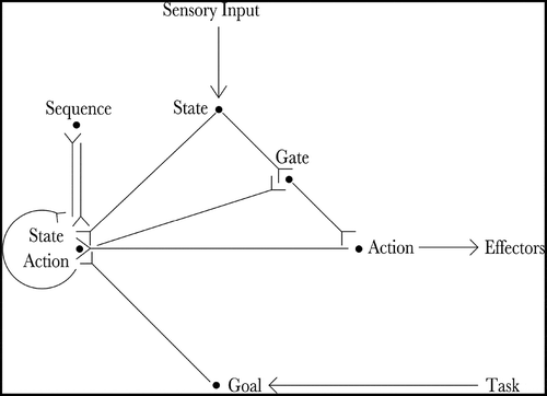
The proposed neural architecture is described by Figure 1. Essentially, the agent’s current state is input by the state cells and the agent’s goal is input by the goal cells. The state-action cells and the sequence cells co-operate to produce an action that will move the agent towards its goal. The gating cells read out the planned action and propagate it to the action cells, which produce movement.

Figure 1. The figure shows the architecture of the proposed hierarchical neural network model. The current state of the agent is input by the state cells (State) and the goal of the agent is input by the goal cells (Goal). Actions that moves the agent towards its goal are produced by the co-operation of the state-action cells (State Action) and the sequence cells (Sequence). Finally, the planned action is read out by the gating cells (Gate) and propagated to the action cells (Action), which produce movement

Map representation – State-Action (SA) cells

We hypothesize that, for a cognitive map to be useful for the production of actions, it should record how the actions of an agent in different states cause the agent to move between states. In Markovian terms, a cognitive map should encode the state transition probabilities within the environment.

For the sake of simplicity, we initially assume that transition probabilities are always 100%. Sec. 4.4 demonstrates planning when this is not true.

We therefore hypothesize that the proposed model encodes this information in terms of state-action combinations and it follows that the network should encode information using a neural substrate of SA cells, each of which encodes a unique combination of one state and one action.⁶

If SA cells respond to a combination of state and action information, they are therefore most likely to occur in an area which receives high-level sensory and motor feedback. The prefrontal cortex is located in the right part of the sensorimotor pathway and prefrontal cells are activated by stimuli from all sensory modalities, before and during a variety of actions, and in anticipation of expected events and behavioural consequences (Wallis et al. 2001). They are also modulated by motivational state (Wallis et al. 2001). Prefrontal neurons also output to the premotor cortex, which is known to represent and perform high-level actions (Tanji and Hoshi 2008).

In general, the prefrontal cortex is considered to be responsible for executive function at the top of the motor hierarchy (Fuster 2001). Lesions of lateral prefrontal cortex produces an inability to generate novel or complex sequences of behaviour, and patients find it difficult even to consciously represent such sequences, indicating that the lateral prefrontal cortex is at least necessary for generating such sequences and may contain the substrate which represents them (Fuster 2001).

More specifically, single-neuron recordings have shown that over the course of a task, cells in the primate prefrontal cortex come to represent and respond to combinations of sensory cues and motor actions by a process of associative learning (Asaad et al. 1998). Later work has strongly suggested that abstract and hidden states are represented in the orbitofrontal cortex (Wilson et al. 2014; Schuck et al. 2016) and recent work has found that cells in the rat orbitofrontal cortex encode a mixture of stimulus and choice information about the rat’s previous decision (Nogueira et al. 2017).

Map representation – minicolumns

We further hypothesize that these state-action cells are likely to be organized into minicolumns. These are stereotyped structures commonly found throughout the neocortex, usually with approximately 80–100 neurons, and are subject to an array of cortical inhibitory interneurons (Buxhoeveden 2002). This allows a variety of inhibition to occur within and between minicolumns, with very different levels of specificity and suppressive effect. We propose that such inhibition plays an important part in the formation of SA cells (see Sec. 4) and allows activity to be controlled and sustained during planning (see below). In this paper, the term “column” refers to a minicolumn unless otherwise stated.

In the proposed model, the state-action cells are structured into state columns. Each of these state columns contain several state-action cells which respond to the same state but to different actions (e.g. movement north, south, east and west) taken within that state. Section 4 shows how the state column structures can naturally self-organize using lateral inhibition within columns.

Map representation – encoding backward causal models using recurrent connectivity

One way that a layer of state-action cells can encode the topology of an environment is in the recurrent connectivity between them. If each state-action cell encodes a certain state-action combination possible in the environment, transitions can therefore be encoded in the recurrent weights between cells encoding a state-action and cells encoding the resultant successor state. If this recurrent connectivity is extensive enough, the network as a whole would encode the topology of the state space. Furthermore, activity propagating through the layer of state-action cells would do so according to the pattern of recurrent connectivity and so would be influenced by its topology, allowing planning.

In the model described below, the recurrent connectivity between these state-action cells encodes a backwards causal model of the environment; such a model encodes how each state can be reached as the result of performing particular state-action combinations. This is in contrast to a forward causal model that encodes the reverse information: the predicted results of performing certain state-action combinations. Another way of thinking about this is that a forward model records how causes produce effects, and therefore models the causal relationship forward in time, while a backward model records how effects are produced by causes, and therefore models the causal relationship backwards in time.

This distinction is significant because it determines what kind of information the model stores and is able to output. A backward causal model is able to give a set of state-action combinations that will lead to a desired state, but cannot output predictions about the result of performing any given state-action combinations. A forward model is the opposite.

A navigating model receives a desired end goal at the beginning of a task and is then required to output actions in order to move an agent from its current state to the desired state. The format of a backwards causal model is much more suited to this task and so we hypothesize that the planning mechanism in the brain uses a backward causal model.

As stated previously, we have hypothesized that the model encodes causal relations between states by means of synaptic connectivity between state-action cells. Because we have also hypothesized that these causal relations are encoded using a backwards causal model, the hypothesized connectivity must reflect that. A state-action cell $(s,a)$ that moves an agent into a new state $s\mathrm{\prime }$ therefore receives an excitatory synapse from any state-action cell that encodes that new state, so that activity can propagate backwards from the desired state to identify suitable state-action combinations to bring about that state. We have illustrated the proposed connectivity between state-action cells in Figure 2.

Figure 2. The pattern of connectivity between SA Cells encoding a reverse causal model. All SA cells within a given column encode the same state, and each SA cell encodes a different state-action combination. We hypothesize that each SA cell should receive a set of afferent synapses from all of the SA cells encoding its predicted successor state, allowing cells in a successor state to activate the SA cell responsible for entering that successor state. Likewise, each SA cell sends an efferent synapse to any SA cells that will result in the SA cell’s own encoded state

Map-based planning

A cognitive map is encoded by the strengthened recurrent connections within the layer of state-action cells. The proposed network feeds goal signals into the state-action layer at the goal location and allows these signals to propagate outwards through the topological connectivity of the cognitive map.

This propagation through the cognitive map is the primary element of the planning process. The quickest path to take from the agent’s current state to the goal location is that requiring fewest state transitions. Since each state-action cell represents, in effect, a state transition, the path requiring fewest state transitions will also be the path that activates fewest state-action cells between the agent’s current state and the goal location.

A common mechanism in the literature is to use decaying propagation, so that some activity is lost every time activity propagates between state-action cells. Consider a goal signal propagating through the recurrent connections towards the state-action cells associated with the current state of the agent. In this decaying-activation paradigm, the optimal state-action cell for each current state is connected to the goal location via the fewest state transitions and so receives the least-decayed activation; in other words the most active state-action cell for each state will move the agent towards the goal fastest. However, this mechanism has the important limitation that the activity will eventually decay to a negligible level and so this mechanism (in a naïve form) is unable to plan over a sufficiently long distance.

The proposed model uses an alternative mechanism to identify the fastest path to the goal. This mechanism plans using the timing of goal-based activity propagation through cells encoding the cognitive map, rather than how much activation those cells receive. We do not hypothesize that activity decays as it propagates through the state-action layer. Instead, we hypothesize that activity will propagate along the shortest path to the goal fastest, because that path involves the fewest state transitions and so the activity does not have to transfer through very many state-action cells. The relative values of different actions in each state – the speed with which those actions move the agent towards the goal – are therefore determined by the temporal order in which those SA cells receive activation from the goal and become active.

The first SA cell to receive activation in each state now represents the optimal action to take in each state, and the level of activation is not relevant. This allows the level of activation to be kept at a constant level as the wave propagates through the map, allowing it to plan over longer distances. This mechanism also does not require time for activity to “settle” in the layer, or for cells to integrate activity.

This mechanism owes inspiration to work by Ponulak & Hopfield 2013 (Ponulak and Hopfield 2013). Their paper described a model in which a wave of activity propagates through a 2D layer of topologically organized pure state cells (neighbouring state cells were recurrently connected) and showed that this wave carried information about the direction of the goal. Specifically, if the goal is east of a state cell, the wavefront will “hit” the state cell from that direction. Ponulak showed that an anti-STDP mechanism could record this information in the recurrent synaptic connectivity of the layer by strengthening the synapses between cells to indicate the direction from which they were “hit” by the wave.

The mechanism that we have proposed retains the insight that the propagation of a wavefront can carry information about the direction of a goal, but uses this information in a rather different way. Rather than use a propagating wavefront to adjust the synapses between pure state cells and thus produce a synaptic vector field, we have proposed that a propagating wavefront can identify and output the most valuable state-action combination for a given state.

The proposed mechanism is therefore able to improve on the mechanism described by Ponulak & Hopfield in several key ways. Firstly, because the proposed planning mechanism is able to work in a state-action map, it is able to output explicit actions that move the agent towards the goal (see Output below). Secondly, because the proposed planning mechanism is able to perform planning without requiring a period of synaptic plasticity, it seems likely that an agent using this mechanism would be able to plan more quickly, and would not have to “undo” the new synaptic weights if there is a change in the goal state or the transition structure of the environment. Thirdly, because the proposed planning mechanism is able to plan without altering the synaptic weights that encode the cognitive map, we can store information in these weights. We show in this section that the proposed planning mechanism is able to interface with a mechanism for producing hierarchical behaviour.

Output

The proposed network is able to read off the optimal action at the current state from the planning process using biologically plausible neural mechanisms. An action read-out mechanism must perform two important roles. It must read out the recommended action for the current state whilst not reading out anything associated with any other states, a problem illustrated in Figures 3 and 4. In the case of the proposed network shown in Figure 1, this is effected by a set of gating cells that propagate activity from the appropriate section of the cognitive map (that which represents the current location of the agent) to the action cells, where it produces motor output. The gating cells are under heavy inhibition such that they can only produce firing if they are receiving both SA and state input, meaning that they only pass on activity from an SA cell when that SA cell matches the current state.

Figure 3. Illustration of the problem of reading out the correct action for the current state. (a) shows the firing rates of a layer of SA cells partway through a planning task. Each compass plot in (a) represents the firing rate of all SA cells which encode a particular state as illustrated in (b). The golden state is the goal location and the boxed state is the agent’s current state. The planning wavefront has activated a large number of SA cells, most of which encode an action (NW, SW, W) that will not move the agent towards the goal. The model cannot therefore simply sum or average the activity in the SA layer but has to gate this activity by the current state of the agent before it is passed to the action output layer. Furthermore, this read-out must happen at a specific time

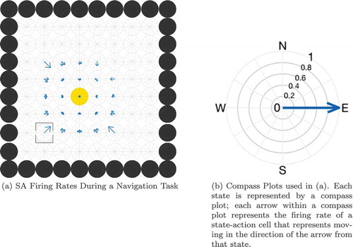
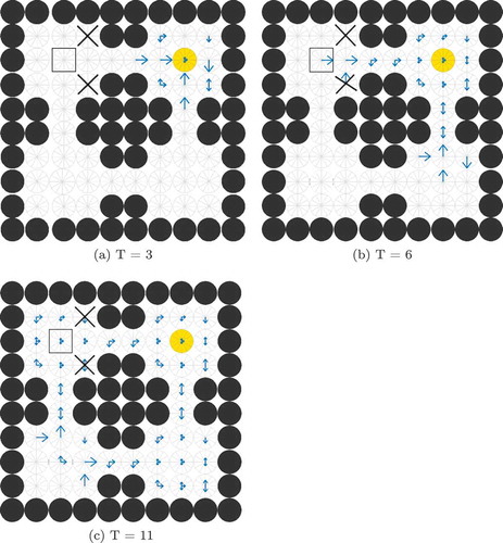
Figure 4. The Gating Problem. This figure shows compass plots of state-action activity during planning at three different times T = 3, 6 and 11. If the agent is occupying the state marked by the square, then the model should only read out activity from the SA cells marked by the square, and not (for example) those marked by crosses. Also, the agent should not read out activity from the marked SA cells at t = 3 (when the wave of activity has not yet reached the agent’s state) or at t = 11 (when the wave of activity has passed the agent’s state) but only at t = 6

Hierarchy

As explained above, the wave-propagation planning mechanism used by the proposed model relies exclusively on the timing of goal-based activity propagation through cells encoding the cognitive map, rather than how much activation those cells receive. The first SA cell to receive activation in each state represents the optimal action to take in that state, and the level of activation is not relevant. Since the model does not require time for the activity to “settle”, or for cells to integrate activity, the main factor limiting planning time is the speed of wavefront propagation. By increasing the speed at which activity propagates through the network, the planning process can be made much faster, provided that the spread of activity still produces viable plans. We hypothesize that frequently-used sequences of state-action combinations can act as shortcuts through state space, allowing activation to spread faster and further without sacrificing planning power.

Such a hierarchical planning mechanism would influence the model’s choice of actions during planning. As explained above, the speed of activity propagation through the recurrent connections of the SA layer is used to determine optimal routes during planning. If frequently-used sequences of state-action combinations are used to speed up the propagation of activity, these familiar sequences may be selected in preference to an optimal route. The preference for known routes has been observed in experimental studies (Brunyé et al. 2017; Payyanadan 2018). The model might also display this habitual behaviour in non-navigation tasks.

The use of “shortcuts” through the SA layer might also make planning more robust to noise, since transmission of activity between neurons is a primary source of noise and the use of shortcuts is intended to significantly reduce the number of transmissions of activity between SA cells. However, since the activity of SA cells in active columns is kept constant, and since planning in the model is dependent on the timing of activation propagation rather than on the precise activation value of SA cells, the effect of the hierarchical mechanism on planning in noisy conditions would likely be relatively small. Please note that the term “column” refers to cortical minicolumns (Buxhoeveden 2002) unless otherwise specfied.

We hypothesize that this hierarchical planning mechanism can be implemented by an extra layer of cells, called sequence cells, (Figure 1) whose connectivity to the state-action layer allows them to represent frequently used sequences of actions. These sequences encode behaviourally useful sequences which provide relatively direct routes through the state space. In determining the most likely form of sequence representation, there are two primary concerns:

1. A sequence cell must represent a useful sequence of state-action combinations. To do this, it must be linked to a particular set of state-action cells that represent a behaviourally useful sequence.

2. The planning mechanism implemented by the state-action cell layer should be able to call up and use sequences during the planning process. In other words, state-action cells must be able to activate sequence cells at an appropriate time – via the synapses from state-action cells to sequence cells – and sequence cells must be able to influence the activity of state action cells, via the synapses from sequence cells to state-action cells.

We hypothesize that a sequence cell (representing a sequence of state-actions) should be activated when the propagating goal-centred wavefront reaches the end of that sequence⁷ and should in turn activate the rest of the SA cells in that sequence immediately. This means that the wave can propagate through a sequence of $n$ state-actions (which would normally take $n$ timesteps) in 2 timesteps: one timestep for activity to propagate to the sequence cell, causing it to fire, and another timestep for that sequence cell to activate all of the $n$ SA cells that it is connected to.

As explained above, the time taken to output an action is dependent on how quickly the SA wavefront propagates from the goal to the agent’s current position. Put briefly, since the optimal action for each state is encoded by the state-action cell linked to the goal location by fewest transitions (and so fewest synapses), a wave of activity beginning at the goal and propagating at a constant speed will reach the optimal state-action cell before the rest of the state-action cells linked to that same state. The gating cells detect this activation and express the appropriate action to the action cells, which produce motor output.

As such, we hypothesize that incorporating sequence cells into the network model should enable the agent to plan a route of a given length in less time. Furthermore, because the speed at which activity propagates through a sequence does not depend on the length of the sequence, we hypothesize that the agent should receive larger gains in larger and more complex routes, where the path lengths are longer and thus the required planning time (without sequences) is longer.

Task

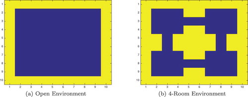
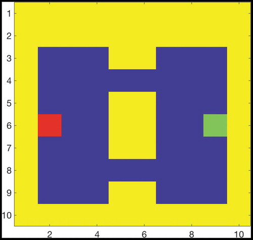
The agent is placed at a random position in one of four grid worlds. Two of these worlds are the small (10x10) open and maze worlds depicted by Figure 5. The other two worlds are the same but scaled by 2:1, so that they are 20 × 20. The agent can move one space at a time in eight compass directions⁸ or stay still, giving nine possible actions.

Figure 5. The 2-dimensional grid-world state space used to test the simulated network agents. The agent can move between blue squares, which are free states, and cannot move into yellow squares, which are walls. Each state has a unique index value which is used to fire a specific state cell

A random state is designated as the goal and the agent is required to navigate to this state to complete the task. If the agent reaches the goal location then the task has been been completed successfully. The number of timesteps required to reach the goal is recorded, as is the number of physical actions.

A set of 100 tasks is performed in each of the four environments, by two agents. The first agent has access to a set of sequence cells that encode various trajectories through the environment. The second agent has no access to sequence cells.

Model equations

The proposed model’s architecture is depicted in Figure 1 and contains:

• State cells

• Goal cells

• State-action (SA) cells

• Gating cells

• Action cells

• Sequence cells

Algorithm 1 Planning in the Hardwired Model with Sequence Cells. This describes the network’s operations during one timestep in the planning process. Steps in brackets only occur if there is activity in the action cell layer (signifying that an action has been selected for the agent’s current state).

Cell Firing State Cells & Goal Cells Fire

Activity Propagation SA Cells to Sequence Cells (1)

Activity Propagation SA Cells, Goal Cells & Sequence Cells to SA Cells (3)

Inhibition SA Cells: Rescale SA Activity in All Active States (4)

Activity Propagation State Cells & SA Cells to Gating Cells (5)

Inhibition Gating Cells: Threshold (6)

Activity Propagation Gating Cells to Action Cells (7)

Inhibition Action Cells: Winner-Take-All (8)

(Agent) Agent Moves to Successor State

(Reset) All Cells Reset to Zero Activation

Algorithm 1 describes one timestep of the planning process. The state cells fire, encoding the current location of the agent. These cells are one-hot: each state cell uniquely represents a single state and only one state cell fires at a time, denoting the current state. These cells are stimulated automatically, and are considered to be the output of unmodelled sensory processes. At the same time, the goal cells fire, encoding the desired state to be navigated to (i.e. the goal).

Activity spreads out from the goal location through the SA layer as a propagating wave. During this process (at every timestep) there is back-and-forth propagation of activation from the SA layer to the sequence layer (Equation 1(1) $h_i^{SQ}=\sum _j{w}_{ij}^{SA-SQ}{r}_j^{SA}$(1) ) and back to the SA network (Equation 3(3) $h_i^{SA}=\sum _j{w}_{ij}^{GL-SA}{r}_j^{GL}+\sum _j{w}_{ij}^{SA-SA}{r}_j^{SA}+\sum _j{w}_{ij}^{SQ-SA}{r}_j^{SQ}$(3) ). The sequence cell sends synapses to all SA cells in the sequence, but only receives synapses from the last SA cell in the sequence.

Sequence cells receive activation propagated from the SA cell layer as follows:

(1) $h_i^{SQ}=\sum _j{w}_{ij}^{SA-SQ}{r}_j^{SA}$(1)

(2) $r_i^{SQ}=h_i^{SQ}$(2)

where $r_j^{SA}$ is the firing rate of SA cell $j$ and $w_{ij}^{SA-SQ}$ is the synaptic weight from that SA cell to a sequence cell $i$, and these sequence cells – when active – pass activation back to the SA cells according to Equation 3(3) $h_i^{SA}=\sum _j{w}_{ij}^{GL-SA}{r}_j^{GL}+\sum _j{w}_{ij}^{SA-SA}{r}_j^{SA}+\sum _j{w}_{ij}^{SQ-SA}{r}_j^{SQ}$(3) .

SA cells are stimulated by a combination of goal input, recurrent SA activity and input from sequence cells as follows:

(3) $h_i^{SA}=\sum _j{w}_{ij}^{GL-SA}{r}_j^{GL}+\sum _j{w}_{ij}^{SA-SA}{r}_j^{SA}+\sum _j{w}_{ij}^{SQ-SA}{r}_j^{SQ}$(3)

where ${\sum }_j{w}_{ij}^{GL-SA}{r}_j^{GL}$ is the input received from the goal cells, ${\sum }_j{w}_{ij}^{SA-SA}{r}_j^{SA}$ is the recurrent SA input, and ${\sum }_j{w}_{ij}^{SQ-SA}{r}_j^{SQ}$ is the input from the sequence cells (see below). SA cells experience divisive inhibition, rescaling the activity of SA columns so that each currently active column is rescaled to sum to 1, and each inactive column remains inactive (with a sum of 0):

(4) $\sum _i{r}_i^{SA}=\left\{\begin{array}{cc}1& {\sum }_i{h}_i^{SA}>0\\ 0& {\sum }_i{h}_i^{SA}=0\end{array}\right.$(4)

where ${\sum }_i{h}_i^{SA}$ is the sum of the activations of all SA cells in a given column.

A layer of gating cells has been hardwired such that each gating cell receives afferent synapses from one state cell and one state-action cell, and sends synapses to one action cell.⁹ Activity propagates to the gating cells as follows:

(5) $h_i^G=\sum _j{w}_{ij}^{S-G}{r}_j^S+\sum _j{w}_{ij}^{SA-G}{r}_j^{SA}$(5)

The gating cells are under heavy inhibition such that they can only produce firing if they are receiving both SA and state input:

(6) $r_i^G=\left\{\begin{array}{cc}{h}_i^G& h_i^G>t^G\\ 0& h_i^G\le t^G\end{array}\right.$(6)

where $t^G$ is a thresholding constant.

Activity propagates from the gating cells to the action cells as follows:

(7) $h_i^A=\sum _j{w}_{ij}^{G-A}{r}_j^G$(7)

(8) $r_i^A=\left\{\begin{array}{cc}{h}_i^A& h_i^A>t^A\\ 0& h_i^A\le t^A\end{array}\right.$(8)

where $h_i^A$ is the activation of an action cell $i$, $w_{ij}^{G-A}$ is the weight of a synapse from a gating cell $j$ to that action cell, $r_j^G$ is the firing rate of gating cell $j$ and $r_i^A$ is the final firing rate of the action cell after thresholding inhibition using the constant $t^A$.

The thresholding inhibition (Equation 8(8) $r_i^A=\left\{\begin{array}{cc}{h}_i^A& h_i^A>t^A\\ 0& h_i^A\le t^A\end{array}\right.$(8) ) has the effect of preventing any action cell from firing unless it is strongly stimulated by a gating cell. If any action cell begins to fire despite this inhibition, winner-take-all inhibition is applied to the action cell layer to select a single action. The agent takes the action represented by the winning action cell (i.e. it moves one space in the specified direction) and updates the world. The firing rate of all cells is then reset to zero.

This section is focused on investigating the mechanism of planning and the role that sequence cells may play in the planning process. We therefore do not discuss how the synapses in this model self-organize: the self-organization of the basic network is covered by Section 4, while the following Section 5 will discuss the self-organization of connectivity between the state-action layer and the sequence cell layer. The diagram in Figure 1 depicts the overall architecture of the model, and Table 1 gives relevant model parameters.

Table 1. Table of parameters for the hardwired model with sequence cells described in Section 3

Parameter	Value
Action Cell Threshold t^A$t^A$	0.2
Gating Cell Threshold t^G$t^G$	0.55

Results

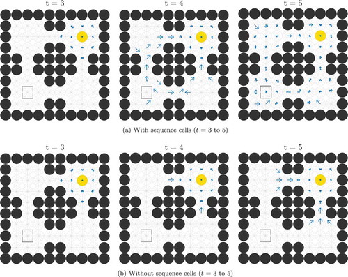
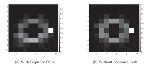
If a given sequence cell projects efferent synapses to all of the SA cells in a sequence but only receives an afferent synapse from the last SA cell in the sequence, that sequence cell will become active if the last SA cell in the sequence that it encodes becomes active. It will then immediately activate all of the other SA cells in that sequence. In effect, it allows the propagating wave to “skip” those cells, propagating through the entire sequence at once. This allows the propagating wave to travel faster through certain areas of state-action space, an effect demonstrated in Figure 6, which shows the same navigation task with and without connectivity between the SA and sequence cells. In effect, the sequence cells have produced a two-level hierarchical planning mechanism, where planning happens on the level of individual state-actions but also on the level of larger state-action sequences.

Figure 6. This figure shows the propagation of activity from the goal location through the SA layer during a simulated navigation task in the four-room environment shown in Figure 5(b). Results are shown for simulations with and without sequence cells. Each state is represented by a compass plot which depicts the activity of the SA cells representing that state (see Figure 3(b)). The golden state represents the goal, and the boxed state represents the agent’s current location. The agent moves once activity reaches its current state. We see that activity propagates considerably faster when sequence cells are available – compare (a) vs (b) – and that the propagating activity therefore reaches considerably more states after five timesteps

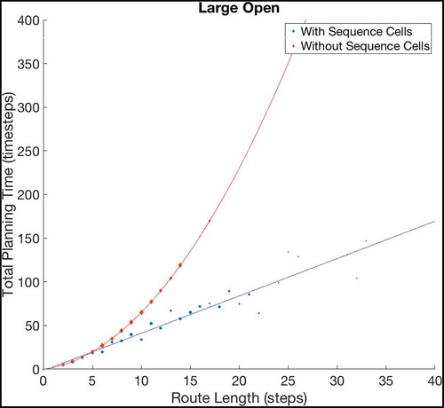
Figure 7 shows the effect of using or not using sequences on tasks with different path lengths. We see that use of the sequence cell mechanism has relatively little effect on short paths, but provides a significant (^~40–60%) decrease in total planning time on path lengths of ^~10 steps. These gains continue to increase as path length and environment complexity increase. Figure 8 shows that the total planning time of the model seems to grow quadratically without the sequence mechanism and linearly when augmented with sequence cells.

Figure 7. A figure showing how the total planning time varies with navigation tasks whose solutions are of different lengths. Results are shown for open environments as illustrated in Figure 5(a) (left column) and 4-room mazes illustrated in Figure 5(b) (right column). This demonstrates that use of sequences in planning produces low efficiency benefits during short tasks but increasingly large benefits as the required route length increases

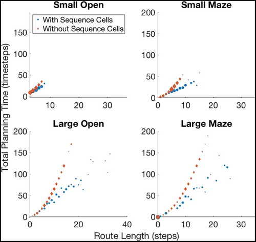
Figure 8. Fitting curves to the results of navigating within Large Open environments. The basic model, without using sequences, produces planning times that increase quadratically with the route length, while the augmented model, using sequences, plans linearly with the route length. Extrapolating these fits predicts that the gains should grow very large as the size and complexity of environments increase, although we cannot currently verify this claim as the discrete state-action representation we use does not scale well beyond 20 × 20 states (discussed further in Sec. 6.1). To check the accuracy of both fits, we have calculated the Adjusted-$R^2$ values for each fit. The Adjusted-$R^2$ is a statistical measure of how close the data are to the fitted lines, adjusted for the number of terms that describe the fitted line. These values are 1 for the model without sequence cells and 0.9243 for the model with sequence cells. The value of Adjusted-$R^2$ must be between 0 and 1, and so these values show that both lines fit the data extremely well

The kind of state spaces experienced by a mammalian intelligence (especially a primate one) are very much more complicated and thus larger than the state spaces used in this experiment, and problems in such large state spaces are difficult to solve using naive Markovian decision processes because the computation requirements in such environments are too large. The relationship between efficiency gains and environment size & complexity suggest that the efficiency gains would be much larger in real-life state spaces.

Figure 10 shows that if two paths of equal length exist from the agent’s starting position to its goal, then the hierarchical model incorporating sequence cells will tend to prefer familiar routes (those that have associated sequences) over other routes of equal distance. The model was trained in an 8 × 8 two-gate environment (Figure 9) and given a set of sequence cells encoding routes through the lower gate but not the upper gate. We see that the model is considerably more likely to choose the lower gate if it has access to these sequences. Note that the agent used probabilistic propagation (described more fully in sec. 4.4) for this planning task; this adds a nondeterministic element such that activity propagates from one cell to another with a given probability. Since the use of sequences to encode a route reduces the number of cells that activity must propagate through in order to choose that route, such a route has a higher probability of being chosen.

Figure 9. Two Gate Environment (8x8). As in Figure 5, the agent can move between blue squares, which are free states, and cannot move into yellow states, which are walls. The green square represents the goal, and the red square represents the agent’s starting state. The agent therefore starts equidistant from both gates, and can reach the goal from either gate in the same number of timesteps

Discussion

The hierarchical mechanism should be extensible to an arbitrary degree by adding more layers of sequence cells, such that higher layers learn sequences of sequences. This explains the observation that people plan on different scales and levels of abstraction (Klippel et al. 2003; Timpf and Kuhn 2003; Wiener and Mallot 2003) and are able to navigate over distances orders of magnitude apart, from short room-to-room movements within a house or workplace to long drives between cities and/or countries. These abilities have also been observed in bats, one of the few mammals whose large-scale navigation has been extensively studied. Bats have been observed to recall the three-dimensional position of objects with an accuracy of 1–2 cm but can also navigate reliably and regularly to targets dozens or thousands of kilometres away (Geva-Sagiv et al. 2015). Wild rodents have a similar range of navigational capabilities (Geva-Sagiv et al. 2015). We believe that although planning-time-to-path-length correlations seem to exist for problems of the same scale (Ward and Allport 1997; Howard et al. 2014), they do not seem to apply strongly to problems of different scales. For example, taxi drivers report being able to produce routes through London almost instantly (Spiers and Maguire 2008) even though these routes may be several kilometres in length.

The properties of the sequence cells depend on their connectivity with the state-action layer. The sequence cell should receive activity from the SA cell that occurs at the end of that sequence, so that the sequence cell will become active as soon as the activity wavefront reaches the end of the SA sequence. Likewise the sequence cell should be able to propagate activity to all SA cells in the sequence, so that it can quickly stimulate all of the SA cells encoding the sequence and thereby produce the maximal efficiency in planning. Self-Organizing mechanisms for learning this connectivity are described in Sec. 5. The sequences of actions that they encode are very similar to the high-level route segments described by Klippel et. al. (Klippel et al. 2003), and the action of the hierarchical mechanism utilizing sequence cells reproduces the fine-to-coarse planning heuristic described by Wiener and Mallot 2003 (Wiener and Mallot 2003). This hierarchical mechanism also appears to produce a preference for familiar routes – those for which the agent has available sequences – as seen in Figure 10. This preference has been experimentally demonstrated in human navigation (Brunyé et al. 2017; Payyanadan 2018). It also suggests that, in more complex tasks and environments, the hierarchical mechanism may produce a form of habitual behaviour, where inefficient but familiar solutions are preferred over optimal but planning-intensive solutions.

Figure 10. This figure compares the probability of an agent occupying various states in a two-gate environment (Figure 9) over the course of 100 planning trials. (a) shows these occupancy probabilities when the model has access to sequence cells that encode a route through the lower gate. (b) shows the same model without access to these cells. The agent is required to move from position (2,6) to (9,6), which can be achieved in the same number of actions by passing through either gate. We see that the existence of these sequences biases the agent to use the familiar lower gate rather than the higher gate in (a). By contrast, when the agent does not have access to these sequences it uses both gates with approximately equal probability (b)

Sequence cells in pre-SMA

Sequence-selective cells have been found in the supplementary motor area (SMA) and pre-supplementary motor area (pre-SMA). These cells fire before a particular (previously learned) sequence is performed but do not fire during the motor performance of that sequence (Shima and Tanji 2000). The pre-SMA is known to be connected to the prefrontal cortex (Luppino et al. 1993), allowing interactions between sequence cells in the pre-SMA and state-action cells in PFC to occur as seen in the model.

Figure 11 shows a simulated sequence cell firing during a modified version of the navigation task, and compares it to experimental recordings performed by Shima et. al (Shima and Tanji 2000). As in other navigation tasks, the agent must navigate from its starting location to the goal. In this case, however, the starting location and goal are chosen manually to ensure that the only route to the goal included the sequence encoded by the sequence cell. The figure shows the recorded firing rates of this sequence cell before, during and after the sequence of actions encoded by the sequence cell.

Figure 11. Comparison of a simulated sequence cell to a recorded pre-SMA cell. In both the simulated and recorded data, we see that the cell has strong firing before but not during a specific sequence of actions (a dashed line marks the onset of this sequence). However, the simulated data displays periodicity, unlike the recorded data. This is discussed in the main text. The proposed model is rate-coded and so the raster plot (a) was generated from recorded firing rates using a Poisson distribution

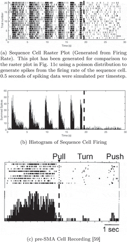
As explained in Section 3.1, the network plans by propagating goal-based activation through the SA layer and recording which of the state-action cells responsible for the current state receive activation first. Sequence cells function as “shortcuts” for the propagation of this wave. For this reason, the sequence cell will be strongly active before the agent performs the relevant sequence of actions. The propagating wave activates the sequence cell on its way to the agent’s current state, so that it becomes active early and remains active until the propagating wave reaches the agent’s current state. The activity then activates a gating cell and action cell as described by Sec. 3.3, and the agent takes an action that moves it towards the goal. The activity in the SA layer resets and the activity begins propagating again from the goal state.

This cycle of activity propagation and movement repeats until the agent reaches the first state that is involved in the sequence described by the connectivity of the sequence cell. Previously, the sequence cell was active for an extensive period of time while activity propagated further through the SA layer, beyond the sequence encoded by the sequence cells. However, SA cells responsible for the agent’s current location are now within the encoded sequence and so can be stimulated directly by the sequence cell without requiring further time for activity propagation. This means that as soon as the sequence cell becomes active, so do the relevant SA cells, gating cells, and action cells. The sequence cell is therefore only active very briefly when the agent is performing the sequence which the sequence cell encodes.

To put it another way, the sequence cell is only active after the propagating activity reaches the sequence cell’s preferred sequence and until that activity reaches the SA cell encoding the agent’s current state. All SA cells in the sequence become active simultaneously, so if the agent’s current state is in the encoded sequence, the sequence cell will only be active for a very short period of time because activity is not propagating further through the SA layer.

Figure 11(b) shows the simulated firing rate of the sequence cell, and Figure 11(a) shows a spiking raster plot with the spikes generated according to the firing rates by a poisson distribution for comparison to the experimentally recorded data in Figure 11(c). We can see that the sequence cells in the proposed model have similar properties to the pre-SMA cells recorded in this figure (Shima and Tanji 2000). Not only do they both encode a particular sequence of actions (Shima and Tanji 2000), but they become active immediately before the encoded sequence is carried out and then cease to fire as the sequence is performed. Furthermore, impairing either SMA or pre-SMA inhibits the ability of monkeys to perform the learned sequences of actions when cued, even though they retain the ability to perform any of those actions individually (Shima and Tanji 2000).

The main difference between the simulated data and recorded data is the periodicity seen in Figure 11(a,b). This periodicity arises from the fact that the simulated agent took several steps before the onset of the sequence, and so several “cycles” of activity occured as the activity spread out from the goal state to the agent’s location to plan the next action. There are several possible explanations for this difference.

Firstly, the model artificially resets activity in the SA layer after each single action during a movement sequence. This is a result of implementing a simplified discrete model. Further work with models that operate in continuous time may eliminate such periodic behaviour in the sequence cells.

Secondly, the recordings took place under different task conditions. The pre-SMA recording in Figure 11(c) was taken during a task in which monkeys were trained to perform three different movements, separated by short waiting times, in four or six different orders. The monkeys then reproduced one of these sequences several times based on visual cues. In other words, the sequences were not initiated as part of a goal-directed set of free movements, but as a cue-induced sequence. The difference in cell behaviour may therefore be partly task-based, accessing the same representations through a slightly different mechanism.

Self-organization of the basic network model without hierarchical planning

The previous experimental section of this paper described a neural network model for planning solutions to a navigation task in a simple grid environment. However, the synaptic connections in the above model simulations were pre-wired, with no explanations of how these connections might be embedded in the brain through learning. The question of how such a network should self-organize its synapses is not trivial. We break the process down into several parts: the self-organization of the SA cells in order to encode unique combinations of state and action, the self-organization of the recurrent connectivity between these SA cells in order to encode the structure of the environment, and finally the self-organization of the gating cells that output the results of planning to the action cells. We will discuss self-organization of the connectivity to and from the sequence cells (the hierarchical mechanism) in Section 5.

Formation of SA cells

During learning, the SA cells must form afferent connections from the state cells and action cells such that each SA cell learns to respond to a unique combination of state and action. Moreover, all possible combinations of state and action must be represented by an even distribution of SA cells. We hypothesized that the required connectivity may be set up by competitive learning. In this scenario, a layer of SA cells receive afferent connections from a mixture of state cells and action cells. These connections are modified by associative Hebbian learning as the network agent explores its sensory training environment. During this process, the layer of SA cells is put under heavy mutual inhibition, such that very few cells can fire at the same time. This inhibition means that cells’ receptive fields become distributed evenly across the input space, because each cell can only fire if it learns to respond to part of the input space that has not been “claimed” by other cells.

An agent’s state is usually defined by several pieces of (partially) independent information. In this case the neural representation of the state will be distributed, with multiple state cells active simultaneously. Moreover individual state cells will be active for multiple different states. For example, when making coffee, the amount and position of the coffee grinds are an important indicator of your state, but so is the position of the cup, the kettle, etc. It is therefore important to see whether the model can learn to represent states that are defined in this fashion. A simple way to do so is to replace the single one-hot state representation with an xy-coordinates representation, thus defining the state with two independent pieces of information.

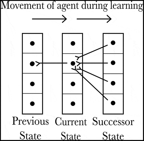
If the agent’s current state is $\left(\begin{array}{c}3\\ 4\end{array}\right)$ and it then moves west, encountering the state $\left(\begin{array}{c}4\\ 4\end{array}\right)$ for the first time, it will need to learn a new SA cell or state column to represent this new state. If there were only one piece of information, as in the previous sections, this would not be a problem: none of the existing SA cells have a connection to this new state, so the unused SA cells will compete to represent it. One of them will win that competition and thereafter will represent this new state. However, when the distributed xy-coordinate representation is used, there is already an SA cell that is partly associated with the state $\left(\begin{array}{c}4\\ 4\end{array}\right)$ because that state shares the same y-coordinate as the SA cell’s true state: $\left(\begin{array}{c}3\\ 4\end{array}\right)$. This “false” SA cell will therefore be more stimulated than the unused SA cells and will probably win the competition, either now representing both states or overwriting its previous associated state to represent this new state. Both are undesirable outcomes.

Hypothesis

We hypothesize that a competitive learning approach can be augmented using a columnar winner-takes-all mechanism to produce SA cells arranged in state columns from a distributed xy sensory representation, provided that inhibition is imposed to prevent SA cells from representing the current state if they are already associated with an overlapping state. This can be done using the bandstop inhibition described by Equation 10(10) $r_i^{SA}=\left\{\begin{array}{cc}{h}_i^{SA}& h_i^{SA}\le t_{min}^{SA}\\ 0& t_{min}^{SA}<h_i^{SA}<t_{max}^{SA}\\ h_i^{SA}& h_i^{SA}\ge t_{max}^{SA}\end{array}\right.$(10) . Such a mechanism will provide the columnar structure hypothesized by Sec. 3, such that a state column will form for each unique XY combination and therefore for each state.

Method

Algorithm 2 Self-Organizing SA Cells Using Competitive Learning with Distributed State Representations. This describes one timestep. All plasticity is Hebbian unless otherwise specified. The full sequence of events listed here occurs in every timestep.

Cell Firing State Cells

Activity Propagation State Cells to SA Cells (9)

Inhibition SA Cells: Bandstop Inhibition (10)

Inhibition SA Cells: Columnar Winner-Takes-All

Synaptic Plasticity State Cells to SA Cells (11 & 12)

Cell Firing Action Cells (13)

Agent Agent Moves to Successor State in Grid World

Activity Propagation State Cells & Action Cells to SA Cells (14)

Inhibition SA Cells: Full Winner-Takes-All (15)

Synaptic Plasticity State Cells & Action Cells to SA Cells (11, 12, 16 & 17)

Reset All Cells Reset to Zero Activation

Alg. 2 describes one timestep. The state cells fire, representing the current state. The state cells in this experiment have been modified to represent the agent’s state as a pair of x-y coordinates. The state layer consists of two sets of 10 cells, each encoding a coordinate from 1 to 10 using one-hot encoding. Activity propagates from the state cells to the SA cells:

(9) $h_i^{SA}=\sum _j{w}_{ij}^{S-SA}{r}_j^S$(9)

where $h_i^{SA}$ is the activation of a state-action cell $i$, $r_j^S$ is the firing rate of state cell $j$, and $w_{ij}^{S-SA}$ is the weight of the synapse from state cell $j$ to state-action cell $i$. The SA cells are subjected to bandstop inhibition:

(10) $r_i^{SA}=\left\{\begin{array}{cc}{h}_i^{SA}& h_i^{SA}\le t_{min}^{SA}\\ 0& t_{min}^{SA}<h_i^{SA}<t_{max}^{SA}\\ h_i^{SA}& h_i^{SA}\ge t_{max}^{SA}\end{array}\right.$(10)

where $h_i^{SA}$ is the activation of a cell $i$ in the SA cell layer, and $t_{min}^{SA}$ & $t_{max}^{SA}$ are constants that define the limits of the suppressed bandstop. Competition is applied across the SA layer in such a way that only one mini-column, representing a single state, remains active. Specifically, for each mini-column $c$ we compute the total activation across all of the SA cells in that mini-column according to $h^c={\sum }_i{h}_i^{SA}$. We then identify the mini-column with the largest value of $h^c$. The firing rates $r_i^{SA}$ of all cells in that mini-column are set to one, while the firing rates of all other cells in all other mini-columns are set to zero. As a result of this columnar inhibition, the firing rate $r_i^{SA}$ of SA cells in the minicolumn with the highest total activation is 1 while the rest are suppressed to 0. We will refer to this mechanism as “Columnar WTA”, standing for “columnar winner-takes-all inhibition”

The synapses between the state cells and the SA cells are updated:

(11) $\mathrm{\Delta }{w}_{ij}^{S-SA}=k{r}_i^{SA}{r}_j^S$(11)

where $k$ is a learning rate constant, $r_j^S$ is the firing rate of a state cell $j$ and $r_i^{SA}$ is the firing rate of a SA cell $i$. These synapses are then rescaled:

(12) $\sum _i{w}_{ij}^{S-SA}=t^{S-SA}\mathrm{\forall }j$(12)

where $t^{S-SA}$ is a constant.

Note that rescaling is used to bound synaptic weights instead of normalization because it produces more distinction between strengthened and unstrengthened synapses and allows for synapses to be bounded at arbitrary limits more straightforwardly.

A random action cell is activated:

(13) $r_i^A=1$(13)

where $r_i^A$ is the firing rate of a randomly chosen action cell $i$. The firing of this randomly-chosen action cell causes the agent to move in a corresponding direction from its current state. Activity propagates from the state layer and the action layer to the SA layer:

(14) $h_i^{SA}=\sum _j{w}_{ij}^{S-SA}{r}_j^S+\sum _j{w}_{ij}^{A-SA}{r}_j^A$(14)

The layer is then subject to full winner-takes-all inhibition:

(15) $r_i^{SA}=\left\{\begin{array}{cc}{h}_i^{SA}& h_i^{SA}={max}_i\left\{h_i^{SA}\right\}\\ 0& h_i^{SA}<{max}_i\left\{h_i^{SA}\right\}\end{array}\right.$(15)

where ${max}_i\left\{h_i^{SA}\right\}$ is the activation value of the most active cell in the SA layer. The synaptic weights between the action cells and the SA cells are updated:

(16) $\mathrm{\Delta }{w}_{ij}^{A-SA}=k{r}_i^{SA}{r}_j^A$(16)

and so are the synaptic weights between the state cells and the SA cells (Equation 11(11) $\mathrm{\Delta }{w}_{ij}^{S-SA}=k{r}_i^{SA}{r}_j^S$(11) ). Both sets of synapses are rescaled (Equation 12(12) $\sum _i{w}_{ij}^{S-SA}=t^{S-SA}\mathrm{\forall }j$(12) ) and:

(17) $\sum _i{w}_{ij}^{A-SA}=t^{A-SA}\mathrm{\forall }j$(17)

where $t^{A-SA}$ is a constant.

All cell activations are then reset for the next timestep. Table 2 shows all parameters that were added or altered from previous sections.

Table 2. Table of parameters for the model described in Section 4.1

Parameter	Value
Action Cell to SA Cell Rescaling ($t^{A-SA}$)	0.25
State Cell to SA Cell Rescaling ($t^{S-SA}$)	1
SA Cell Upper Threshold $t_{max}^{SA}$	1.5
SA Cell Lower Threshold $t_{min}^{SA}$	0.5
Learning Rate ($k)$	100

Results

We use an information-theoretic measure to test whether the model has correctly self-organized SA cell responses. This measure tests whether the response of an SA cell can be linked to a specific combination of state-action inputs. An SA cell has high single-cell information if its activity is sufficient to predict the presence or absence of a particular SA combination; in other words if that SA cell reliably responds to one state-action combination and reliably does not respond to any other state-action combination.

To generate this measure, we generate every combination of state-action that could be encountered in the environment on which the model was trained. This is every action, taken in every state that is not covered by a wall. (The blue area in Figure 5(a) contains 64 free states and so 64*9 = 576 state-action combinations). For each combination, the appropriate state cells and action cells are activated, and this activity propagates to the SA cells as in Equation 14(14) $h_i^{SA}=\sum _j{w}_{ij}^{S-SA}{r}_j^S+\sum _j{w}_{ij}^{A-SA}{r}_j^A$(14) . These cells were subjected to WTA inhibition (Equation 15(15) $r_i^{SA}=\left\{\begin{array}{cc}{h}_i^{SA}& h_i^{SA}={max}_i\left\{h_i^{SA}\right\}\\ 0& h_i^{SA}<{max}_i\left\{h_i^{SA}\right\}\end{array}\right.$(15) ). The responses of these cells are recorded and used to calculate the amount of information that each SA cell’s response gives about the stimulus. This is calculated as follows:

(18) $I(s,\vec{R})=\sum _{r\in \vec{R}}P(r|s){log}_2\frac{P(r|s)}{P(r)}$(18)

where $s$ is a particular stimulus (a particular state-action combination) and $\vec{R}$ is is the set of recorded responses of the SA cell. The maximum amount of information that an SA cell can carry is given by the equation $I_{m}ax=lo{g}_2(n)$ bits where $n$ is the total number of state-action combinations. Thus $I_{max}=lo{g}_2(576)=9.1699$ bits.

Figure 12 shows that the model is able to learn SA cells with full single-cell information even when the state is represented in a distributed manner by two pieces of independent information (the x- and y-coordinates). Furthermore, Figure 13 shows that each state-action combination is represented by an SA cell.

Figure 12. Single cell information learned by SA cells in a task using overlapped distributed xy representations of the agent’s state. Maximum information is indicated by the horizontal dashed line, and the maximum number of SA cells that can form without redundancy is indicated by the vertical dashed line

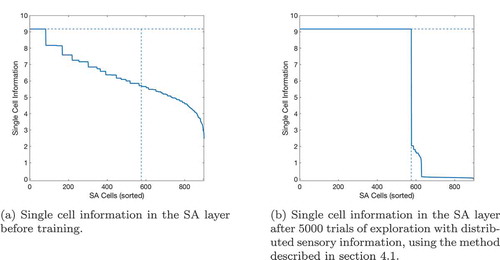
Figure 13. Firing of SA cells in a task using overlapped distributed xy representations of the agent’s state. The number of SA cells which fire for each state-action combination is recorded before and after training. (a) demonstrates that before training, a small number of SA cells will fire uniquely for one state-action combination (see also Figure 12(a)) due to the random initial synaptic connectivity between state cells, action cells and SA cells. A few state-action combinations are therefore uniquely represented by one SA cell before training. (b) then shows that after training, all state-action combinations are uniquely represented by one SA cell

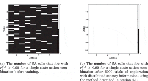
Figure 14 shows that the agent has explored more than half of an open 10 by 10 state map after ^~100 timesteps and almost every possible state after ^~500 timesteps. The agent will have learned to represent at least one state-action in each state and, assuming that the agent learns how they are connected at the same time as described in the next section, this means (assuming the presence of a read-out mechanism) that the agent should be able to form a (convoluted) path from almost any state to almost any other state after only ^~500 timesteps (Figure 21). However, it takes considerably longer (about 2000 timesteps) to fully learn all of the SA combinations available in the environment and so to learn all of the possible transitions between those states, which is required for optimal planning.

Figure 14. This figure records how many states (Figure 14(a)) and SA combinations (Figure 14(b)) are encountered when the agent is allowed to explore for different numbers of timesteps. It shows that the agent has explored more than half of an open 10 by 10 state map after ^~100 timesteps and almost every possible state after ^~500 timesteps

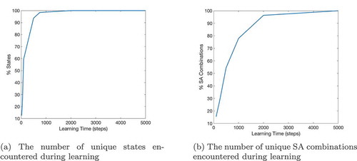
Discussion

The model is able to successfully form SA cells when the model uses overlapping distributed xy representations of the agent’s state. Successfully self-organizing SA cells using the method described in this section seems to require both a columnar winner-takes-all mechanism as well as a bandstop inhibition mechanism.

From a modelling perspective, the columnar winner-takes-all (columnar WTA) approach is useful because it naturally ensures the formation of state mini-columns. That is, if each SA cell encodes a combination of one state and one action, then for every state (position) there is therefore a vector of SA cells associated with that state, each representing a different action (direction of movement) that can be taken in that state. If the SA layer self-organizes such that SA cells representing the same state are drawn from the same mini-column (as in Hasselmo 2005 (Hasselmo 2005) and Martinet 2011 (Martinet et al. 2011)) then it becomes possible for inhibitory mechanisms to control the relative activity between states (by controlling the relative level of overall activity between mini-columns) whilst independently controlling the relative activity between different actions that can potentially be taken in each state (by controlling the relative activities of SA cells within the same mini-column).

In Section 3 we used this columnar structure to keep the level of activity in each active mini-column constant, allowing the propagating activity to spread through the SA layer without decaying. The columnar WTA learning model described in this section shows that state-action cells naturally self-organize into state columns given lateral columnar inhibition (which has been observed experimentally (Buxhoeveden 2002)). The Columnar WTA learning model is therefore able to form a structure that allows for easy management of the propagation of activation through the layer during planning. The requirement for different inputs (state, or state & action) and competition types at different points in each timestep is potentially concerning from the point of view of biological realism, however, as it is unclear how the specific order of events described in the simulation procedure for this experiment would be implemented in a more biologically realistic continuous-time model.

The primary problem that arises from using distributed sensory representations is that an SA cell which already encodes a state with a given x-coordinate or y-coordinate will be “unfairly” advantaged when competing to represent other states with the same x- or y-coordinate. Simple competitive learning may therefore fail to produce SA cells that only encode one state. Using only a columnar winner-takes-all mechanism may also fail for this reason, producing state columns that respond to more than one state. To learn a state representation in the task with distributed (XY) state representations therefore requires a method to prevent cells from “unfairly” competing. We have therefore chosen to use a bandstop inhibition mechanism.

An important point to note is that this section and the previous section have presented the model in two fundamentally different “modes” with fundamentally different dynamics. In the “planning” mode, described in Sec. 3, activity spreads outwards through the SA layer. This activity is constrained by normalizing the level of activity in each SA column. By contrast, in the “learning” mode described above, SA cells are subject to various forms of winner-takes-all inhibition such that only one SA column or one SA cell is active at any given time. The levels and types of inhibition are therefore fundamentally different between these two modes. Furthermore, the synapses between state, action, and SA cells are fixed during planning but are plastic during learning. These differences between the model’s learning and planning modes is necessary because the planning and learning modes require fundamentally different kinds of cell responses (a propagating wave vs. a single representative cell). Producing these different representations requires different inhibition. By the same token, allowing synapses to be plastic during the planning mode seems likely to lead to incorrect learning.

The next two sections describe how the model forms recurrent synapses between SA cells to encode the transition structure of the environment, and how the model learns the gating cells that are required for gating motor output during planning. The SA map learning mechanism is not directly affected by the state representation (provided that SA cells still form properly) and the gating cells form using competitive learning mechanisms similar to those described in this section.

Simultaneous Self-organization of state-action cells and a cognitive map encoded in the recurrent connections between them

Statement of problem

The overarching aim of this section is to explore how the cognitive map used to perform planning tasks in Section 3 might be learned in a biologically plausible fashion. The previous section successfully demonstrates that SA cells can learn to represent specific combinations of states and actions, even when sensory feedback is distributed and states are defined by multiple factors. However, in order to encode a full cognitive map, it is necessary not only to represent the states (or combinations of states and actions) within an environment, but also how an agent may transition between those states.

A number of previous models (Matsumoto et al. 2011) have tried to represent the topology of the environment within a layer of state cells by connected state cells that represent neighbouring states. Recurrent connectivity within the state layer then represents the topological structure of the environment. But this kind of state map is too simple for complex planning, especially in non-spatial tasks, because it does not encode the relationship between the agent’s own actions and state transitions. A map described purely in terms of state cells only describes the topology of the environment, and does not describe how an agent could produce actions to deliberately transition between states. In order to perform planning tasks we must also encode how specific actions lead to specific state transitions. In other words, we need to produce a causal map rather than a merely topological one. In this paper, we show that this form of map can be produced by utilizing a trace rule to learn a reverse causal model in the recurrent connections between state-action (SA) cells.

Hypothesis

We hypothesize that the a trace learning rule that incorporates a memory trace of neural activity in the postsynaptic cell can connect state-action cells that fire close together in time, producing various kinds of cognitive maps. In particular, we hypothesize that trace learning can produce connectivity as illustrated in Figure 2. This diagram shows how cells can encode an inverse causal model of the relationship between a successor state and the state-action combination which produces that successor state. That is to say, connections are strengthened from all of the SA cells representing the state that the agent ends up in to the SA cell that encodes the state-action combination that brings about that transition.

The self-organization of state-action cells was demonstrated in the previous section. This section will show a combined learning process that self-organizes SA cells to respond to particular state-action combinations (as in the previous section) whilst also learning a causal cognitive map in the recurrent connections between the SA cells as described above.

Task

An agent is placed in a 8 by 8 grid world, either an open environment or a 4-room maze, visible in Figure 5(a,b) respectively. During training, the agent was able to move in any of the eight cardinal directions or remain stationary. At each timestep, it chooses a random action and transitions to the appropriate successor state. The agent’s task is to explore the environment, self-organize SA cells to encode the state-action combinations that it experiences, and self-organize recurrent connectivity between these SA cells to encode the transitions that it experiences.

In other words, we expect that the agent, after training, should have recurrent connectivity between (self-organizing) state-action cells which represents the transitions available in the environment. If it does not – if the recurrent connectivity encodes transitions that do not exist in the environment, or if the recurrent connectivity fails to encode transitions that do exist in the environment – the agent will have performed poorly at this task.

Network model

The architecture of the network model used in this experiment is depicted in Figure 15. A layer of state cells encodes the current state of the agent within its environment. A layer of action cells encodes motor feedback about the action the agent has just taken. Both state and action representations use one-hot encoding in this experiment. A final layer contained potential SA cells.

Figure 15. Network architecture for learning a cognitive map in the recurrent connections between self-organizing SA cells

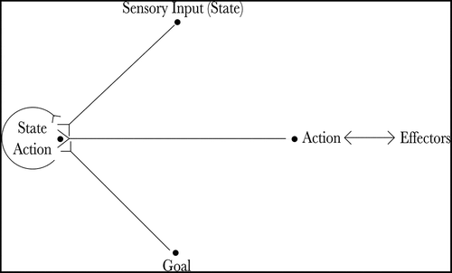
These SA cells receive full afferent connectivity from the sensory and action layers with initially random weights. The layer of SA cells is structured into a series of mini-columns. The number of these columns was made equal to the number of states and the number of cells in each column equal to the number of actions possible. The number of proto-SA cells therefore equalled the number of SA combinations necessary to learn. There is all-to-all recurrent connectivity between cells in the SA layer, but all recurrent synapses begin with a starting weight of zero.

Perceiving the current state

A specific sequence of events occurs in each timestep of the learning phase, as listed in Algorithm. The relevant parameters are listed in Table 3. First of all, a state cell fires, representing the current state. State cell firing is one-hot, so each state cell represents a single unique state and only one state cell is active at a time.

Algorithm 3 Self-Organizing SA Cells and Learning SA Map. This describes one timestep, expanded from alg. 2. The steps that have been added in this version are emphasized with italics. All plasticity is Hebbian unless otherwise specified. The full sequence of events listed here occurs in every timestep.

Cell Firing State Cells (Equation 19(19) $r_i^S=\left(\begin{array}{cc}1& i=\mathrm{c}\mathrm{u}\mathrm{r}\mathrm{r}\mathrm{e}\mathrm{n}\mathrm{t}\mathrm{s}\mathrm{t}\mathrm{a}\mathrm{t}\mathrm{e}\\ 0& i\ne \mathrm{c}\mathrm{u}\mathrm{r}\mathrm{r}\mathrm{e}\mathrm{n}\mathrm{t}\mathrm{s}\mathrm{t}\mathrm{a}\mathrm{t}\mathrm{e}\end{array}\right.$(19) )

Activity Propagation State Cells to SA Cells (20)

Inhibition SA Cells: Columnar Winner-Takes-All

Synaptic Plasticity State Cells to SA Cells (21 & 22)

Synaptic Plasticity Trace Learning: SA Cells to SA Cells (23 & 24)

Firing Action Cells (25)

Agent Agent Moves to Successor State in Grid World

Activity Propagation State Cells & Action Cells to SA Cells (26)

Inhibition SA Cells: Full Winner-Takes-All (27)

Synaptic Plasticity State Cells & Action Cells to SA Cells (21, 22, 28 & 29)

Synaptic Plasticity Set Memory Trace: SA Cells

Reset All Cells Reset to Zero Activation

(19) $r_i^S=\left(\begin{array}{cc}1& i=\mathrm{c}\mathrm{u}\mathrm{r}\mathrm{r}\mathrm{e}\mathrm{n}\mathrm{t}\mathrm{s}\mathrm{t}\mathrm{a}\mathrm{t}\mathrm{e}\\ 0& i\ne \mathrm{c}\mathrm{u}\mathrm{r}\mathrm{r}\mathrm{e}\mathrm{n}\mathrm{t}\mathrm{s}\mathrm{t}\mathrm{a}\mathrm{t}\mathrm{e}\end{array}\right.$(19)

where $r_i^S$ is the firing rate of a state cell $i$.

Table 3. Table of parameters for self-organizing model incorporating layer of SA cells described in Section 4.2

Parameter	Value
Input Learning Rate ($k^{IN})$	100
Trace Learning Rate ($k^{RC}$)	10

Activity propagates from the state cell layer to the SA layer, activating the SA cells in that layer as follows:

(20) $h_i^{SA}=\sum _j{w}_{ij}^{S-SA}{r}_j^S$(20)

where $h_i^{SA}$ is the activation of a state-action cell $i$, $w_{ij}^{S-SA}$ is the weight of a synapse from a state cell $j$ to that state-action cell, and $r_j^S$ is the firing rate of state cell $j$.

The potential SA cells in the SA layer are grouped in “mini-columns”. These mini-columns are analogous to the mini-columns used in certain alternative models.¹⁰ Each mini-column should self-organize to encode one and only one state, and so the number of mini-columns must be greater than or equal to the number of states to ensure that all possible state-action combinations are learned. Similarly, the number of state-action cells in each mini-column must be greater than or equal to the number of possible actions in each state.

Mini-columns are able to compete with all other minicolumns to fire, and competition is applied across the SA layer in such a way that only one mini-column, representing a single state, remains active. Specifically, for each mini-column $c$ we compute the total activation across all of the SA cells in that mini-column according to $h^c={\sum }_i{h}_i^{SA}$. We then identify the mini-column with the largest value of $h^c$. The firing rates $r_i^{SA}$ of all cells in that mini-column are set to one, while the firing rates of all other cells in all other mini-columns are set to zero. As a result of this columnar WTA inhibition, the firing rates $r_i^{SA}$ of SA cells in the minicolumn with the highest total activation are 1 while the rest are suppressed to 0.

Only one minicolumn is now active, and Hebbian learning is applied to the synapses $w_{ij}^{S-SA}$ that project from the input state layer to the SA layer as follows:

(21) $\mathrm{\Delta }{w}_{ij}^{S-SA}=k^{IN}{r}_i^{SA}{r}_j^S$(21)

where $k^{IN}$ is a learning rate constant, $r_j^S$ is the firing rate of a state cell $j$ and $r_i^{SA}$ is the firing rate of an SA cell $i$. These synapses are then rescaled so that:

(22) $\sum _i{w}_{ij}^{S-SA}=1\mathrm{\forall }j$(22)

The resultant strengthening of the synapses from the currently active state cell to the currently active SA minicolumn produces a state column: a pool of SA cells which are linked to a specific set of sensory cues representing a particular state (location), as described in Section 3.

Learning an inverse causal model

As seen in Figure 2, the learned recurrent connectivity between SA cells after learning should be many-to-one, such that an SA cell receives afferent synapses from every SA cell in its successor state. The required recurrent connectivity may be set up by applying a trace learning rule that incorporates a memory trace ${\bar{r}}_i^{SA}$ of neural activity in the postsynaptic neuron $i$. The memory trace can be computed in various ways. In this paper, we set the memory trace of a neuron on timestep $t$ to be equal to its firing rate in the previous timestep $t-1$. Thus, at this point in the timestep, the memory trace term ${\bar{r}}_i^{SA}$ encodes the SA cell that fired in the previous timestep, while the current firing of SA cells in the current state $r_j^{SA}$ encodes all SA cells in the successor state. The desired connectivity therefore occurs if the recurrent synapses between the cells in the SA layer are updated according to a trace learning rule as follows:

(23) $\mathrm{\Delta }{w}_{ij}^{SA-SA}=k^{TR}{\bar{r}}_i^{SA}{r}_j^{SA}$(23)

where $k^{TR}$ is a learning rate constant, ${\bar{r}}_i^{SA}$ is a memory trace of the postsynaptic SA cell $i$ where the memory trace ${\bar{r}}_i^t$ is set to be equal to the firing rate $r_i^{t-1}$ of the cell at the previous timestep $t-1$, and $r_j^{SA}$ is the firing rate of the presynaptic SA cell $j$. These synapses are then rescaled so that:

(24) $\sum _i{w}_{ij}^{SA-SA}=4\mathrm{\forall }j$(24)

The implementation of the trace learning rule 23 in the recurrent connections between the SA cells allows the network model to learn an inverse causal model of how the agent’s actions lead to transitions between states.

Taking an action

A random action cell is then stimulated manually as follows:

(25) $r_i^A=1$(25)

where $r_i^A$ is the firing rate of a randomly chosen action cell $i$.

The firing of this randomly chosen action cell causes the agent to move in a corresponding direction from its current state. The SA cells are now activated by a combination of state and action activity as follows:

(26) $h_i^{SA}=\sum _j{w}_{ij}^{S-SA}{r}_j^S+\sum _j{w}_{ij}^{A-SA}{r}_j^A$(26)

The state input that the SA cells are now receiving is the same as before, because the state cells have not yet updated. Cells in the SA layer have already formed synapses from the firing state cells (Equation 21(21) $\mathrm{\Delta }{w}_{ij}^{S-SA}=k^{IN}{r}_i^{SA}{r}_j^S$(21) ) and so the most active SA cells are those in the state column corresponding to the current state. A new form of winner-take-all inhibition is applied, which leaves only a single cell in the SA layer active:

(27) $r_i^{SA}=\left\{\begin{array}{cc}{h}_i^{SA}& h_i^{SA}={max}_i\left\{h_i^{SA}\right\}\\ 0& h_i^{SA}<{max}_i\left\{h_i^{SA}\right\}\end{array}\right.$(27)

where ${max}_i\left\{h_i^{SA}\right\}$ is the activation of the most active cell in the SA layer.

The incoming state cell input (Equation 26(26) $h_i^{SA}=\sum _j{w}_{ij}^{S-SA}{r}_j^S+\sum _j{w}_{ij}^{A-SA}{r}_j^A$(26) ) ensures that the most active SA cells in the layer are those representing the current state and so the SA cell which wins the competition to fire will be one from the relevant state column. Hebbian learning strengthens the afferent synapses that this cell receives from both the input state cells (through Equations. 21(21) $\mathrm{\Delta }{w}_{ij}^{S-SA}=k^{IN}{r}_i^{SA}{r}_j^S$(21) and 22(22) $\sum _i{w}_{ij}^{S-SA}=1\mathrm{\forall }j$(22) ) and input action cells through the following equations:

(28) $\mathrm{\Delta }{w}_{ij}^{A-SA}=k^{IN}{r}_i^{SA}{r}_j^A$(28)

where the synapses are then rescaled so that:

(29) $\sum _i{w}_{ij}^{A-SA}=0.25\mathrm{\forall }j$(29)

Through these strengthened connections from the sensory and action cells the SA cell has learned to be activated by the current combination of state and action.

At this point the firing rates ($r^{SA}$) of the SA cells are recorded and will become ${\bar{r}}_j^{SA}$ in the next timestep. The activity of all cells is then set to zero.

Results

To test the ability of the model to learn the transition matrix for its environment, we compare the model’s learned transition matrix (encoded in the recurrent synapses between SA cells) to the true transition matrix. We created the true transition matrix by algorithmically subjecting the agent to every combination of state and action that could be encountered in the environment on which the model was trained. This is every action, taken in every state that is not covered by a wall. (The blue area in Figure 5). We then recorded the state transition that occurred to produce the ground truth transition matrix.

After producing the ground truth transition matrix, we then decoded the recurrent synapses $w^{SA-SA}$ from the above experiment to derive the network’s own learned transition matrix. In the case of a cognitive map encoded in a layer of state-action cells, as described in this section, an encoded transition is a prediction that a state-action combination will produce movement to a successor state. In neural terms, a strong synapse from a presynaptic SA cell $i$ to a postsynaptic SA cell $j$ encodes a prediction that the state-action combination represented by SA cell $j$ will transition the agent to the successor state represented by presynaptic SA cell $i$. This connectivity is illustrated in Figure 2.

We decoded the recurrent connectivity in the SA layer to identify which predicted transitions were being encoded by these recurrent connections. This decoding process took place as follows.

Again, we generated every combination of state-action that could be encountered in the environment on which the model was trained. For each combination, the appropriate state cells and action cells are activated, and this activity propagates to the SA cells as in Equation 26(26) $h_i^{SA}=\sum _j{w}_{ij}^{S-SA}{r}_j^S+\sum _j{w}_{ij}^{A-SA}{r}_j^A$(26) . The firing rates of these cells was then rescaled so that all firing rates were between 0 and 1, and any SA cell which was firing at a rate > 0.99 was selected. These cells were considered to represent that state-action combination. We could then decode the agent’s learned transition matrix by analysing each synapse $w_{ij}^{SA-SA}$ and recording it as a transition from the state-action combination represented by SA cell $i$ to the state represented by SA cell $j$. We count a synapse as encoding a transition if its weight $w_{ij}$ is greater than $0.01$. The default value of such synapses before learning is $0$. Note that because the SA synapses encode a backwards model of the environment,¹¹ the direction of the synapse must be reversed to get the direction of the transition.

Having produced a ground truth transition matrix and a decoded learned transition matrix, we can compare the two to calculate the following terms:

• True positive (tp): a transition that appears in both the true and learned transition matrices. This is a possible transition that has been learned correctly.

• False positive (fp): a transition that appears in the learned transition matrix but not in the true matrix. This is a transition that the network thinks is possible but is not.

• True negative (tn): a transition that does not appear in the true or learned transition matrices. This transition is correctly understood to be impossible.

• False negative (fn): a transition that does not appear in the learned matrix but does appear in the true matrix. This is a possible transition that the agent has failed to learn.

Thus, $tp$ is the total number of true positives found when comparing the learned and ground truth transition matrices, $fp$ is the total number of false positives, $t_n$ is the total number of true negatives, and $fn$ is the total number of false negatives.

These terms can be used to calculate the precision (Equation 30(30) $\mathrm{P}\mathrm{r}\mathrm{e}\mathrm{c}\mathrm{i}\mathrm{s}\mathrm{i}\mathrm{o}\mathrm{n}=\frac{tp}{tp+fp}$(30) ) and recall (Equation 31(31) $\mathrm{R}\mathrm{e}\mathrm{c}\mathrm{a}\mathrm{l}\mathrm{l}=\frac{tp}{tp+fn}$(31) ) of the network. The precision represents the proportion of the learned transitions that are genuine (as opposed to false positives); the recall¹² measures the proportion of true transitions existing in the environment that the network has successfully learned. Figure 16 shows both measures for the model described in this section.

(30) $\mathrm{P}\mathrm{r}\mathrm{e}\mathrm{c}\mathrm{i}\mathrm{s}\mathrm{i}\mathrm{o}\mathrm{n}=\frac{tp}{tp+fp}$(30)

(31) $\mathrm{R}\mathrm{e}\mathrm{c}\mathrm{a}\mathrm{l}\mathrm{l}=\frac{tp}{tp+fn}$(31)

Figure 16. This figure shows the precision and recall achieved by the self-organizing columnar SA model described in Section 4.2. This model was run for 5000 timesteps of exploration in an open 8 × 8 environment. Precision and recall can vary between 0 and 1, and are plotted here as percentages. We observe that both precision and recall are at 100%. The model is able to represent all of the true transitions existing in the environment, and represents them all correctly

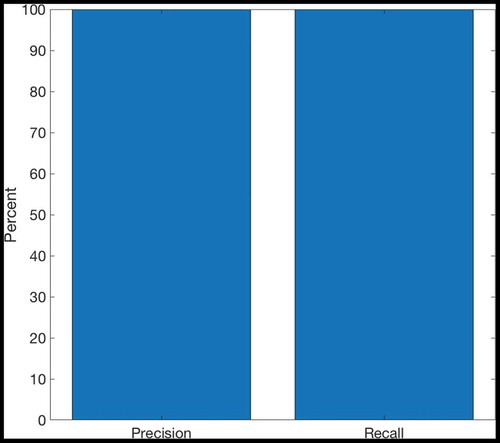
Discussion

Section 4.2 shows that trace learning is able to link SA cells in such a way as to store the topological relationships between states in the synaptic connectivity between these cells (Figure 16). At each timestep the network receives sensory & delayed action feedback and – if no SA cell already responds to this input combination – an SA cell learns to represent this combination. This SA self-organization is a two-step process, with a column of SA cells learning to represent the current state and one SA cell in that column learning to further respond to an action taken in that state. This means that the self-organization process produces a “state column” made up of SA cells that all respond to the current state.

The agent’s action transitions the agent into a new state (location) at the next timestep where it receives a new set of sensory cues, prompting the network to learn another “state column”. Trace learning strengthens recurrent connections to the single¹³ postsynaptic SA cell (representing the former state and the action that was taken in that state) from the SA cells in the mini-column representing the current state. This results in the many-to-one causal synapses we illustrated in Figure 2. The resultant network architecture encodes a causal cognitive map of its environment in terms of states and actions, such that it can plan using the inductive process described in Sec. 3.

Using a columnar architecture appears to be necessary for the planning stage but also greatly improves the efficiency of learning during exploration: the columnar WTA allows an SA cell to receive strengthened synapses from every SA cell in the resultant state (i.e. in the active state column), rather than simply the SA cell that is next to fire. The network described in this section has 9 possible actions that it can perform in each state and so using a columnar architecture will on average learn a full map after only experiencing 11% of the possible SA combinations.

The SA mapping mechanism described in this section relies on the use of a “memory trace” that allows a presynaptic neuron to continue strengthening synapses to a postsynaptic neuron even after the postsynaptic neuron has stopped firing (Equation 23(23) $\mathrm{\Delta }{w}_{ij}^{SA-SA}=k^{TR}{\bar{r}}_i^{SA}{r}_j^{SA}$(23) ). There are certain biological mechanisms that produce similar effects. In particular, experimental research has shown that cells which have previously experienced high firing rates may show increased excitability for some time afterwards, an effect which appears to be caused by the protein CREB (Rogerson et al. 2014). The raised excitability produced by CREB could potentially allow connections to form between SA cells that fire in succession, producing connectivity similar to that produced by a trace rule. CREB is often implicated in the formation of episodic memory traces. Evans and Stringer demonstrated a somewhat similar effect by extending the amount of time that postsynaptic activity or presynaptic activity takes to decay in a spiking cell model and showing that this allows these cells to remain active long enough to receive and associate several synaptic inputs in sequence (Evans and Stringer 2012).

The effects of CREB are not a perfect fit for the trace learning rule, however. CREB aids episodic memory formation by increasing the excitability of a cell that has previously fired, making it more likely to fire again in response to further stimuli. This is in contrast to the memory trace employed in the previous experiment, which allows a presynaptic neuron to continue strengthening synapses to a postsynaptic neuron even after the postsynaptic neuron has stopped firing. This allows the SA cell which fired in the previous timestep to strengthen its connections from the currently active SA column without strengthening its connections from the currently firing state and action cells. If the SA cell encoding the previous state-action combination remains active (due to CREB-based excitability) as the agent moves to the next state, we would expect it to start forming connectivity to this new state, interfering with the self-organization of a new SA cell.

The simulation procedure used in this section requires careful timing of inputs (as in Sec. 4.1), competition and trace formation/learning. Recurrent connectivity between SA cells is learned according to a function of present SA firing and previous SA firing (via a memory trace). This means that it is very important which cells are firing when the SA memory trace is calculated. To form the synapses from state-column to SA cell shown in Figure 2, the postsynaptic trace $\bar{r}$ must be set once WTA inhibition has produced a single SA cell for the previous timestep, but trace learning must occur while the whole state column is active for the current state.

Self-organization of gating cells using bandstop inhibition

Statement of problem

The question of how such a network should output and use the results of the plan produced in the SA layer is not trivial. To produce an action based on an internal planning process requires several linked mechanisms: firstly, the network must have a mechanism to determine when the planning process is complete to some degree of satisfaction; secondly, the network must have a mechanism to determine from the planning process what action is considered best to take in the current state. In other words, the network must read off the right action at the right time.

Most of the literature to date (Hasselmo 2005; Cuperlier et al. 2007; Martinet et al. 2011) posits that a gating mechanism is most suitable for this task. That is to say that an element of these models ensures than an action cannot be passed to the motor effectors unless a certain set of conditions are met. This gating mechanism is generally implemented as literal “gating cells” which receive input from both the sensory mechanism (representing the current state) and the planning mechanism, and which will only fire when they receive sufficient input from both. In other words, the signals from the route planning layer are gated by the current state of the agent before being passed to the action layer. These gating cells act as conduits of information from the planning mechanism to the motor effectors. However, there remains the question of how these gating cells acquire their distinctive connectivity (Figure 1) and properties.

Hypothesis

We hypothesize that the self-organization of the gating cells can be achieved by a form of competitive learning fundamentally similar to that of self-organizing state-action cells. This is because SA cells must also learn to respond to a specific combination of two inputs.

Task

An agent is placed in a 10 by 10 grid world (either an open environment or a small maze, shown in Figure 5(a,b) respectively). The agent is able to move in any of the eight cardinal directions. At each timestep, it chooses a random action and transitions to a new state. The agent’s task is to explore the environment and self-organize gating cells to encode the state-action combinations that it has experienced (along with SA cells as in the previous two sections).

We expect that the agent, after training, should have developed gating cells which respond strongly to an experienced state-SA combination. If it does not – if the gating cells respond exclusively to sensory inputs or exclusively to SA inputs, if the gating cells do not distinctly encode a single state-SA combination – the agent will have performed poorly at this task.

Network model

The architecture of the network is shown in Figure 17. A layer of state cells encode the agent’s current state using a one-hot encoding. A layer of action cells encode the action that the agent is taking or has just taken using a one-hot encoding. A layer of SA cells receive afferent synapses from the state layer and action layer. A layer of gating cells receive afferent synapses form the state layer and the SA layer. Where connectivity exists, it is all-to-all with random initial weights. The only exception is the recurrent connectivity within the state-action layer, which is all-to-all with zero initial weights, as described in Sec. 4.

Algorithm 4 Full Model with Self-Organization of Gating Layer. This describes one timestep, expanded from alg. 3. The steps that have been added in this version are emphasized with italics. All plasticity is Hebbian unless specified otherwise. The full sequence of events listed here occurs in every timestep.

Cell Firing State Cells (Equation 19(19) $r_i^S=\left(\begin{array}{cc}1& i=\mathrm{c}\mathrm{u}\mathrm{r}\mathrm{r}\mathrm{e}\mathrm{n}\mathrm{t}\mathrm{s}\mathrm{t}\mathrm{a}\mathrm{t}\mathrm{e}\\ 0& i\ne \mathrm{c}\mathrm{u}\mathrm{r}\mathrm{r}\mathrm{e}\mathrm{n}\mathrm{t}\mathrm{s}\mathrm{t}\mathrm{a}\mathrm{t}\mathrm{e}\end{array}\right.$(19) )

Activity Propagation State Cells to SA Cells (20)

Inhibition SA Cells: Columnar Winner-Takes-All

Synaptic Plasticity State Cells to SA Cells (21 & 22)

Synaptic Plasticity Trace Learning: SA Cells to SA Cells (23 & 24)

Firing Action Cells (25)

Agent Agent Moves to Successor State in Grid World

Activity Propagation State Cells & Action Cells to SA Cells (26)

Inhibition SA Cells: Full Winner-Takes-All (27)

Synaptic Plasticity State Cells & Action Cells to SA Cells (21, 22, 28 & 29)

Plasticity Set Memory Trace: SA Cells

Activity Propagation State Cells & SA Cells to Gating Cells (32)

Inhibition Gating Cells: Bandstop Inhibition (33)

Inhibition Gating Cells: Full Winner-Takes-All (34)

Synaptic Plasticity State Cells & SA Cells to Gating Cells (35, 36, 38 & 39)

Synaptic Plasticity Gating Cells to Action Cells (37 & 40)

Reset All Cells Reset to Zero Activation

Figure 17. Architecture of the proposed model with self-organizing gating layer

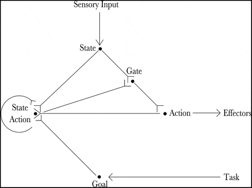
Algorithm 4 shows the sequence of events that happens in one timestep. Parameters are given in Table 4. We can see that the initial sequence of events (those not in italics) in each timestep is exactly the same as in algorithm, described in Sec. 4.2 At the end of this part of the process a single SA cell is active, as is a single state cell and a single action cell.

Table 4. Table of model parameters for Section 4.3

Parameter	Value
Gating Cell Upper Threshold $t_{max}^G$	1.5
Gating Cell Lower Threshold $t_{min}^G$	0.5
Gate Learning Rate ($k^G)$	100

Activity propagates from state cells and SA cells to gating cells, as follows:

(32) $h_i^G=\sum _j{w}_{ij}^{S-G}{r}_j^S+\sum _j{w}_{ij}^{SA-G}{r}_j^{SA}$(32)

where $h_i^G$ is the activation of a gating cell $i$, ${\sum }_j{w}_{ij}^{S-G}{r}_j^S$ is the activity contributed by state inputs and ${\sum }_j{w}_{ij}^{SA-G}{r}_j^{SA}$ is the activity contributed by SA inputs.

We then apply “bandstop” inhibition to the gating cells. This inhibits activity within a certain bandstop, inhibiting the mid-level activity typical of a gating cell which only partially represents current sensory-SA input. This prevents one gating cell from successfully competing for all state-SA combinations involving the same state, or all state-SA combinations involving the same SA combination, and so prevents the formation of single gating cells that respond to many state-SA combinations or gating cells that are constantly overwriting themselves. Bandstop inhibition takes place as follows:

(33) $r_i^G=\left\{\begin{array}{cc}{h}_i^G& h_i^G\le t_{min}^G\\ 0& t_{min}^G<h_i^G<t_{max}^G\\ h_i^G& h_i^G\ge t_{max}^G\end{array}\right.$(33)

where $h_i^G$ is the activation of a cell $i$ in the gating cell layer, $r_i^G$ is the firing rate of that cell and $t_{min}^G$ & $t_{max}^G$ are constants that define the limits of the suppressed bandstop.

After bandstop inhibition has been applied, winner-takes-all competition is applied by setting the firing rate of the most active gating cell to 1 and the firing rates of all other gating cells to zero as follows:

(34) $r_i^G=\left\{\begin{array}{cc}1& r_i^G={max}_i\left\{r_i^G\right\}\\ 0& r_i^G\ne {max}_i\left\{r_i^G\right\}\end{array}\right.$(34)

where ${max}_i\left\{r_i^G\right\}$ is the activity of the most active cell in the gating layer.

The synaptic weights between the state cells and gating cells are updated as follows:

(35) $\mathrm{\Delta }{w}_{ij}^{S-G}=k^G{r}_i^G{r}_j^S$(35)

and the synaptic weights between SA cells and gating cells are updated as follows:

(36) $\mathrm{\Delta }{w}_{ij}^{SA-G}=k^G{r}_i^G{r}_j^{SA}$(36)

and the synaptic weights between gating cells and action cells are updated as follows:

(37) $\mathrm{\Delta }{w}_{ij}^{G-A}=k^G{r}_i^A{r}_j^G$(37)

where $k^G$ is a learning rate constant.

These synapses are then rescaled so that:

(38) $\sum _i{w}_{ij}^{S-G}=0.5\mathrm{\forall }j,$(38)

(39) $\sum _i{w}_{ij}^{SA-G}=0.5\mathrm{\forall }j,$(39)

(40) $\sum _i{w}_{ij}^{G-A}=1\mathrm{\forall }j,$(40)

Results

To test the self-organization of gating cells we used an information-theoretic measure. This measure tests whether the response of a gating cell can be linked to a specific combination of state and SA inputs. A gating cell has high single-cell information if its activity is sufficient to predict the presence or absence of a particular state cell & SA cell combination; in other words if that gating cell reliably responds to one state cell & SA cell combination and reliably does not respond to any other state-SA combination.

To generate this measure, we generate every combination of state cell and SA cell that could be encountered in the environment on which the model was trained (every state that was not covered by a wall, combined with every cell in the SA layer). For each combination, the appropriate state cell and SA cell are activated, and the activity propagates to the gating cells as in Equation (32)(32) $h_i^G=\sum _j{w}_{ij}^{S-G}{r}_j^S+\sum _j{w}_{ij}^{SA-G}{r}_j^{SA}$(32) . We then thresholded the gating cells as follows:

(41) $r_i^G=\left\{\begin{array}{cc}{h}_i^G& h_i^G>t^G\\ 0& h_i^G\le t^G\end{array}\right.$(41)

where $t^G$ is a thresholding constant. We use thresholding (Equation 41(41) $r_i^G=\left\{\begin{array}{cc}{h}_i^G& h_i^G>t^G\\ 0& h_i^G\le t^G\end{array}\right.$(41) ) rather than the bandstop and WTA inhibition described earlier in this section (Equations 33(33) $r_i^G=\left\{\begin{array}{cc}{h}_i^G& h_i^G\le t_{min}^G\\ 0& t_{min}^G<h_i^G<t_{max}^G\\ h_i^G& h_i^G\ge t_{max}^G\end{array}\right.$(33) and 34(34) $r_i^G=\left\{\begin{array}{cc}1& r_i^G={max}_i\left\{r_i^G\right\}\\ 0& r_i^G\ne {max}_i\left\{r_i^G\right\}\end{array}\right.$(34) ) because this is the form of inhibition that gating cells experience during the planning process (Equation 6(6) $r_i^G=\left\{\begin{array}{cc}{h}_i^G& h_i^G>t^G\\ 0& h_i^G\le t^G\end{array}\right.$(6) ).

Gating cells that were still firing at a high rate after inhibition were recorded. The responses of these cells were used to calculate the amount of information that each gating cell’s response give about the stimulus. This calculation was as follows:

(42) $I(s,\vec{R})=\sum _{r\in \vec{R}}P(r|s){log}_2\frac{P(r|s)}{P(r)}$(42)

where$s$is a particular stimulus (a particular state-SA combination) and $\vec{R}$ is the set of recorded responses of the gating cell. The maximum possible information for a gating cell is equal to:

(43) ${log}_2\left(N_{ST}{N}_{SA}\right)$(43)

where $N_{ST}$ is the number of free states in the environment (see Figure 5) and $N_{SA}$ is the number of cells in the SA layer.

Figure 18 shows that the model was able to self-organize gating cells with the maximum possible information in both an open and a 4-room environment, and was able to do so for every state-SA combination that needed to be encoded. The maximum possible information for a gating cell is calculated according to Equation (43)(43) ${log}_2\left(N_{ST}{N}_{SA}\right)$(43) : ${log}_2\left\{64\ast 900\right\}=15.81$ for the open environment and ${log}_2\left\{44\ast 900\right\}=15.27$ for the 4-room environment. If a gating cell encodes the maximum possible information, this means that it has learned to respond uniquely to a single combination of state and SA cells. Figure 18 shows that the maximum possible number of gating cells are able to learn the maximum possible information in both open and more complex 4-room environments.

Figure 18. Single cell information analysis of gating cells after learning. A horizontal dashed line indicates the maximum possible information that a gating cell can encode. This is calculated as ${log}_2\left(N_{ST}{N}_{SA}\right)$, where $N_{ST}$ is the number of available states and $N_{SA}$ is the total number of SA cells. A vertical dashed line indicates the maximum number of gating cells that can self-organize; this is effectively equal to $N_{ST}{N}_A$ where $N_A$ is the number of available actions (9). This is because there are only $N_{ST}{N}_A$ legitimate combinations of state and SA in any environment that a simulated agent can experience, since the state represented by the state cells must always be the same state as represented by the SA cells during exploration. We see that in both experiments, the maximum number of gating cells that can self-organize have learned to encode the maximum possible single-cell information

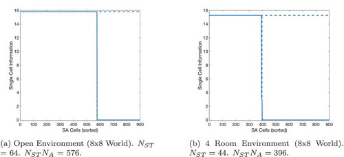
Figure 19 shows that these gating cells covered every valid¹⁴ combination of state cell and SA cell; in other words, that at least one gating cell fires uniquely for each valid combination of state and SA cell, and therefore that the gating layer is able to pass output from any SA cell to the action layer provided that they have the appropriate efferent connectivity to the action cells. Figure 20 indicates that this efferent connectivity has also self-organized; it shows that the appropriate number of gating cells have formed strong connections to one and only one action cell, allowing them to pass on activity to that cell and so produce action output as in Sec. 3.

Figure 19. The number of gating cells that encode each state-SA combination before and after training. Figure 19(a) shows that no gating cell fires uniquely for any combination of state and SA cells before the exploration period. Figure 19(b) shows that after training, gating cells fire uniquely for certain combinations of state and SA cells. Unlike the equivalent figure (Figure 13) in Sec. 4.1, which shows that at least one SA cell responds uniquely to every state-action combination after training, there is not a unique gating cell for every state and SA combination. This is because an SA cell (which encodes a unique combination of state and action) will only fire in conjunction with its associated state during exploration. Most state and SA cell combinations are therefore invalid: the cells in the gating layer will never experience this combination of inputs. We have therefore sorted the x-axis so that the valid state and SA cell combinations, which the agent can actually experience, lie along a diagonal, and we see that one gating cell has learned to respond to each of these valid combinations. Figure 19(c) zooms in on this diagonal (from Figure 19(b)) and shows that there are in fact several valid state-SA combinations for each state cell. This is because a number of SA cells exist for each state, each representing a different action in that state. We see that a gating cell fires uniquely for all of the state-SA combinations available for each state

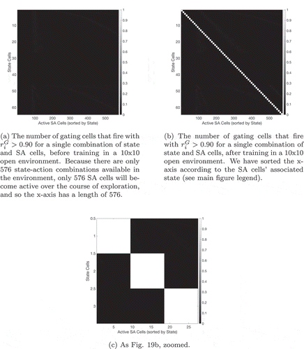
Figure 20. Efferent synaptic connectivity of gating cells after self-organization in an 8 × 8 open environment using the method described in Section 4.3. The x-axis shows the postsynaptic action cells, and the y-axis shows the presynaptic gating cells. For clarity, the y-axis has been sorted so that cells with a strong efferent connection to a particular action cell are grouped together. We see that the majority of gating cells (specifically $N_{ST}{N}_A$ = 576) form a strong synapse to one and only one action cell. This is what we expect: as in Figure 18(a) the maximum number of gating cells that can self-organize is 576, and these cells have also formed strong efferent connections to action cells, allowing them to pass on activity to the action cells and so produce action output as in Sec. 3

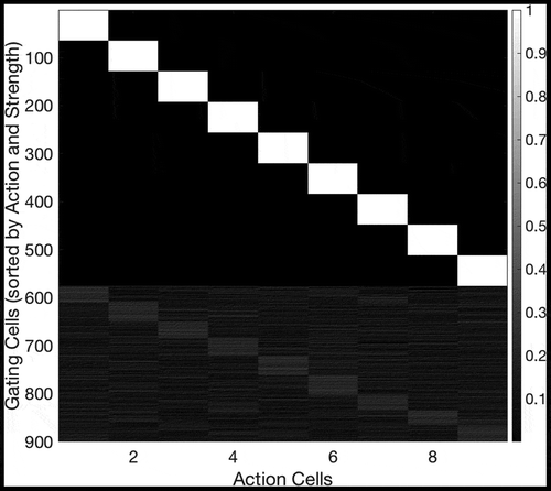
Figure 21 then explores the learned model’s ability to plan (according to the mechanisms in Sec. 3). This figure shows the percentage of correct navigation trials (navigating from one random state to a random goal state) that this model is able to achieve after exploring for a given number of timesteps during training. During training, the model uses the learning mechanisms described in this section as it explores the environment; during planning the model uses the planning mechanism described in Sec. 3. We see that the percentage of successful planning trials rises very quickly, even with relatively little training time. Figure 22 makes this clearer by showing the number of state-action combinations that the model experiences during learning. By comparing the percentage success rates in Figure 21 with the percentage of SA combinations experienced in Figure 22, we can see that the model’s ability to plan grows much faster than its experience of the environment. We also see that the model reaches 100% planning success long before it has experienced all SA combinations in the environment. In fact, only about 65% knowledge of the environment seems to be required for the model to navigate perfectly.

Figure 21. The percentage of successful trials if the model explores for a certain number of timesteps during training and is then used (instead of a hardwired model) to perform planning tasks identical to those in Section 3

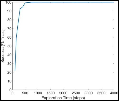
Figure 22. The percentage of SA combinations that the model has experienced after a certain number of timesteps. The model explores randomly, and so as its knowledge of the map grows more comprehensive, it becomes less likely to experience unknown SA combinations. The amount of environmental knowledge that the model contains therefore increases very quickly during early exploration but it takes many timesteps for the model’s knowledge of the environment to become comprehensive

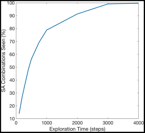
Discussion

Earlier we hypothesized that the similarity between gating cells and state-action cells meant that the mechanisms which self-organize SA cells could also self-organize gating cells. As described previously, the purpose of the gating cells is to pass activity from the SA cells to the action cells if and only if the SA activity is related to the agent’s current state. A gating cell should therefore receive activity from one SA cell and the state cell (or combination of state cells) that encode that SA cell’s preferred state, and should be able to propagate activity to that SA cell’s preferred action. Gating cells are under heavy inhibition such that they can only produce firing if they are receiving both SA and state input (see Equation 6(6) $r_i^G=\left\{\begin{array}{cc}{h}_i^G& h_i^G>t^G\\ 0& h_i^G\le t^G\end{array}\right.$(6) ), meaning that they only pass on activity from an SA cell when that SA cell matches the current state.

The results of this experiment demonstrate that the procedure described in Section 4.3.4 can fully self-organize the required connectivity between state cells, SA cells and gating cells (Figure 18). We also show that the resultant cells can be used to successfully plan solutions to grid world tasks (Figure 21). The number of gating cells increases relatively slowly but the ability to plan improves very quickly, demonstrating that relatively low SA and gating coverage is necessary for successful planning.

This section is the last of three experimental sections that are each devoted to methods of self-organizing an aspect of the model described in Section 3 as biologically plausibly as possible. Section 4.1 investigated mechanisms for self-organizing the afferent connectivity to SA cells. Section 4.2 investigated how the recurrent synapses between SA cells could learn to encode the causal transition structure of the environment in terms of states and actions. And finally Section 4.3 investigated mechanisms for self-organizing the afferent and efferent connectivity of the gating cells. In each section we have added the new mechanisms to the previous procedure, so that this section finally shows how each mechanism (SA self-organization, SA map learning, and gating cell self-organization) comes together to self-organize the main network used to perform planning tasks in Sec. 3. Section 5 will then cover the process of learning the sequences used by the hierarchical mechanism.

There remain certain biological implausibilities in this series of models. In particular, each of the three self-organization sections has required a longer list of activity propagation, inhibition and synaptic weight update events to happen in a precise order (algorithm 4). There is also the issue that the process described in algorithm 4 relies heavily on bandstop inhibition. However, bandstop inhibition is not a frequently used mechanism in modelling of this type and we cannot guarantee that it occurs in the brain.

Replication of a detour task

Having shown that the model can perform grid world tasks, we now demonstrate that it can replicate the characteristic performance of rats running a detour maze task. This task is still considered one of the key tasks demonstrating that cognitive maps exist (Simon and Daw 2011; Russek et al. 2016); work in humans strongly suggests an ability to solve detour tasks without re-learning, and these results have not yet been replicated by model-free or successor-representation based models (Russek et al. 2016; Fakhari et al. 2018).

The detour task was originally performed by Tolman and Honzig in the 1930’s, was re-performed by Alvernhe 2011 (Alvernhe et al. 2011) and used as a measure of model performance by Martinet 2011 (Martinet et al. 2011). Each version of this task has minor differences; this section replicates the version described by Martinet 2011 because it allows the fairest and most direct comparison between two neural network models of this task: the one proposed in this paper and Martinet 2011. We see it as a useful litmus test of the model’s basic ability to replicate map-based planning.

Planning with probabilistic propagation

Statement of problem

In the simulations described previously in this paper, the propagation of activation has been considered to be essentially deterministic. The predictable nature of activity propagation in these simulations means that the model tends to produce very similar paths if it re-encounters the same problem (the same agent and goal positions). This does not match the results from rats performing a detour task: Figure 26(a) shows that although rats tend to take the optimal path to a goal, they will take an alternative path in some trials. This suggested that our model’s planning mechanism was overly deterministic.

Furthermore, although most of the alternative models described in Sec. 2 do not consider transition probabilities,¹⁵ those models that do consider them are based on the principle of planning through decaying activation. In the paradigm of decaying activation, the passage of activation outwards from the goal produces the planning process. Activation decays as it propagates and so an optimal state-action or equivalent cell with receive a larger amount of activation compared to a less optimal cell, because the optimal state-action cell is connected to the source of activation (the goal) by fewer transitions and so receives activation that has decayed less. In this way the activation in these models becomes a crude approximation of the value-function that would be calculated by a model-based algorithmic planner (explicitly so in Friedrich et. al. 2016 (Friedrich and Lengyel 2016)). Decaying-activation models can account for transition probabilities quite easily by encoding them in the recurrent weights between SA cells (or their equivalents). Lowering the synaptic weight between two cells encodes that the corresponding transition is low probability and heavily reduces the amount of activity that propagates through this synapse. Essentially, low-probability transitions impart extra decay to activity passing through them, signalling their undesirability.

However, in the model that we have proposed in this paper (see Sec. 3), the wave-propagation planning mechanism relies exclusively on the timing of goal-based activity propagation through cells encoding the cognitive map, rather than how much activation those cells receive. The first SA cell to receive activation in each state represents the optimal action to take in each state, and the level of activation is not relevant. This planning mechanism has two primary advantages: it allows planning to become faster, and it removes the requirement for goal-based activation to decay, allowing the model to hypothetically cope with problems of much greater scale. It has an important disadvantage in that – because the precise activation of SA cells becomes irrelevant – the model cannot indicate transition probabilities by reducing the level of propagated activation to indicate a reduced transition probability. Increasing or decreasing the level of activation that an SA cell receives will not change the output of the proposed model, because it does not change whether that SA cell was the first cell to receive activation.

Hypothesis

We hypothesize that a timing-based planning model must instead indicate transition probabilities by altering the timing of activity propagation, and that this can be done either by delaying propagation or by making the probability of propagation dependent on the strength of the synapse, which in turn roughly indicates the transition probability (see previous section). Although this is a primarily practical decision, the nature of synaptic transmission makes this possible, even likely, especially if we expect planning to take place over a relatively short period of time.

This is because synaptic transmission is naturally unreliable (Maass 2014). Specifically, the spike of a presynaptic neuron does not reliably produce vesicle release. The probability of vesicle release (which depends on both the number of sites and the probability of release at individual sites) is affected by synaptic plasticity and makes up part of what is generally called synaptic weight (Abbott and Regehr 2004). The weaker the synaptic weight, the less likely that an action potential is to produce a postsynaptic spike at any given time. Furthermore, although cells connected by many tens of synaptic contacts show reliable responses to similar spike trains, cells that are connected by fewer synaptic contacts show much more variable responses because they are more reliant on the behaviour of individual synapses.

Modelling this process is not entirely straightforward as the stochastic propagation of this sort occurs on a short timescale whereas rate-coded models usually describe a longer period of time, averaging out individual spikes to produce activation values. However, we expect the planning process to take place over a relatively short timescale in order to produce useful behaviour (we explore the issue of planning speed at more length in Sections 3 and 6) and so we hypothesize that planning may occur using a stochastic propagation mechanism like the one we describe.

Task

An 8 × 8 grid world is bisected by a wall into two “rooms”. There are two points at which the agent may pass through the wall (Figure 9) called “gates”. The agent is placed in one room, equidistant from both gates, and the goal is placed in the other room, likewise equidistant. The number of trials in which the agent passed through each “gate” is recorded. The model may perform the task in one of two conditions.

Normal The model has learned the environment using the mechanisms described in the previous section, and performs the task “as is”. The recurrent SA to SA synapses that indicate the existence of transitions in the cognitive map are equal in weight, and all other recurrent synapses remain at zero.

Reduced The model is the same as in the “Normal” condition but the synapse representing the transition through the lower gate has been reduced to 10% of its original value.

Method

The network carries out planning as described in Sec. 3, with the single exception that the mechanism for propagating activity through the network has changed. In Sec. 3, SA cells are activated as follows:

(44) $h_i^{SA}=\sum _j{w}_{ij}^{GL-SA}{r}_j^{GL}+\sum _j{w}_{ij}^{SA-SA}{r}_j^{SA}$(44)

where ${\sum }_j{w}_{ij}^{GL-SA}{r}_j^{GL}$ is the summed input received from the goal cells and ${\sum }_j{w}_{ij}^{SA-SA}{r}_j^{SA}$ is the summed recurrent SA input.

In this experiment, in which we introduce probabilistic planning, SA activation is as follows:

(45) $h_i^{SA}=\sum _j{p}_{ij}^{GL-SA}{r}_j^{GL}+\sum _j{p}_{ij}^{SA-SA}{r}_j^{SA}$(45)

where $p_{ij}^{GL-SA}$ is stochastic, being either 1 or 0 depending on the value of $w_{ij}$ as follows:

(46) $\begin{array}{c}P\left(p_{ij}^{GL-SA}=1\right)=w_{ij}^{GL-SA}\\ P\left(p_{ij}^{GL-SA}=0\right)=\left(1-w_{ij}^{GL-SA}\right)\end{array}$(46)

As described in Sec. 4.2, the recurrent weights between SA cells are scaled such that:

(47) $\sum _j{w}_{ij}^{SA-SA}=4\mathrm{\forall }i$(47)

where ${\sum }_i{w}_{ij}^{SA-SA}$ is the sum of afferent weights received by postsynaptic cell $i$. In practice a cell will receive synapses from 9 cells (encoding 9 actions in its predicted successor state) so an individual synapse will usually have a value of 0.44 (4/9).

Results

Figure 23 shows that if the agent’s encoded cognitive map indicates (by way of reduced synaptic weights) that one path to a goal has a lower transition probability than another path, then the agent is much more likely to take the latter alternative path. In this experiment, the weight of the SA to SA synapses encoding the lower gate was reduced to 10% of their original value. We can see that in the normal condition (where the weights of the SA to SA synapses encoding both gates are equal) the agent ends up with an approximately equal chance of taking either gate. However, in the reduced condition, the agent has a much lower chance of taking the gate encoded by reduced SA to SA synaptic weights. In other words, if we reduce the weight of an SA to SA synapse to indicate a lower transition probability, the model is less likely to attempt that transition and more likely to prefer a more certain alternative route. The probabilistic propagation mechanism allows the model to incorporate transition probability into the planning process.

Figure 23. The probability that an agent will take the lower gate in the “normal” and “reduced” conditions, based on 100 trials in each condition. In the normal condition, the SA to SA weights encoding a transition through the lower gate (see Figure 9 for the structure of the two-gate environment) are kept at their original value of 0.44. The synaptic weights for both gates are therefore equal, and so the agent takes each path with approximately equal (50%) probability. In the reduced condition, the synaptic weights associated with the lower gate are reduced to 10% of their original value. Under the probabilistic planning paradigm described in Sec. 4.4, activation has a significantly lower probability of passing through the lower gate in any given timestep due to the reduced synaptic weights encoding this transition and therefore the agent is much less likely to pass through the lower gate. Note that the likelihood of taking either path depends on the ratio between the synapses encoding transitions through each gate and not on the absolute value of these synapses

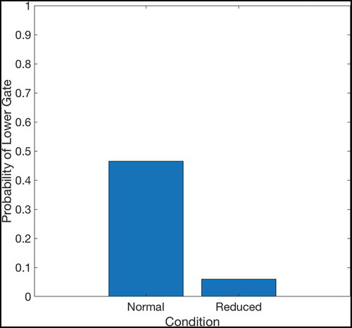
Discussion

The biological plausibility of the probabilistic planning mechanism is debatable, and largely depends on the timescale of the planning process because at longer timescales synaptic variability will simply translate into higher or lower firing rates. The probabilistic propagation mechanism makes much more sense if planning is considered to operate close to the level of individual spikes, similar to the model proposed by Ponulak 2013 (Ponulak and Hopfield 2013), but interpreted as a rate coded model.

If we assume that planning occurs on a relatively short timescale, say, 1 second, and that state-action cells fire at a rate between 5 and 50 Hz, and that most plans require activity to propagate through somewhere between five and twenty synaptic connections (more on this in Sec. 3) then it seems likely that the form of planning detailed here will rely on a relatively small number of spikes. If this is the case, then the probability of synaptic transmission between SA cells can genuinely affect the propagation of activation through the network and therefore a mechanism on the lines of that detailed in this section could exist and allow the network to plan in environment with probabilistic transitions.

Description of the detour task

The Tolman detour task (illustrated in Figure 24) is a maze with three paths of varying length: Path 1 (short), Path 2 (medium) and Path 3 (long). At the end of the maze is a food source (a goal state in the model). Put briefly, rats are allowed to explore the maze and are then expected to seek the reward. Path 1 is shortest; if it is open, rats will take it. If Path 1 is blocked at point A, so that only Path 2 and Path 3 are accessible, rats will then take Path 2 the majority of the time, without extensive retraining. If Path 1 is blocked at point B, rats take Path 3. This behaviour happens quickly, without extensive exploration, suggesting that rats are relying on a previously learned map of their environment to predict the outcomes of alternative trajectories through the environment.

Figure 24. The maze used in the Tolman & Honzig detour task, in which rats navigate through a maze to a food box (Martinet et al. 2011). The maze consists of three pathways (Path 1, Path 2 and Path 3) with different lengths. A block can be introduced at point A (preventing the rat from navigating through Path 1), or point B (preventing the rat from navigating through Path 1 or 2). A gate near the second intersection prevents rats from going right to left. This figure is reproduced from Martinet et. al. 2011 (Martinet et al. 2011) in accordance with the Creative Commons Attribution (CC BY) licence

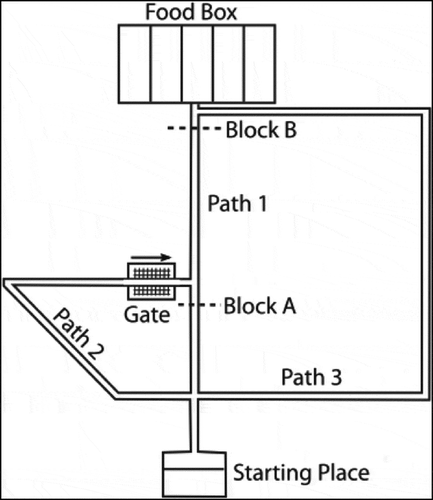
Detour task simulation procedure

A fully self-organizing version of the model (as formulated in Sec. 4) was trained using a protocol given in Martinet 2011, which was designed to emulate the protocol originally designed by Tolman and Honzig (Martinet et al. 2011). The training process took place over 14 simulated “days” and consisted of several different procedures. The model plans using probabilistic propagation (as described in Sec. 4.4). This was required to allow the network’s environment model to encode unexpected obstacles in a more realistic manner that includes some uncertainty about a newly encountered obstacle, rather than operating on the deterministic proposition that a transition is either possible or impossible, and so to allow the model to replicate the uncertainty and mistakes made by the experimental rats. Without this mechanism, the model simply takes the best path at all times. The probabilistic propagation mechanism is not therefore required to successfully complete the task, but is required to reproduce realistic results.

A consequence of representing transition probabilities using synaptic weights, and of the fact that the agent lacks any ability to probe a state without actually entering it, is that it is possible for the agent to believe that all three paths are blocked, and so refuse to enter any of them, thus not discovering that one of them is now open. To counteract this tendency, a stochastic exploration mechanism is used whereby if the agent has not moved for 200 timesteps the agent will then begin a short period of exploration (20 timesteps). A similar mechanism was used in Martinet 2011 (Martinet et al. 2011).

Day 1: A series of 3 “forced runs” were carried out. Each forced run consisted of a sequence of actions that the agent was forced to carry out. In other words, where the agent in Sec. 4 explored randomly, learning the SA cell responses, SA cell connectivity and gating cell connectivity as it went, the model now does the same for a pre-planned set of actions. Each forced run moved the agent from its start position along one path (P1 or P2 or P3) until the agent reached the goal; the three forced runs explored P1, P2 and P3 in succession. These forced runs were carried out by the network in Learning mode (see Section 4)

The forced runs were followed by nine trials in the open maze, where the model was switched into Planning mode (see Section 3) and all of the paths were unblocked. The end of the maze was set as a goal (see Figure 24) and the agent was allowed to navigate freely towards the goal. (Although these nine trials are identical and are not not strictly necessary in our formulation, we have kept the training procedure exactly as given in Martinet 2011 (Martinet et al. 2011).)

Days 2–14: On these days the model remained in Planning mode, although synapses were altered at unexpected obstacles. The model ran twelve trials every “day” for thirteen days, with the end of the maze set as a goal. In ten of these trials, Path 1 was blocked at point A. However, the entrances to Paths 2 and 3 were also blocked, forcing the agent to move to block A. Every time the agent encountered a block, the synapses making up the cognitive map were manually altered. This alters the cognitive map to include the block, and so alters the propagation of planning activity through the SA layer.

When the agent reached the block at point A, the entrances to Paths 2 and 3 were reopened so that the agent was free to choose either Path 2 or Path 3. The agent’s choice was recorded (see Figures 25 and 26). For each day, the 10 block A trials were randomly mixed with 2 non-successive runs with paths 2 and 3 blocked, to maintain the preference for Path 1. By non-successive, we mean that the agent never experienced 2 of these runs in a row.

Figure 25. Occupancy grids for Tolman & Honzig detour task. The occupancy grids show the probability that a modelled agent will at some point pass through each section of the maze during the various trial types. The scale runs from 0 to 1. An occupancy of 1 means that every agent passed through that point during every trial of that type; an occupancy of zero shows that no agent ever passed through that point in any trial of that type. We see that in the majority of Open trials, the agent takes the shortest possible route to the goal: the direct Path 1. In the majority of trials where Path 1 is blocked at Point A, the agent takes the now-shortest Path 2. Finally, in the majority of trials where Paths 1 and 2 are blocked at Point B, the agent takes the now-shortest Path 3. The qualitiative performance of both the Martinet model and the proposed model is similar

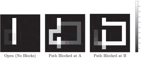
Figure 26. Comparison of model output to previous experimental and modelling results. Each box plot shows the distribution of route choices over trials of a particular type (Open, Blocked A or Blocked B). (a) shows experimental results from rats. (b) shows the results of the proposed model. The chosen path in each trial is recorded by measuring the last section of maze that the agent moves through before it reaches the goal

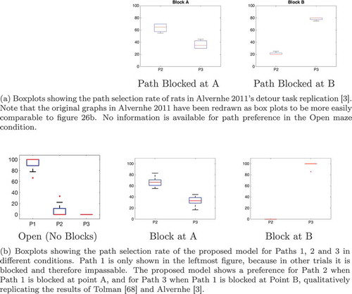
Day 15: Seven trials (in Planning mode) were run with a block placed at point B. As before, paths 2 and 3 were blocked until the agent reached point B, and then reopened. The agent therefore had a choice between choosing path 2, which was unsuitable given the block at point B, or choosing path 3. The results from both Alvernhe 2011 and Martinet 2011 (Martinet et al. 2011) showed that the agents reliably chose path 3, as did the proposed model. See Figures 25 and 26.

In summary, the protocol included three types of trials:

Open: In this condition, all of the paths are unblocked and the agent is allowed to navigate freely. This condition was present on Day 1.

Block A: In this condition a block was placed at point A, blocking Path 1 and forcing the agent to choose between Path 2 and Path 3. This condition was present on Days 2–14.

Block B: In this condition a block was placed at point B, blocking Path 1 and forcing the agent to choose between Path 2 and Path 3. However, in this condition the placement of the block renders Path 2 useless, so that the agent must use its knowledge of the environment to realize that Path 3 is the only way to reach the goal. This condition was present on Day 15.

As in Martinet 2011 (Martinet et al. 2011), 40 agents were simulated, and their results collated to produce the final analyses, shown in Figures 25 and 26.

Results of the detour task

Figures 25 and 26 demonstrate that the proposed model is capable of reproducing the behavioural results of Alvernhe 2011 (Alvernhe et al. 2011).

On Day 1, after exploring each of the three possible paths, the proposed model is allowed to navigate in the open maze (with no paths blocked) and shows a preference for Path 1, replicating the Path 1 preference seen in Martinet 2011 (Martinet et al. 2011). This is the shortest and most optimal route.

On Days 2–14, when the path is blocked at point A, the model chooses the shorter and more optimal Path 2 more frequently, whilst occasionally choosing Path 3, which is longer but also valid. When the path is blocked at point B on Day 15, the model reliably chooses Path 3, the only valid option.

Discussion

The behaviour of the model on the detour task replicates the essential finding of experimental and modelling literature: the agent reliably chooses shorter routes towards the goal. This result is intended to demonstrate that the model is able to replicate quantitative experimental results on one of the key model-based planning tasks. We have reused the detour task procedure described by Martinet 2011 (Martinet et al. 2011), which was taken from the original Tolman and Honzig paper (Tolman and Honzik 1930). The model proposed in this section differs from that proposed by Martinet 2011 in several significant ways.

Firstly, the model described by Martinet 2011 (Martinet et al. 2011) plans using the value of activation at different points in the map. Specifically, activity is injected into the map at the goal state and allowed to propagate through the map. As it propagates, the activity decays. This creates a gradient: the cell with the highest activation in each state represents the optimal action to take in that state. Unfortunately, the propagating activity eventually decays too much for SA cells to plausibly react to it, as described in Martinet 2011 (Martinet et al. 2011). The activity gradient can therefore only extend so far through the map, and in a complex map such as a maze this activity may decay very quickly. Martinet introduces a variable-resolution mapping mechanism that can extend this range, but this mechanism requires that the environment is composed primarily of long straight-line segments connected by sharp discontinuities, a condition that is true of the detour maze task but does not extend well to other environment types. See Sec. 2 for more details.

In constrast, the proposed model does not require an activation gradient. In the proposed model, the optimal SA cell for each state receives activity first, and so the first SA cell to receive activation in each state inherently represents the optimal action to take in that state. The level of activation is not relevant. This means that the activity does not need to decay, and so we do not experience the dropoff problem described in Martinet 2011 (Martinet et al. 2011). The planning mechanism is therefore more extensible to different map types and sizes, and also allows us to introduce a flexible hierarchical system for improving the efficiency of planning (see Sec. 3 and 5).

The proposed model and Martinet 2011 (Martinet et al. 2011) also differ in how they adapt to dynamically changing environments. Martinet 2011 manually identify cells whose synapses must be adjusted to encode a new obstacle and then hardwire the synapses between these cells to encode this information. To be specific, they set the relevant synaptic weight to 0.9 if the agent experiences a successful state transition, and halve the weight if the agent experiences a failed transition. We used a similar mechanism to obtain the detour task results that we have show in Figures 25 and 26, but the Hebbian mechanisms for learning state transitions during initial training (see Sec. 4) are equally able to adjust the cognitive map to reflect later changes in the environment.

Having described both the learning and planning mechanisms of the proposed model, and tested it on a canonical behavioural task, the next sections (3 and 5) will discuss the extension of this model to a formulation that encompasses hierarchical behaviour.

Encoding useful behavioural sequences by self-organizing a layer of sequence cells

Statement of problem

The work described in Section 3 demonstrated that sequence cells (Figure 1) can be used to improve the efficiency of the network’s planning. The planning process requires a wave of activity to travel from the SA cells representing the goal state to the SA cells representing the agent’s current location. Sequence cells assist this process by acting as a “shortcut” for the wave, allowing it to travel faster through frequently experienced areas of the state-action space. To do this, the sequence cells require a particular pattern of connectivity with and from the SA cells.

We wish to explain how the model could self-organize such connectivity. Furthermore, since the number of possible trajectories that the agent may take is very large, including many that are not helpful in the majority of tasks, the sequence cells should learn to encode the most behaviourally-useful sequences that the agent has experienced: sequences that move the agent directly between important states such as bottlenecked areas of the environment. How should the sequence cells identify and encode these sequences as the agent performs tasks?

Hypothesis

We hypothesize that the connectivity between sequence cells and SA cells comes about through a form of trace learning, similar to that seen in Sec. 4.2. As discussed in that section, the trace learning rule is a variant of Hebbian learning that ties together cells which fire close together in time. In this case a sequence cell that has been stimulated by an SA cell will remain in an active learning state for several more state-action combinations, therefore building up afferent and efferent connectivity to a sequence of SA combination cells.

The most behaviourally relevant sequences are those which provide a direct path through an important area of state-action space and so provide maximum augmentation to the network’s ability. We hypothesize that such sequences are likely to be encountered more frequently than other sequences¹⁶ when moving purposefully through the state space under the kinds of route planning mechanisms demonstrated in this paper. Specifically, the basic route planning mechanisms described earlier in this paper tend to move the agent along a direct route from its current state to a goal state. If sequence cells are incorporated into the network, then these cells can learn these direct routes through the state space that emerge from the basic planning mechanism.

In this way, the basic planning mechanism (which generates direct routes between states) operates in tandem with the hierarchical model extension incorporating sequence cells (which learn these useful direct routes). The final model formulation presented in this section therefore offers a biologically plausible solution to how hierarchical behaviour can self-organize in the brain through unsupervised learning.

The requirement for humans to accumulate extensive task experience to achieve a high level of automaticity supports this hypothesis, as does the fact that it seems to be necessary for learners to spend disproportionate amounts of time on aspects of a task that they find difficult if they wish to further improve their skills. To mimic this process, we decided to take the grid world navigation tasks that we had used to test the model in Section 3 and now use them to train the model.

Task

The task is fundamentally similar to the grid world navigation task described by Section 3. The agent is placed at a random position in one of four grid worlds. Two of these worlds are the small (8x8) open and maze worlds depicted by Figure 5. The other two worlds are the same but scaled by ^~2:1, so that they are 18 × 18. The agent can move one space at a time in eight compass directions¹⁷ or stay still, giving nine possible actions.

A random state is designated as the goal and the agent is required to navigate to this state to complete the task. If the agent reaches the goal location then the task has been been completed successfully. If the agent fails to reach the goal location within 1000 timesteps then the agent has failed the task. At the same time, the agent is both learning and using sequences of actions by altering the connectivity between the sequence cell layer and the SA cell layer (see below).

Network model

Algorithm 5 Learning Sequences During Planning. This describes the network’s operations during one step in the planning process, based on alg. 1. The steps that have been added in this version are emphasized with italics. Steps in (brackets) only occur if there is activity in the action cell layer signifying that an action has been selected for the agent’s current state. All plasticity is Hebbian unless otherwise specified.

Cell Firing State Cells & Goal Cells Fire (one-hot)

Activity Propagation SA Cells & Goal Cells to SA Cells (3)

Inhibition SA Cells: Rescale SA Activity in All Active States (4)

Activity Propagation State Cells & SA Cells to Gating Cells 5)

Inhibition Gating Cells: Threshold ((6))

Activity Propagation Gating Cells to Action Cells (7)

Inhibition Action Cells: Winner-Take-All (8)

(Agent) Agent Moves to Successor State

(Activity Propagation) State Cells, Action Cells and SA Cells to SA Cells (49)

(Inhibition) SA Cells: Winner-Take-All (50)

(Activity Propagation) SA Cells to Sequence Cells (1)

(Inhibition) Sequence Cells: Winner-Take-All (51)

(Synaptic Plasticity) Set Memory Trace: Sequence Cells (52)

(Synaptic Plasticity) Set Memory Trace: SA Cells (52)

(Synaptic Plasticity) Trace Learning: Sequence Cells to SA Cells (53)

(Synaptic Plasticity) Trace Learning: SA Cells to Sequence Cells (54)

(Synaptic Plasticity) Trace Learning: Synaptic weights rescaled (55) and (57)

(Reset) All Cells Reset to Zero Activation

The network architecture

The network used in this experiment has the same structure as that used in the Section 3 (Figure 1). It is assumed that basic environmental learning has already taken place, i.e. that the agent has already explored its environment and that the self-organization of SA cell responses, recurrent SA connectivity and gating cell connectivity has already occurred as in Section 4. For the purposes of this experiment, only the connectivity between the sequence cell layer and the SA cell layer is considered to be plastic.

As stated previously, the bi-directional connectivity between the sequence cells and SA cells is learned during the performance of planning tasks, where the network is exploiting a previously learned causal model in the recurrent connections between SA cells. In the simulations that follow, during the training phase in which the connections between the SA cells and sequence cells self-organize, the sequence cells are not actually allowed to influence the planning mechanism as goal-related activity propagates through the SA layer. This simplification of the training phase is designed to demonstrate how the development of sequence cells encoding a motor hierarchy can be driven by route planning using just the causal model previously learned in the recurrent connections within the SA layer. However, during this training phase, the connections between the sequence cells and SA cells are updated using trace learning rules incoroporating a trace whenever the agent takes an action. This allows the sequence cells to learn to encode the most frequently used state-action sequences over time. As with gating cells, the layer of sequence cells operates as a competitive layer during learning, with individual sequence cells inhibiting each other. This has the effect that individual sequence cells compete to learn to represent particular state-action sequences, within different cells learning different sequences. After this training phase has self-organized the bi-directional connections between the SA cells and sequence cells, the sequence cells are then allowed to influence activity within the SA layer during subsequent testing of the effects of sequence cells on route planning and movement through the environment.

Route planning – a timestep where no action is taken

The state cells fire, encoding the current state using a one-hot encoding. At the same time, the goal cells fire, encoding the location of the goal. The SA cells are then updated by activity from the goal cells and from other SA cells according to the following equation:

(48) $h_i^{SA}=\sum _j{w}_{ij}^{GL-SA}{r}_j^{GL}+\sum _j{w}_{ij}^{SA-SA}{r}_j^{SA}$(48)

where ${\sum }_j{w}_{ij}^{GL-SA}{r}_j^{GL}$ is the input received from the goal cells, and ${\sum }_j{w}_{ij}^{SA-SA}{r}_j^{SA}$ is the recurrent SA input. (The SA layer does not receive activation from the state cells – this occurs only during learning for the purpose of self-organizing the state-action responses and consequently the cognitive map.) SA cells experience divisive inhibition, rescaling the activity of SA columns so that each currently active column is rescaled to sum to 1, and each inactive column remains inactive (with a sum of 0) as shown in Equation (4)(4) $\sum _i{r}_i^{SA}=\left\{\begin{array}{cc}1& {\sum }_i{h}_i^{SA}>0\\ 0& {\sum }_i{h}_i^{SA}=0\end{array}\right.$(4) .

The effect of this recurrent SA stimulation combined with firing from the goal cells is to create a propagating wave of activity spreading through the SA layer. The wavefront of this activity spreads a little further every timestep.

After the SA cells have been updated, they propagate activity to the gating cells (Equation 6(6) $r_i^G=\left\{\begin{array}{cc}{h}_i^G& h_i^G>t^G\\ 0& h_i^G\le t^G\end{array}\right.$(6) ). The gating cells are under heavy inhibition such that they can only produce firing if they are receiving both SA and state input (Equation 6(6) $r_i^G=\left\{\begin{array}{cc}{h}_i^G& h_i^G>t^G\\ 0& h_i^G\le t^G\end{array}\right.$(6) ). Activity propagates from the gating cells to the action cells (Equation 7(7) $h_i^A=\sum _j{w}_{ij}^{G-A}{r}_j^G$(7) ). If no gating cell fires, then no action cell will fire; in this case no action will be taken at that moment and the wave will continue to propagate, allowing SA activation to spread further through the layer. However, if any action cell becomes active, then the set of events described in the rest of this simulation produce (below) will take place. These events are bracketed in algorithm 5.

Learning hierarchy of action sequences – if an action is taken

The agent takes an action, and updates the world.

The SA layer receives a combination of sensory and motor inputs (as well as input from the recurrent synapses $w_{ij}^{SA-SA}$) that reflect the state-action combination chosen by the planning mechanism as follows:

(49) $h_i^{SA}=\sum _j{w}_{ij}^{S-SA}{r}_j^S+\sum _j{w}_{ij}^{A-SA}{r}_j^A+\sum _j{w}_{ij}^{SA-SA}{r}_j^{SA}$(49)

where $h_i^{SA}$ is the activation of a state-action cell, ${\sum }_j{w}_{ij}^{S-SA}{r}_j^S$ is input from state cell $j$ weighted by the incoming synapse, ${\sum }_j{w}_{ij}^{A-SA}{r}_j^A$ is the equivalent input from action cell $j$ and ${\sum }_j{w}_{ij}^{SA-SA}{r}_j^{SA}$ is the recurrent SA input. This combination of inputs strongly activates the specific SA cell that represents the correct combination of state and action. WTA competition is then applied as follows:

(50) $r_i^{SA}=\left\{\begin{array}{cc}{h}_i^{SA}& h_i^{SA}={max}_i\left\{h_i^{SA}\right\}\\ 0& h_i^{SA}<{max}_i\left\{h_i^{SA}\right\}\end{array}\right.$(50)

where ${max}_i\left\{h_i^{SA}\right\}$ is the activation value of the most active cell in the SA layer. This leaves only one SA cell active: the SA cell representing the state-action combination that the agent is currently experiencing.

The activity from this SA cell feeds into the sequence cell layer (Equation 1(1) $h_i^{SQ}=\sum _j{w}_{ij}^{SA-SQ}{r}_j^{SA}$(1) ). WTA competition is then applied to the sequence cells as follows:

(51) $r_i^{SQ}=\left\{\begin{array}{cc}{h}_i^{SQ}& h_i^{SQ}={max}_i\left\{h_i^{SQ}\right\}\\ 0& h_i^{SA}<{max}_i\left\{h_i^{SQ}\right\}\end{array}\right.$(51)

where ${max}_i\left\{h_i^{SQ}\right\}$ is the activation value of the most active cell in the sequence cell layer.

A trace rule is used to alter the connectivity between the SA layer and the sequence cell layer (in both directions). The trace rule is similar to those described in Sec. 4.2 (Equation 23(23) $\mathrm{\Delta }{w}_{ij}^{SA-SA}=k^{TR}{\bar{r}}_i^{SA}{r}_j^{SA}$(23) ) but uses a more complex trace value, which is calculated at this point in the timestep as follows:

(52) ${{\bar{r}}_i}^t=r_i^t(1-\eta )+{\bar{r}}_i^{t-1}\eta$(52)

where $r_i^t$ is the current firing rate of a sequence or SA cell $i$ at time $t$, ${{\bar{r}}_i}^t$ is the memory trace value of $r_i$ at time $t$, ${\bar{r}}_i^{t-1}$ is the memory trace value of $r_i$ at time $t-1$, and $\eta \in \left[0,1\right]$ is a constant that determines how much the current trace value reflects past firing rates as opposed to present firing rates. This trace value varies from that used in Sec. 4.2, which only considered cell firing one timestep in the past. In Sec. 4.2 only one timestep of information is necessary to encode a transition from one state to another. By contrast, in this section we are interested in forming sequence cells that will learn to associate a sequence of SA cells over a period of several timesteps. A slowly fading memory trace is therefore required, where the parameter $\eta$ effectively determines the decay rate. Note that both forms of trace rule are purely local, relying only on the activities of the pre- and post-synaptic neurons. As such, these learning rules can be considered relatively biologically plausible. The effect of trace learning is to connect cells that fire over a period of time.

The synapses between SA cells and sequence cells are then updated according to a trace rule as follows:

(53) $\mathrm{\Delta }{w}_{ij}^{SQ-SA}=k^{SQ-SA}{\bar{r}}_j^{SQ}{\bar{r}}_i^{SA}$(53)

(54) $\mathrm{\Delta }{w}_{ij}^{SA-SQ}=k^{SA-SQ}{\bar{r}}_j^{SA}{\bar{r}}_i^{SQ}$(54)

where ${\bar{r}}_i^{SQ}$ and ${\bar{r}}_j^{SQ}$ are the trace values of sequence cells $i$ and $j$ respectively, ${\bar{r}}_i^{SA}$ and ${\bar{r}}_j^{SA}$ are the trace values of SA cells $i$ and $j$ respectively, and $k$ is a constant denoting learning rate. Note that $k^{SA-SQ}$ is considerably larger than $k^{SQ-SA}$. This is necessary because it means that the last SA cell to fire in a sequence will have an extremely strong weight to the sequence cell. This brings about the characteristic sequence cell connectivity described in Sec. 3, where the sequence cell receives strong inputs from the last SA cell in the sequence (and therefore the first to receive activation from the propagating wavefront, which propagates from the goal) whereas all of the SA cells in the sequence receive relatively similar activity from the sequence cell. This is further effected by the rescaling mechanism, which ensures that:

(55) $\sum _j{w}_{ij}^{SA-SQ}=1\mathrm{\forall }i$(55)

and any synaptic weights that are too low are reduced to zero:

(56) $w_{ij}^{SA-SQ}=\left\{\begin{array}{cc}{w}_{ij}& w_{ij}\ge t^{SA-SQ}\\ 0& w_{ij}<t^{SA-SQ}\end{array}\right.$(56)

where $t^{SA-SQ}$ is a threshold constant.

$w_{ij}^{SQ-SA}$ are rescaled so that

(57) $\sum _i{w}_{ij}^{SQ-SA}=1\mathrm{\forall }j$(57)

Note that the rescaling is performed with reference to the sequence cells in both Equations 55(55) $\sum _j{w}_{ij}^{SA-SQ}=1\mathrm{\forall }i$(55) and 57(57) $\sum _i{w}_{ij}^{SQ-SA}=1\mathrm{\forall }j$(57) . This is because each sequence cell is intended to represent a single sequence, and so the amount of afferent connectivity that each sequence cell receives, as well as the amount of efferent connectivity, must be regulated. By contrast, a given SA cell may be part of many sequences or none.

Finally, the activity of all cells is reset. Parameters are given in Table 5.

Table 5. Table of parameters for the learning of sequence cells as described in Section 5

Parameter	Value
Trace Constant Eta $\eta$	0.5
Sequence Cells to SA Cells Learning Rate ($k^{SQ-SA}$)	11
SA Cells to Sequence Cells Learning Rate ($k^{SA-SQ}$)	${10}^{26}$
SA Cells to Sequence Cells Threshold ($t^{SA-SQ}$)	$0.1$

Results

Figure 27 shows some examples of the sequence connectivity that self-organizes using this method. We see that these learned sequences are composed of a set of state-action combinations that describe a reasonably logical journey from one area of the map to the other. The learned sequences have a single “entry” point at the beginning of a sequence and a single “exit” point at the end of this sequence. This contrasts with an approach that might produce multiple entry points and multiple exit points (see for example (Pickett and Barto 2002; Botvinick et al. 2009)). The weight structure is consistent with that described in Section 3, with sequence cells receiving synapses only from the last SA cell in a sequence and sending synapses to all SA cells in that sequence.

Figure 27. Examples of two learned sequences. The magnitude of each arrow represents the weight of the synapse from the sequence cell to that SA cell (left column) or the weight of the synapse to the sequence cell from that SA cell (right column). Synapses have been normalized so that 1 is the maximum synapse. We see that the weight structure is consistent with that described in Section 3, with sequence cells receiving synapses only from the last SA cell in a sequence (b, d) and sending synapses to all SA cells in that sequence (a, c). See Figure 3(b) for legend

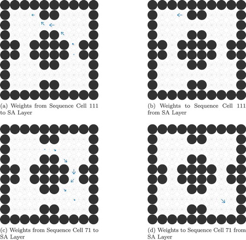
Figure 28 shows the results of a set of planning experiments using sequences learned in the manner described in this section. These tasks were conducted as standard planning tasks: the agent was placed in the 8 × 8 open environment and the 8 × 8 4-room environment (Figure 5). In each trial a random location within this grid is designated as the agent’s goal and another random location is designated as the agent’s starting point. The agent can move one space at a time in eight compass directions¹⁸ or stay still, giving nine possible actions. The task is for the simulated agent to navigate to the goal location. If the agent reaches the goal location then the task has been been completed successfully. If the agent fails to reach the goal location within 100 timesteps then the agent has failed the task. Figure 28 shows that under these conditions the model is able to achieve 100% success rates in both the 8 × 8 open environment and the 8 × 8 4-room environment.

Figure 28. Success rates in planning task when using learned sequences. This figure shows the percentage success rates of the network in 100 trials

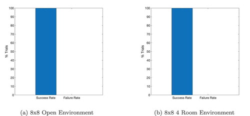
Figure 29 shows that states that are occupied more often have more associated sequences. To obtain this figure we count the number of sequences associated with each state by counting the number of synapses that each SA cell receives and then associating them with the state which that SA cell represents. The results strongly suggest that the model tends to learn sequences that are “useful”, in other words sequences that occur frequently in the solutions to planning tasks that take place in this environment. We also see that, at least in the relatively small 8 × 8 environment, most states are associated with at least one sequence, suggesting that the learned sequences cover the environment reasonably well and so may be useful even in less commonly used areas of the state space.

Figure 29. The occupation of different states during the sequence-learning period. (a) shows the probability of an agent occupying any given state in this 4-room environment (Figure 5) while (b) shows the number of sequences associated with each state after 300 planning tasks in this environment. By comparing the two, we see that states that are occupied more often have more associated sequences. This strongly suggests that the model tends to learn sequences that are “useful”, in other words sequences that occur frequently in the solutions to planning tasks that take place in this environment

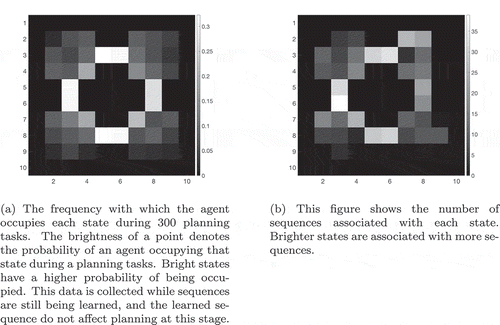
Discussion

In Section 3 we demonstrated that the network can use a layer of sequence cells to assist planning, reducing the time it takes for activity to propagate through the SA layer and so reducing the amount of planning time required to reach decisions. There remained, however, the question of how the agent should produce the required connectivity between the sequence cells and SA layer, thus learning useful state-action sequences.

In this section we have demonstrated that the network is able to successfully learn state-action sequences which cover the commonly used area of the state-action space. Because the learned state-action sequences tend to be those that occur most frequently during the performance of navigation tasks (Figure 29) they are in the main appropriate for the structure of the environment (e.g. moving from one room to another in a four-room maze). The learning procedure described in this section requires that trace learning takes place at specific times in each timestep, when the SA cells are representing the appropriate information about combinations of state and action. We hypothesize that the firing of the action cells once planning is complete and the next action has been decided, and the flood of sensory and motor feedback produced by the performance of that action, strongly activate the SA cell representing the current state and action, allowing sequence cells to connect to that SA cell.

The question then arises of why the sequence cells only form synapses to the SA layer at this point in the timestep. It is possible that SA cells fire very strongly at this point, boosted by sensory and motor feedback, while the level of SA activity during the planning process is much weaker. Equally, it is possible that plasticity is gated in some fashion such that the synapses are only plastic at this point in the timestep.

Replication of human planning times

As humans spend more time in an environment, they will learn a cognitive map but will also begin to learn useful sequences of actions for performing tasks in that environment. In wayfinding experiments, this means that as humans perform more navigation tasks in an environment,¹⁹ they should show faster decision times at choice points. This prediction is difficult to validate, because very few papers on human navigation give planning times and none describe how planning time changes with experience. However, there is circumstantial evidence which supports this account.

In particular, Howard 2014 (Howard et al. 2014) found that the decision-making time of humans doing a wayfinding task in a virtual reality replication of the London borough of Soho was proportional to the absolute path length between the current choice point and the goal. The correlation was strongly significant, and of medium strength (correlation constant = 0.363; p < .01). Although the proposed model reproduces this correlation between planning time and path length, in its base state without sequence cells the proposed model gives a much stronger correlation (correlation constant = 0.88) than is shown in the Howard 2014 data. Introducing the hierarchical mechanism (utilizing sequence cells) decreases planning time and introduces more variation, giving results (correlation constant = 0.69) that are closer to Howard 2014’s data. As environments become larger, and the available repertoire of learned sequences becomes larger and more complex, we believe that the effect of the hierarchical mechanism on planning time would be even stronger, and so potentially produce planning-time vs. path length correlations close to those found by Howard et. al. 2014.

Discussion

Aim 1: Learn and use a causal cognitive map

After considerable study over the last few years, the production of a cognitive map and the use of it for consequent/concurrent model-based planning seems to be a necessary element for the production of some behaviours (see Sec. 1). Such maps appear to be particularly important in the context of revaluation and contingency-change tasks Russek2016,Fakhari2018.

Given the apparent importance of this mechanism, one of the primary aims of this work was to investigate this process in the context of a (biologically plausible) neural network and there are two fundamental elements that therefore had to be replicated: the ability to learn a causal model of the simulated agent’s environment, and the ability to use this model to generate behaviour. The other aims of this work – to remain broadly consistent with known neurobiology, to address outstanding questions raised by previous models of this mechanism and to extend this mechanism to include hierarchical mechanisms – rest on the prerequisite that the model is ultimately able to produce the desired behaviour, or at least represents a meaningful step towards such a model.

Progress made by this paper

The model described in this paper had to replicate two primary elements of model-based planning: the production of a cognitive map and the use of this map to produce behaviour. In the process of doing so, we attempted to address the limitations of the decaying-activation theory (in particular, its inability to solve problems of arbitrary length) by using an alternative planning mechanism.

Section 3 demonstrated that a particular network architecture was capable of producing solutions to grid world tasks, so long as the model was provided with a valid cognitive map that described the state transitions that were possible in each grid world. An advance of the work in this paper has been to give a full account of how a propagating wavefront mechanism would work as the basis for planning using a cognitive map. The reason for doing so is that such a mechanism is more efficient, more robust and more powerful than the decaying-activation mechanism used by previous models.

As described in Sec. 3, a propagating wavefront mechanism fundamentally relies on the timing of goal-based activity propagation through the cognitive map, rather than how much activity different cells receive. Rather than hypothesizing that activity decays as it propagates (which leads to the aforementioned problem that this activity may eventually decay to nothing) we hypothesize that activity propagates along the shortest path to the goal fastest. In other words, we hypothesize that optimal actions are driven by the timing of activation rather than the level of activation. The first SA cell to receive activation in each state is considered the optimal action to take in each state, and its level of activation is not relevant. This mechanism owes inspiration to work by Ponulak & Hopfield 2013 (Ponulak and Hopfield 2013). Their paper described a model in which a wave of activity propagates through a 2D layer of topologically organized pure state cells (neighbouring state cells were recurrently connected) and showed that this wave carried information about the direction of the goal. Specifically, if the goal is east of a state cell, the wavefront will “hit” the state cell from that direction. Ponulak showed that an anti-STDP mechanism could record this information in the recurrent synaptic connectivity of the layer by strengthening the synapses between cells to indicate the direction from which they were “hit” by the wave.

The mechanism that we have proposed retains the insight that the propagation of a wavefront can carry information about the direction of a goal, but uses this information in a rather different way. Rather than use a propagating wavefront to adjust the synapses between pure state cells and thus produce a synaptic vector field, we have proposed that a propagating wavefront can identify and output the most valuable state-action combination for a given state. The proposed mechanism is therefore able to improve on the mechanism described by Ponulak & Hopfield in several key ways. Firstly, because the proposed planning mechanism is able to work in a state-action map, it is able to output explicit actions that move the agent towards the goal (see below). Secondly, because the proposed planning mechanism is able to perform planning without requiring a period of synaptic plasticity, it seems likely that an agent using this mechanism would be able to plan more quickly, and would not have to “undo” the new synaptic weights if there is a change in the goal state or the transition structure of the environment. Thirdly, because the proposed planning mechanism is able to plan without altering the synaptic weights that encode the cognitive map, we can store information in these weights, such as transition probabilities. Finally, the proposed planning mechanism is able to interface with a hierarchical behaviour mechanism.

The proposed propagating wavefront mechanism will produce a suggested action as soon as the propagating goal-based activity reaches the agent’s current state, and it is therefore the fastest way of producing an action using propagating activity. It is, after all, impossible to read the value of decaying activation at the agent’s current state until the neurons representing actions at that state become active. And the gating mechanism that we describe provides a way of ensuring that the first active neuron in the current state is detected and the appropriate action read out. By contrast, Cuperlier 2007 (Cuperlier et al. 2007) reads out an action only when the activity in the network is considered “stable”, which presumably requires a significant further period of stabilization; Hasselmo 2005 (Hasselmo 2005) waits for a specific period of time before reading out an action and thereby risks reading out too early (before activity has reached the right part of the map) or too late (when the situation has changed or time has been wasted).

Mechanistic efficiency does not, of course, mean that the theory is true, and thoughts on testing the contrasting predictions made by decaying-activation theory and the propagating wavefront theory based on timing are given in the next section (6.1). However, the prediction made by the propagating wavefront mechanism that planning times will be dependent on the distance of the goal can potentially by used to compare it with other theories.

The propagating wavefront mechanism also seems likely to be more robust to noise. The decaying-activation method relies on comparing the precise value of activation over different states or state-actions, and if noise alters these values a decaying-activation mechanism may therefore produce maladaptive results. By contrast, the precise effect of noise on a propagating wavefront model is likely to depend on how it interacts with inhibitory mechanisms.

Finally, the propagating wavefront mechanism is able to perform longer and more complex tasks than a decaying-activation mechanism. The level of activity in cells is not relevant, and the activity is not required to decay, so the level of activity can be kept high and the propagation of activity can continue indefinitely.

As stated previously, we intended to give a full explanation of how planning with propagating wavefronts could work. To do this, we needed to show not only how the actual propagation would occur, but also to explore the mechanisms that would be needed to support it. In particular, the use of a propagating wavefront mechanism adds new complexity to the problem of how to read out actions from the planning mechanism, and how to plan when the transition structure of the environment is not deterministic. We have therefore introduced a probabilistic propagation mechanism (Section 4.4) in order to incorporate transition probabilities into the planning process, and used a layer of gating cells under heavy inhibition to output actions from the planning mechanism.

Predictions and falsification

The model that we have proposed predicts that certain tasks can be solved by model-based planning mechanisms, implemented by a specific set of neural mechanisms. By studying the model, we can elaborate on this prediction, highlighting areas in which this model can be compared to other models and to experimental data, and therefore in which aspects of the model can be improved or discarded.

One way that this model, or a more advanced version of this model, could be falsified is if further inquiry into the mechanism of model-based planning falsifies the idea that planning results from the propagation of activity through some form of map representation. An alternative planning hypothesis, not based on propagation, is that task solutions are calculated by some sort of heuristic. For example, there are models of spatial planning that suppose that planning is done by triangulating the direction of the goal and then moving in that direction, without planning an explicit path through the environment (Burgess et al. 1994). However, this does not seem to fit the available evidence given by planning times: work on street navigation (Howard et al. 2014) and the Tower of London task (Ward and Allport 1997; Cazalis et al. 2003) suggest that planning times are proportional to the length of solution, which suggests that the planning process involves trying to produce a solution rather than merely a direction of travel through state space.

Another way that the backward (goal-based) propagation mechanism could be (partially) falsified is if it were demonstrated that map-based planning activity propagates forwards from the agent to various goal locations. The evidence conflicts on this point. The findings of Kurth-Nelson et al. (Kurth-Nelson et al. 2016) indicate that retrieval of state transition sequences occurs in a backwards direction (Kurth-Nelson et al. 2016). In contrast, the findings of Johnson et. al. 2007 show that sequences of states travel forward from a rat’s position to investigate different potential paths when deciding which branch of a T-maze to search for food (Johnson and Redish 2007). Finally, the verbal reports of London taxicab drivers indicate that an important mechanism for wayfinding is to identify the compass direction of the goal and then plan a short distance of actions forwards from their current state that will take them in the correct direction (Spiers and Maguire 2008). We are not aware of robust map-based network models which plan using a forward mechanism and other modellers have criticized the idea of planning based on forward sweeps through a synaptic map (Chersi and Pezzulo 2012). It is, however, entirely possible that forward and backward propagation coexist in the brain, either as cooperating parts of a planning mechanism or as epiphenomena reflecting other processes.

The model predicts, unlike other models, that the timing of the activation propagation is important to the planning process and that the relative activation of cells is largely irrelevant. Implementing a decaying activation planning paradigm either requires neurons to be able to distinguish very similar firing rates (because the local gradient is usually very small) or is only able to plan over a very limited number of consecutive actions before the activity decays to noise level. If it is not possible for neurons to detect fine differences in firing rates then the prevailing paradigm of planning by decaying activation becomes less credible.

In this light, it is perhaps important to bear in mind that neurons exhibit substantial trial-to-trial variability that seems to be linked to intrinsic factors such as synapse unreliability and synaptic background noise (Faisal et al. 2008; Maass 2014). Even if a presynaptic cell is driven repeatedly with identical stimuli, there is trial-to-trial variability in the postsynaptic response (Faisal et al. 2008). This variability primarily affects the membrane voltage and consequently the production of individual action potentials, but it suggests that it would be difficult for a neural system to reliably set up and maintain a large-scale decaying-activation gradient in which small variations in relative firing rates carry crucial information. Furthermore, patch-clamp experiments by London et. al. 2010 (London et al. 2010) found that small variations in firing rate (a perturbation consisting of a single extra spike in one neuron) produced approximately 28 additional spikes in that neuron’s postsynaptic targets. This again suggests that it would be difficult to reliably set up a large-scale fine-grained activation gradient, although it also suggests that small differences in relative firing rates could be plausibly amplified and read out.

Another way to falsify the propagating wavefront hypothesis is to investigate whether the planning process takes the same time regardless of the number of steps involved. If this is so, then it suggests that the timing of neuron activation does not depend on the task, and so that the timing of different neurons does not affect the planning process. As we argued earlier in this section, available experimental evidence seems to indicate that planning time is at least partly proportional to the number of the number of steps to the solution of the task (Ward and Allport 1997; Cazalis et al. 2003; Howard et al. 2014).

Further work

Further modelling work is required to discover whether the current limitations of the model that we propose are inherent in the mechanisms that we are using or whether they can be improved. Further experimental work is also required, to test the predictions of this model with of other models where they conflict, and thus to determine which theories more accurately represent the planning mechanisms in human and animal brains.

Obviously, both the model-based and the model-free formulations of reinforcement learning are extremely active research topics at present. There is also a field investigating how these paradigms might compete and cooperate in the production of behaviour (Keramati et al. 2011; Dolan and Dayan 2013; Nagabandi et al. 2017; Chebotar et al. 2017). Further research will make it clearer what tasks are and are not solvable with each of these approaches, and how they might need to be combined. With reference to this model more specifically, future modelling work will need to test whether the model can be made to work with a continuous representation that can encode large, complex state spaces similar to those described by Friedrich 2016 (Friedrich and Lengyel 2016). Not only will this allow experiments to compare the model’s behaviour on tasks of different scales (as described in Sec. 6.3) but it will also demonstrate that the proposed mechanisms can work with realistic state spaces, or whether a different encoding or planning mechanism is required.

On the experimental side, work is needed to discover whether model-based planning is truly based on a mechanism that searches forwards or backwards through an encoded map. The findings of Johnson et. al. (Johnson and Redish 2007) and Kurth-Nelson et. al. (Kurth-Nelson et al. 2016) seem to indicate the existence of such a mechanism, but do not prove it. Furthermore, experimental work is needed to distinguish between the various planning mechanisms that we have discussed: the decaying-activation paradigm, the propagating wavefront paradigm, and the various extensions proposed by Martinet 2011, Matsumoto 2011 and Erdem & Hasselmo 2012 (Martinet et al. 2011; Matsumoto et al. 2011; Erdem and Hasselmo 2012).

Further research on how planning times vary with the number of (remaining) actions in a task could show us whether neural activation needs to settle, as argued in several of the decaying-activation accounts, or whether the planning process outputs an action according to the amount of time that it takes goal-based activity to propagate to the agent’s position, as in the proposed propagating wavefront mechanism. Studying how the level of activation in prefrontal areas varies during planning and with different numbers of remaining actions could show us whether planning is being carried out by a decaying activation mechanism (in which case the cumulative amount of activity is likely to stop rising after a certain amount of time as the propagating activity decays to unreadability) or whether activity is maintained at high levels as in our proposed model, in which case cumulative activity is likely to continue rising linearly or quadratically until an action is output. Studying what happens if participants are asked to give an action after different delay periods might also allow us to distinguish between these different accounts. If a participant is unexpectedly asked to give an action early or late in the planning process, it might show how sensitive the period of action read-out is.

One of the important differences between the decaying-activation and propagating wavefront accounts is that – unless it is supplemented by a hierarchical mechanism similar to that described by Martinet 2011 – the decaying-activation mechanism will be unable to plan over more than a certain number of actions before the decaying activation decays too far. By contrast, the propagating wavefront mechanism predicts that the number of remaining actions is not a limit provided that sufficient time is given to plan. These predictions can to some extent be investigated experimentally.

Finally, further recording work needs to be done to test what kind of neural encoding is used for cognitive maps. Place cell representations are well known (O’Keefe and Nadel 1978) but – as we argued previously – do not represent the causal relationships between states. The rapid remapping of place cells in new environments also makes it unlikely that long-term task knowledge is stored in the recurrent connectivity between them, as this would become completely maladaptive every time the agent entered a different environment and would presumably have to be destroyed and relearned on redoing the original task (Chersi and Pezzulo 2012). Cells encoding various combinations of state and action have been found in the prefrontal cortex (Wallis et al. 2001; Wilson et al. 2014; Schuck et al. 2016; Nogueira et al. 2017) and their properties, as well as the connectivity between them, need to be further investigated, along with the possibility of the transition cells proposed by Cuperlier 2007 (Cuperlier et al. 2007). At the same time, work can be done to see whether the transition structure of the environment and the knowledge of how to bring about those transitions are separate, as suggested by Cuperlier 2007 (Cuperlier et al. 2007), Matsumoto 2011 and Erdem & Hasselmo 2012.

Aim 2: Remain consistent with known neurobiology

Definition and motivation

As described in Section 6.1, the primary purpose of this model was to show how cognitive-map based planning could occur in the brain, and how such maps could occur in the first place. In order to guide the modelling process, we adopted the secondary aim of trying to keep the model as close to the neurobiology as possible whilst still modelling the basic learning and planning processes. This necessitated a series of compromises: our guidelines for producing a biologically plausible model had to be stringent enough to be meaningful but not so stringent that they made meaningful progress towards a working model impossible.

We came up with several core guidelines:

• The model should be neural. It should be comprised of individual neurons that communicated by passing activity through the synapses that connected them.

• Given that the network’s behaviour relies on the connectivity of the neurons that comprise it, as far as possible it should be demonstrated that this connectivity can be brought about by biologically plausible learning processes from the sensory and motor feedback that the network would receive as it explored its environment.

• Given that the network should be self-organising, the synaptic plasticity responsible for this self-organisation should be Hebbian as far as possible, and should rely on local inputs. In other words, synaptic plasticity should rely purely on the activities of the presynaptic and postsynaptic cells. A consequence of this was that the model should not rely on the direct backpropagation of error from a non-local error signal to adjust neural weights.²⁰

At the same time, we relaxed several conditions that would have made the network more biologically plausible:

• Given that the model is neural, we decided not to enforce that it should model the full spiking dynamics of neurons in the brain. (Put another way, we decided to use a rate-coded model.) This was partly in order to enforce the constraint of least detail when modelling. A simple rate-coded model that can capture the appropriate behaviour and neural responses is in some ways a better model than a more complex spiking model that does not produce further important behaviours or predictions. Assuming that spiking behaviour is important to the formation and use of cognitive maps, we nevertheless decided that we would achieve more progress towards the ideal model of these processes by producing an initial model without spiking dynamics and then producing a later, more detailed model that explicitly models spiking dynamics.

• We decided not to model the network using continuous time. This allowed us to simplify the modelling process by removing the need for events to have specific temporal characteristics (beginning, end, duration) and making it easier to model how events took place within a timestep (A happens, and then B, and then C).

• We decided to use simple neural codes as far as possible. In particular, we have used one-hot state and action encodings for some experiments, and we also made heavy use of winner-take-all competition during the learning of the map and the self-organisation of the network. The use of winner-take-all competition and the resulting grandmother cell representations for SA cells and gating cells made it considerably easier to develop the model and understand its characteristics. This allowed us to make more progress towards modelling the relevant behaviour and in particular allowed us to investigate sequence-based planning. As part of this simplification, we decided to model inhibition implicitly, by passing neural activation through various functions, rather than by explicitly modelling inhibitory interneurons and inhibitory synapses. These compromises are true of other work in this area (see Sec. 2).

Progress made by the proposed model

The model proposed by this paper adheres to the guidelines that we produced reasonably well. It forms and uses a cognitive map entirely through neural mechanisms, assuming only that reliable sensory and motor feedback are available from external systems. The processing required for both the learning and planning mechanisms is performed entirely through the synaptic communication between neurons. The model therefore attempts to address open questions about what the cellular substrate of the cognitive map should be, how it should form, and how the recurrent connectivity necessary to encoding the synaptic map is created.

In Sec. 4 we show that the self-organization of SA cells can be done using lateral inhibition between minicolumns and bandstop inhibition of putative SA cells. These mechanisms fit within the guidelines of plausibility that we have stated: they rely on neural processes (notwithstanding the use of implicit inhibition) and they model the self-organization of SA cells using a Hebbian learning rule that relies only on local information. Furthermore, we showed that the recurrent connectivity between these state-action cells can be established by a local Hebbian learning rule using a memory trace.

In Sec. 6.1, we proposed several mechanisms for supporting propagating wavefront planning. In particular, we proposed the idea of probabilistic propagation, a mechanism that allowed a propagating wavefront model to operate in a nondeterministic world (Sec. 4.4). To our knowledge, we are the first to investigate this problem. There are therefore no other paradigms that we can compare this theory to. The two modes of interrogating this theory are therefore: firstly, to ask how plausible it is in terms of the known neurophysiology, and secondly, to ask what predictions it makes and how well they match what is known. In Sec. 6.1 we made the prediction that planning times would be longer in an environment where the transitions were uncertain vs. an equivalent but deterministic environment.

In terms of plausibility, as discussed in Sec. 4.4, the idea of probabilistic propagation appears to be plausible if planning is considered to operate over short periods of time. This is one instance where using a rate-coded neural network appears to be counterproductive. But if we consider synaptic transmission as naturally unreliable, such that the likelihood of a postsynaptic spike is linked to the synaptic weight, which is in itself linked to the probability of neurotransmitter vesicle release at the presynaptic terminal, then it seems likely that the strength of the synaptic weight affects the chance of a given spike being “passed on”. On a small timescale, it therefore seems possible that the weights of recurrent synapses would affect the speed of activity propagation.

Predictions and falsifications

A requirement for modelling the process of planning using a cognitive map is modelling the cellular substrate that encodes this map. The models described in Sec. 2 show, consistently with the known neurobiology, that usable cognitive maps can be encoded using state/place cells, transition cells, or state-action cells. However, with the exception of Cuperlier 2007 (Cuperlier et al. 2007), these models do not attempt to show how the proposed cellular representations could self-organize without external help.

Cuperlier 2007 (Cuperlier et al. 2007) demonstrated a neural network model that formed a cognitive map made out of transition cells, and predicted that, given a certain kind of initial hardwired connectivity, cells receiving both previous-state and current-state input could self-organize to represent a unique combination of these inputs and therefore come to represent a particular transition. Although the Cuperlier model as given requires this initial hardwiring, in order to ensure that each potential transition cell only received current-state input from one current-state cell, the mechanisms that we demonstrate in Sec. 4 should in theory be able to reproduce these cells without the requirement for initial hardwiring.

We proposed (in Sec. 4) a “trace learning” mechanism that produces such recurrent connectivity using a “memory trace”. Essentially, this mechanism proposes that neurons which fire consecutively are able to connect together based on a memory of their previous firing. Hasselmo 2005 (Hasselmo 2005) predicts the existence of a somewhat similar mechanism, the “memory buffer”, which stores activation from the previous timestep to be used for learning in the next timestep. Erdem & Hasselmo 2012 (Erdem and Hasselmo 2012) do not give an explicitly neural learning rule but calculate synaptic weights based on a “recency signal”. Essentially, all of these models predict that some mechanism exists which can keep track of previous neural firing and use this to form recurrent connectivity. This presupposition can be termed the “memory” theory of cognitive map formation. There is some evidence that this is possible – Rogerson et. al. 2014 review a set of molecular mechanisms that allow neuron to associate events that are separated in time during electrophysiological experiments (Rogerson et al. 2014). The most important of these mechanisms is the CREB protein, which attaches to a firing neuron and increases that neuron’s excitability, thus predisposing it to fire again when a new input is received and so to associate these two temporally separate inputs. The memory theory of cognitive map encoding contrasts with that of Matsumoto 2011, which posits that the cognitive map is encoded between state (place) cells with large, overlapping receptive fields and therefore that the cognitive map can be encoded using a simple Hebbian rule. Since the rest of the reviewed models do not model the formation of the cognitive map in neural at all (Cuperlier 2007, Martinet 2011 and Friedrich 2016 (Friedrich and Lengyel 2016)), these two theories appear to be the primary explanation for the formation of this connectivity. Falsifying one or the other of these explanations will require more evidence on the type of cells that encode the cognitive map (discrete vs. continuous, state vs. state-action).

Further work

In this paper, we have proposed several novel mechanisms for the formation and use of cognitive maps, whilst remaining as far as possible within the guidelines set out in Sec. 6.2.1. An important avenue of further work is to see how many of these mechanisms can still be used if these guidelines are tightened. For example, further modelling work needs to be applied to the probabilistic propagation mechanism that we have proposed. We presented an argument of favour of the plausibility of this idea earlier in this section but a detailed spiking network model would be necessary whether or not this mechanism could realistically work as we describe. Similarly, we have argued that a combination of winner-takes-all and bandstop inhibition operates during the self-organization of the SA and gating cell layers, and a more detailed model could investigate these processes specifically.

If it becomes clear that some of these mechanisms cannot be implemented in more biologically realistic models, further future work would be necessary in order to discover whether these mechanisms can be improved or replaced. If an alternative mechanism with a similar function cannot be discovered, and the proposed model cannot be implemented without these mechanisms, it suggests that alternative neural explanations of model-based planning may need to be adopted.

All of the models that we have reviewed have two separate modes of operation: one for learning a cognitive map, the other for using it to plan. This is necessary because the patterns of activation required, the inhibition and propagation required to produce them, and the level of plasticity in the model all vary between these two modes, and the learning/planning separation remains an unsolved problem. There are two potential routes to a solution. The first is to investigate oscillatory or episodic neural mechanisms that could alter the properties of the relevant neural circuits to move them between these modes. Experimental data demonstrates that switching between exploration and exploitation radically changes prefrontal cortex dynamics, making activity less predictive of choice (Becket Ebitz et al. 2017). It is also thought that neural rhythms play a role in the periodic modulation of synaptic transmission and plasticity and many excitatory and inhibitory neurons fire preferentially at different phases during a theta cycle (Lengyel et al. 2005).

An alternative solution is to find learning and/or planning mechanisms that are not incompatible with each other. For example, in the case for probabilistic propagation we argue that the propagating wavefront mechanism may operate at a very fast timescale, and in consequence that the number of spikes involved is likely to be low. It may then be the case that there is not enough sustained activity to produce meaningful synaptic plasticity and so there is no need to worry that these patterns of activation would affect the connectivity of the cognitive map, whereas the agent receives strong state and action feedback when it enters or leaves a state and so learns the appropriate elements of the map. In this way the learning and planning mechanisms may be made more compatible.

These two solutions to the learning/planning problem may coexist. For example, it is possible that the recurrent plasticity in the SA layer may in fact be left on during planning. The primary element of the planning stage (in the proposed model) is that activity propagates through the SA layer in a pattern that is defined by the cognitive map, allowing the model to output actions that move it towards the goal. If the cognitive map is defined by recurrent connectivity between SA cells, it follows that the activity propagating through the SA layer in the planning mode is likely to do so according to the pre-existing recurrent connectivity. In other words, one SA cell will drive another SA cell according to the pre-existing recurrent connectivity between them. It is therefore possible that plasticity could remain active in the SA layer even when the agent is planning. This seems to be more likely to occur if the model encodes a forward map, because the pattern of activation in the SA layer during learning would then be qualitatively similar to the pattern of activation during planning. Specifically, during the learning phase one SA cell would become active and then its successor cell(s) would become active, and during the planning phase if an SA cell becomes active, all of its successor SA cell(s) will become active just afterwards.

Aim 4: Learn and use a hierarchical planning mechanism

Definition and motivation

There is strong evidence that humans and animals represent space in a hierarchical fashion and this seems to play an important role in planning (Sec. 1.5). There is also evidence that humans and certain animals (rats and bats) are able to plan over very different spatial and temporal scales, ranging from a few centimetres to thousands of kilometres (Geva-Sagiv et al. 2015).

Our initial findings, as well as experimental evidence, suggested that planning time correlates reasonably closely with the size of the task. Howard 2014 found that during a spatial navigation task the planning time for participants was correlated to the distance to the goal (Howard et al. 2014), and Ward & Allport 1997 found that when participants were required to prepare a solution to a 5-disc Tower of London task²¹ the preparation time was correlated to the number of movements required to reach the goal (Ward and Allport 1997). This correlation seems to be incompatible with the idea that humans and animals plan over vastly different spatial scales. If planning time is correlated to the number of moves required to solve the 5-disc task (between 2 and 12) then how could humans and animals plan over thousands of kilometres and millions of movements in a reasonable period of time?

As an example, the 5-disc task used by Ward & Allport 1997 (Ward and Allport 1997) used 2–12 actions and recorded mean planning times on the order of seconds. Meanwhile, the navigational task used by Howard et. al. 2014 (Howard et al. 2014) asked participants to navigate a complex street map to a goal several hundred metres away and again recorded planning times on the order of seconds. In both cases, planning times were correlated with the number of actions/the length of the route. And yet, even though these tasks occur on very different scales, the planning times appear very similar. This comparison is not rigorous, for reasons that we will explore further in Sec. 6.3, but it potentially shows that planning can occur at different scales and levels of detail, and thus planning time can correlate with complexity within a task without correlating between tasks.

Our hypothesis is that a hierarchical mechanism might be responsible for the apparent lack of effect that task scale has on planning time. Essentially, if a “move” can be of arbitrary size and complexity, such that movement over a few centimetres can consist of ^~10 “moves” but movement over a hundred metres (10, 000 times that distance) would also consist of ^~10 “moves”, then it makes sense that on any given scale planning time depends on the number of moves but that if the scale changes by orders of magnitude then the “move” increases correspondingly in size so that the planning time remains within a limited (and feasible) range. This corresponds with the findings of Ward & Allport 1997 (Ward and Allport 1997), who found that although participants’ planning time correlated with the number of moves in the solution, it correlates more strongly to the number of “subgoal chunks” in the task. A “subgoal chunk” referred to a consecutive series of moves that all transfer discs to and from the same pegs, presumably in a relatively predictable manner. Ward & Allport speculate that such chunks comprise a “mental unit of planning” (Ward and Allport 1997).

Progress made by this paper

In this paper we propose an alternative hierarchical mechanism that works on the principle of learned sequences. Rather than merge similar states into a low-resolution map, the proposed model learns frequently used sequences and uses these to speed up the planning process.

In Section 3, we showed that the use of the hierarchical mechanism allows for faster planning in large state spaces, particularly on tasks with longer solutions that require more actions (Figures 7 and 8). In Section 5 we explained how the required connectivity could self-organize whilst remaining within the biologically plausible guidelines described in Sec. 6.2. We then briefly investigated the kind of sequences that are learned, and showed that they seem to be primarily located within the areas of state-space that are most commonly encountered by the agent (Figure 29).

The mechanism that we describe may provide a better explanation of the tendency of people to rely on familiar routes through large spaces and when under time pressure (Spiers and Maguire 2008; Brunyé et al. 2017; Payyanadan 2018) than the variable-resolution approach proposed by Martinet 2011 (Martinet et al. 2011). The low-resolution map, once formed, covers of all encountered state space and is then used to perform optimal planning. In other words, the low-resolution map approach does not specifically encourage the repetition of previously useful behaviour. By contrast, the sequence-based approach we propose explicitly produces a hierarchy based on stereotyped sequences of motor primitives and so is likely to produce highly stereotyped behaviour in familiar circumstances (Figure 10).

A sequence-based approach based on a propagating wavefront mechanism also provides more definite predictions about planning time. The effect of learned sequences on planning time is distinct, measurable, and depends on the type and number of sequences that are learned (Figure 7). Although the model is not currently able to provide predictions for very large state spaces, because of its discrete state-action map encoding (Sec. 6.1) the mechanisms we describe should inherently produce testable predictions on this basis. At present, the hierarchical models produce planning times roughly equal to the number of moves required to reach the goal, where each encoded sequence is counted as a move. Planning time therefore increases with the number of actions required to reach the goal, but this increase is modulated by the presence of learned sequences (Figure 7). This seems to correlate with the observations of Ward & Allport that planning times in a Tower of London task correlate with the number of high-level actions involved in the task solution (Ward and Allport 1997).

The hierarchical mechanism that we describe also makes the relationship between the hierarchical levels very clear. The variable-resolution mechanism proposed by Martinet 2011 (Martinet et al. 2011) uses the low-resolution map to supplement activity in the high-resolution map, a relatively complex and subtle interaction. By contrast, the sequence-based mechanism makes clear and testable predictions about when and why sequence cells should fire or not fire. This allows us to compare their behaviour to existing recording studies such as the comparison to pre-SMA sequence cells made in Figure 11.

The mechanism by which the sequence cells are activated should also ensure that the learned sequences are not utilized unless they are adaptive (Sec. 3). By contrast, a decaying-activation mechanism which uses a low-resolution map to inject activity into faraway states, as Martinet 2011 (Martinet et al. 2011) seems to be at risk of producing local maxima of activity. Essentially, it may be possible for the local gradient to be highest at the source of injected activity, such that the activity is attracted to a state or set of states that is being stimulated by the low-resolution map and then remaining there rather than move towards the true goal. We experienced similar difficulties in early experiments that used a similar hierarchical decaying-activation mechanism; this was one of the reasons for choosing to use a propagating wavefront planning mechanism instead.

Predictions and falsification

This model predicts that if an animal performs many tasks in an environment and forms sequence cells, it should begin to perform tasks faster. Specifically, the correlation between planning time and path length (or number of moves) should decrease, as the animal moves from planning without sequence cells to planning with sequence cells (Figure 7).

Furthermore, the model predicts that sequence cells exist in the brain, in an area that is directly involved with planning or is connected to one. Recording results from Shima & Tanji show that cells exist in the pre-SMA that seem to fit the expected properties of sequence cells (Shima and Tanji 2000). These cells are active for a sequence of movements, but they are not active any particular one of those movements outside the context of that sequence. Furthermore, they are not active for other sequences that use the same movements in a different order. Experiments in Sec. 3 seem to show that the firing patterns of a sequence cell in the proposed model are similar to those recorded by Shima & Tanji (Figure 11(c)).

As we mentioned previously, the main hypothesis driving our hierarchical work is that such a mechanism could account for the discrepancy between, on the one hand, the observation that planning time correlates with the number of remaining actions in any given task (Ward and Allport 1997; Cazalis et al. 2003; Howard et al. 2014); and on the other hand, the observation that planning times seems to vary over a relatively small range regardless of the scale of the task in question. This prediction is difficult to test. Part of the reason for this is that there is a paucity of data on planning at very different scales. Geva-Sagiv et. al. (Geva-Sagiv et al. 2015) argue that this is because these scales have traditionally been the preserve of different disciplines: psychologists have conducted experiments on (rodent) planning on the scale of laboratory tasks (e.g. the Tolman detour task (Tolman 1948; Alvernhe et al. 2011), the Morris water maze task (Morris 1981)) while long-distance animal navigation has been investigated primarily by zoologists. Furthermore, data from different tasks is very difficult to compare rigorously. In Sec. 6.3 we argued that the planning times for a 5-disc Tower of London task requiring 2 to 12 movements to produce a solution (Ward and Allport 1997) were in fact higher than the planning times for a task navigating through Soho that required 200 to 400 movements over distances of hundreds of metres (Howard et al. 2014). However, the navigational task was conducted in a laboratory, so that participants watched a video of the route rather than physically making the movements, and participants only gave input at each street intersection. Are these inputs “high-level movements” similar to those we model as being learned by the sequence cells (with footsteps as state-action combinations)? Alternatively, are the street intersections actually the state-action combinations in this task? If the second scenario is true, then it is perfectly natural for the planning times to be lower in the navigational problem than in the 5-disc Tower of London problem and no hierarchical explanation is necessary.

Furthermore, it is very difficult to separate planning from other processes. In the Ward & Allport 1997 (Ward and Allport 1997) experiment described above, participants were required to produce the entire plan in their head in advance and then to carry it out after a button press, failing the task if they took longer than 2.5s to produce any movement. In the Howard 2014 navigation task, participants were asked to output an action at every street intersection and their reaction times were measured (Howard et al. 2014). It is, again, unclear how comparable this data is. Ultimately, we cannot rigorously test the hypothesis that the relationship between planning time and task size is as we predict without further experimental work.

More difficulty comes from the fact that as yet the model is not able to form cognitive maps for large environments. We have run experiments on environments of different sizes but it is not currently possible to encode state spaces that vary in size by orders of magnitude. Therefore it is impossible for the model in its current state to produce behaviour across tasks that vary in scale by 10x or 100x. To make predictions about the model’s behaviour at larger scales we have therefore been forced to extrapolate from the model’s performance on small-scale tasks (Figure 8). There are several ways in which the model could be altered to do so, both by using more continuous and complex state representations and by making more efficient use of the limited number of state-action cells that the model has available.

Further work

Further modelling and experimental work is necessary to investigate the hierarchical elements of model-based planning. Further modelling work should address the limitations of the sequence-cell and variable-resolution hierarchical mechanisms, and characterize their behaviours more widely. Modellers may also find other potential hierarchical mechanisms. Further experimental work is also needed, in order to distinguish which of these mechanisms is operating in the brain, as well as to confirm that a hierarchical mechanism is at work at all.

Perhaps the most important modelling problem at present is to investigate mechanisms for encoding continuous state spaces and consequently to plan in large, complex state spaces. This would allow the hierarchical mechanisms to be modelled and tested on tasks of different scales.

Furthermore, the sequences that the model learns, and the mechanisms that encode them, needed to be investigated and modelled in more depth. At present, the proposed model learns one sequence (usually of two to five state-action combinations) per sequence cell. These sequence cells are individually activated by activity propagating through the state-action layer, and provide this activity with a short-cut to travel through the layer faster. It is possible that in very large tasks (for example, taxi drivers crossing a city (Spiers and Maguire 2008) or bats travelling hundreds or thousands of kilometres (Geva-Sagiv et al. 2015)) that this would require the activation of hundreds or thousands of sequence cells, and that this process would still be insufficient to plan in a reasonable period of time. It is therefore possible, even likely, that these sequence cells are combined into larger and more complex representations. If each sequence cell encodes between two to five actions, then a “higher” sequence cell could receive connectivity from two to five sequences and therefore up to twenty-five state-actions. It would be very interesting to investigate this possibility of a “hierarchy of hierarchies” and how it might interact with large-scale planning, habits, and the formation of skills.

Experimentally, as Geva-Sagiv (Geva-Sagiv et al. 2015) suggest, more experimental work is needed to investigate planning at different scales, merging the work done by experimental psychologists on laboratory planning tasks and the work done by biologists on long-distance navigation. It is necessary to investigate the extent to which animals and humans can carry out goal-based planning at different scales, and whether the same planning mechanisms are used to do so. Ideally, such work would produce data that was directly comparable over these scales.

It is also necessary to investigate the role that frequently-used sequences play in planning: how the preference for familiar routes evolves over time and how adaptive and maladaptive sequences of actions are integrated into planning.

Conclusions

We began this project with three main interests: how to model the formation and usage of cognitive maps in the brain using neural mechanisms, how to do so whilst staying as close as possible to the neurobiology, and how to model a hierarchical mechanism for more efficient planning at larger spatial scales.

These areas had been the subject of previous modelling work, some of which we have reviewed in Sec. 2, but we felt that this work was limited in several important ways: there was little consensus on how these cognitive maps were represented and how they were formed, the planning mechanism that was used in these models seemed to be inherently limited to performing relatively simple tasks, and there had been little consideration of how these mechanisms would scale up beyond laboratory tasks.

In order to study these questions, we proposed a novel planning mechanism based on the principle that a propagating wave of goal-centred activity can carry information about the distance to the goal, originally proposed by Ponulak & Hopfield 2013 (Ponulak and Hopfield 2013). Unlike the model proposed by Ponulak et. al., the mechanism that we proposed was able to work in a state-action map, able to output explicit actions to move towards the goal, able to perform planning without altering synaptic connectivity, able to plan in nondeterministic environments, and able to interface with a hierarchical behaviour mechanism. Furthermore, the planning mechanism that we proposed was not subject to the same limits as the decaying activation mechanism used by the models reviewed in Sec. 2. We studied what kind of neural mechanisms and connectivity were required to support the proposed mechanism and found that a particular cognitive map structure, consisting of state-action cells organized into minicolumns, was able to implement this planning mechanism. We also found that a layer of gating cells was able to read off appropriate actions from this planning process.

We further found that all of these elements could be self-organized during unsupervised exploration of the environment whilst remaining reasonably constrained to the known neurobiology. In particular, we found that the lateral inhibition known to exist between neocortical minicolumns (Buxhoeveden 2002) allowed the model to produce ‘state columns’ which contain a set of state-action cells encoding different actions in the same state. We also showed how the read-out mechanism (the gating cells described above) could self-organize during the exploration process at the same time as the cognitive map. Finally we showed that a hierarchical planning mechanism could be implemented using a layer of sequence cells. This mechanism was able to learn frequently-used sequences during the planning process, and use them as mental ‘shortcuts’ to reduce the amount of planning required.

At present, there still remain many open questions about forming and using cognitive maps. On the theoretical level, there is the question of whether cognitive maps and model-based planning are necessary for planning at all. Contemporary experimental and modelling work (Alvernhe et al. 2011; Russek et al. 2016; Fakhari et al. 2018) suggests that they are – the performance (Alvernhe et al. 2011; Fakhari et al. 2018) of rats and humans in detour task experiments cannot yet be replicated (Russek et al. 2016) by a purely model-free mechanism – but reinforcement learning is a fast-moving space and may advance in unexpected directions.

At the neural level, there are various proposed cellular substrates that might encode a cognitive map: place cells, state-action cells, and transition cells. There are some proposed explanations for how these cells could self-organize. However, although these models propose that different cell types encode the cognitive map, they all agree that the recurrent connectivity between these cells is responsible for encoding individual state transitions within that map. They further agree that this recurrent connectivity is learned by a mechanism that joins cells which fire consecutively in time. Current models also agree to some extent on the planning mechanism that produces goal-directed actions using a cognitive map. They agree that this mechanism works by propagating activity through the recurrent connectivity that encodes the synaptic map, and that this activity can produce a gradient which can be climbed to reach the goal (see Sec. for a more detailed description of this mechanism). However, they propose subtly different implementations of this planning mechanism, and a variety of mechanisms for extending it. The model that we propose agrees with some of the theories described above, and disagrees with others. It also provides novel alternative theories: for example, the idea that lateral inhibition between minicolumns and bandstop mechanisms could cooperate to self-organize SA and gating cells, the probabilistic planning mechanism, and the formation and use of a sequence cell hierarchy.

All of these theories are in principle testable. However, although these theories make various predictions about elements of the exploration and planning process, most of these predictions are currently difficult to test. For example, the decaying activation planning mechanism and the propagating wavefront mechanism can be compared experimentally by investigating the planning time taken for tasks that require different numbers of actions. Unfortunately most experimental investigations of multi-step planning or navigation do not explicitly separate planning time from other processes, or seek to measure it, and so planning time is usually invisible. We hope that further modelling work will improve and extend both the model that we have proposed in this paper as well as other models in the field, and that these models will in turn suggest profitable avenues for further experimental work.

Declaration of interest

In accordance with Taylor & Francis policy and my ethical obligation as a researcher, I am reporting that one of the coauthors of this article is associated with the editorial board of the journal Network: Computation in Neural Systems. I have disclosed those interests fully to Taylor & Francis.

Additional information

Funding

This work was supported by the Oxford Foundation for Theoretical Neuroscience and Artificial Intelligence - OFTNAI (www.oftnai.org).

Notes

1. This was originally demonstrated in spatial tasks (Tolman 1938; Tolman et al. 1946) but proved to be true for more abstract decision making as well (Hampton et al. 2006; Kurth-Nelson et al. 2016; Aronov et al. 2017).

2. See Sec. 2: Literature Review for a review of contemporary neural network models that learn and use cognitive maps.

3. It is not clear whether such place cell activity is responsible for producing map-based behaviour or whether it represents an input-to/output-from/reflection-of planning processes occurring in the basal ganglia and prefrontal cortex. Chersi et. al. (Chersi and Pezzulo 2012) explore the incongruities between hippocampal pre-play (as described by Johnson & Redish (Johnson and Redish 2007)) and contemporary neural network models of map-based planning.

4. States are defined by displaying a unique visual object and were each associated with a varying reward. From each state the participant could move “up” or “down” to a different state that was identified by a different visual object. Participants were trained to learn the structure of the environment in advance and were then asked to enter a sequence of four moves with the goal of collecting as much reward as possible. Kurth-Nelson et al. (Kurth-Nelson et al. 2016) said that “At debriefing, no participant reported conceiving the relationships between objects in a spatial manner” and furthermore “all participants reported a subjective experience of deploying knowledge of transitions for planning”.

5. Note that although option discovery papers usually specifically reference the Option Framework or another hierarchical formulation, the techniques described are usually more general. This makes sense as they are essentially ways to find useful substructures within a state space.

6. State-action cells receive state input from state cells and action input from action cells. See Figure 1. At this stage it is assumed that the state space is discrete; that there are a finite number of discrete states and so that each state is uniquely identifiable and separable from any other state. The same is true of actions.

7. Bearing in mind that the activity is spreading backwards from the goal.

8. N, NE, E, SE, S, SW, W, NW.

9. For each gating cell, the state cell and action cell is the same state and action that is encoded by the state-action cell. A gating cell receiving input from state-action cell S1A2 will also receive input from state cell S1 and send activity to action cell A2. Section 4 describes this in more detail and describes a mechanism for self-organizing such cells in a biologically plausible fashion.

10. Hasselmo 2005 and Martinet 2011 (Hasselmo 2005; Martinet et al. 2011), see Lit. Review.

11. The reverse causal model encoded in the recurrent synapses using a trace learning rule with the memory trace in the postsynaptic term represents how a given state may be reached by a state-action combination, rather than how a given state-action combination produces a new state. This is discussed more thoroughly in Sec. 3.

12. Sometimes called sensitivity.

13. Winner-take-all competition always leaves one cell active, with the exception that if there are no cells firing in the layer then WTA competition will not generate an active cell.

14. Unlike the equivalent Figure 13 in Sec. 4.1, which shows that at least one SA cell responds uniquely to every state-action combination after training, there is not a unique gating cell for every state and SA combination. This is because an SA cell (which encodes a unique combination of state and action) will only fire in conjunction with its associated state during exploration. Most state and SA cell combinations are therefore invalid: the cells in the gating layer will never experience this combination of inputs.

15. Assuming that all transitions are deterministic in nature, not probabilistic.

16. Another possible indicator of significant sequences is that they pass through a bottleneck in state-action space such a door between rooms (Taghizadeh and Beigy 2013). In practice this property is likely to be correlated with sequence frequency, because any task that requires moving from one collection of states to another will require the agent to pass through the bottleneck that separates them and so such bottlenecks are frequently used. We do not investigate this property separately.

17. N, NE, E, SE, S, SW, W, NW.

18. N, NE, E, SE, S, SW, W, NW.

19. Particularly if they have already memorized the layout of the environment, as in Howard (2014) (Howard et al. 2014).

20. The question of whether or not the brain learns using the backpropagation of error, as in a deep learning network, is still debated. It was originally argued that synapses in the brain would not be able to determine how to change in the strength of their synaptic weights in order to decrease the error made by the network as a whole (Crick 1989; Rolls and Treves 1998). Recently, researchers have begun to put forward alternative learning rules that produce results similar to the backpropagation of error in some circumstances (Marblestone et al. 2016; Pieter 2018), but these methods are complex, still under investigation and require very particular synaptic connectivities and neural dynamics (Marblestone et al. 2016). The question of if, how and when such methods apply is beyond the scope of this research and so we have chosen to take a conservative approach.

21. The 5-Disc Tower of London task consists of two configurations of 5 rings placed on three pegs. The rings can be moved between the pegs according to specific rules. The agent starts at one configuration and must perform a series of moves to produce the second configuration.

References

- Abbott LF, Regehr WG. 2004. Synaptic computation. Nature. 4310(7010):796–803. doi:10.1038/nature03010.
- Alvernhe A, Save E, Poucet B. 2011. Local remapping of place cell firing in the Tolman detour task. Eur J Neurosci. 330(9):1696–1705. doi:10.1111/j.1460-9568.2011.07653.x.
- Aronov D, Nevers R, Tank DW. 2017. Mapping of a non-spatial dimension by the hippocampal–entorhinal circuit. Nature. 5430(7647):719–722. doi:10.1038/nature21692.
- Asaad WF, Rainer G, Miller EK. 1998. Neural activity in the primate prefrontal cortex during associative learning. Neuron. 210(6):1399–1407. doi:10.1016/S0896-6273(00)80658-3.
- Becket Ebitz R, Albarran E, Moore T. 2017 Dec. Exploration disrupts choice-predictive signals and alters dynamics in prefrontal cortex. Neuron. 97:450–461.
- Botvinick MM, Niv Y, Barto AC. 2009 Dec. Hierarchically organized behavior and its neural foundations: a reinforcement learning perspective. Cognition. 1130(3):262–280. doi:10.1016/j.cognition.2008.08.011.
- Brunyé TT, Wood MD, Houck LA, Taylor HA. 2017. The path more travelled: time pressure increases reliance on familiar route-based strategies during navigation. Quarterly J Exp Psychol. 700(8):1439–1452. doi:10.1080/17470218.2016.1187637.
- Burgess N, Recce M, O’Keefe J. 1994. A model of hippocampal function. Neural Networks. 70(6–7):1065–1081. doi:10.1016/S0893-6080(05)80159-5.
- Buxhoeveden DP. 2002. The minicolumn hypothesis in neuroscience. Brain. 1250(5):935–951. doi:10.1093/brain/awf110.
- Cazalis F, Valabrègue R, Pélégrini-Issac M, Asloun S, Robbins TW, Granon S. 2003. Individual differences in prefrontal cortical activation on the tower of London planning task: implication for effortful processing. Eur J Neurosci. 170(10):2219–2225. doi:10.1046/j.1460-9568.2003.02633.x.
- Chebotar Y, Hausman K, Zhang M, Sukhatme G, Schaal S, Levine S. 2017 Mar. Combining model-based and model-free updates for trajectory-centric reinforcement learning. CEUR Workshop Proc.1680:60–66.
- Chersi F, Pezzulo G. 2012. Using hippocampal-striatal loops for spatial navigation and goal-directed decision-making. Cogn Process. 130(1 SUPPL):125–129. doi:10.1007/s10339-012-0475-7.
- Crick F. 1989. The recent excitement about neural networks. Nature. 337(6203):129–132. doi:10.1038/337129a0.
- Cuperlier N, Quoy M, Gaussier P. 2007. Neurobiologically inspired mobile robot navigation and planning. Frontiers in neurorobotics. 1:3. Frontiers. https://doi.org/10.3389/neuro.12.003.2007.
- Ebitz, RB, Albarran E, and Moore T. 2018 “Exploration disrupts choice-predictive signals and alters dynamics in prefrontal cortex.” Neuron 97(2):450–461
- Dolan RJ, Dayan P. 2013. Goals and habits in the brain. Neuron. 80(2):312–325. doi:10.1016/j.neuron.2013.09.007.
- Erdem UM, Hasselmo M. 2012. A goal-directed spatial navigation model using forward trajectory planning based on grid cells. Eur J Neurosci. 350(6):916–931. doi:10.1111/j.1460-9568.2012.08015.x.
- Evans BD, Stringer SM. 2012. Transformation-invariant visual representations in self-organizing spiking neural networks. Front Comput Neurosci. 60(July):1–19.
- Faisal AA, Selen LPJ, Wolpert DM. 2008. Noise in the nervous system. Nat Rev Neurosci. 90(4):292–303. doi:10.1038/nrn2258.
- Fakhari P, Khodadadi A, Busemeyer JR. 2018. The detour problem in a stochastic environment: tolman revisited. Cogn Psychol. 101:29–49. doi:10.1016/j.cogpsych.2017.12.002.
- Florensa C, Duan Y, Abbeel P. 2017. Stochastic neural networks for hierarchical reinforcement learning. arXiv preprint arXiv. 1704.03012:1–17.
- Friedrich J, Lengyel M. 2016. Goal-directed decision making with spiking neurons. J Neurosci. 360(5):1529–1546. doi:10.1523/JNEUROSCI.2854-15.2016.
- Fuster JM. 2001 May. The prefrontal cortex–an update: time is of the essence. Neuron. 300(2):319–333. doi:10.1016/S0896-6273(01)00285-9.
- Geva-Sagiv M, Las L, Yovel Y, Ulanovsky N. 2015. Spatial cognition in bats and rats: from sensory acquisition to multiscale maps and navigation. Nature Reviews Neuroscience. 16(2):94–108. doi:10.1038/nrn3888.
- Girgin S, Polat F, Alhajj R. 2010. Improving reinforcement learning by using sequence trees. Mach Learn. 810(3):283–331. doi:10.1007/s10994-010-5182-y.
- Hafting T, Fyhn M, Molden S, Moser M-B, Moser EI. 2005 Aug. Microstructure of a spatial map in the entorhinal cortex. Nature. 4360(7052):801–806. doi:10.1038/nature03721.
- Hampton AN, Bossaerts P, O’Doherty JP. 2006. The role of the ventromedial prefrontal cortex in abstract state-based inference during decision making in humans. J Neurosci. 260(32):8360–8367. doi:10.1523/JNEUROSCI.1010-06.2006.
- Hasselmo ME. 2005. A model of prefrontal cortical mechanisms for goal-directed behavior. J Cogn Neurosci. 170(7):1115–1129. doi:10.1162/0898929054475190.
- Hirtle JC, Jonides J. 1985. Evidence of hierarchcies in cognitive maps. Mem Cognit. 130(3):208–217. doi:10.3758/BF03197683.
- Hölscher C, Büchner SJ, Meilinger T, Strube G. 2008. Adaptivity of wayfinding strategies in a multi-building ensemble: the effects of spatial structure, task requirements, and metric information. J Environ Psychol. 290(2):208–219.
- Howard LR, Javadi AH, Yu Y, Mill RD, Morrison LC, Knight R, Loftus MM, Staskute L, Spiers HJ. 2014. The hippocampus and entorhinal cortex encode the path and euclidean distances to goals during navigation. Curr Biol. 240(12):1331–1340. doi:10.1016/j.cub.2014.05.001.
- Johnson A, Redish AD. 2007 Nov. Neural ensembles in CA3 transiently encode paths forward of the animal at a decision point. J Neurosci. 270(45):12176–12189. doi:10.1523/JNEUROSCI.3761-07.2007.
- Keramati M, Dezfouli A, Piray P. 2011 May. Speed/accuracy trade-off between the habitual and the goal-directed processes. PLoS Comput Biol. 70(5):e1002055. doi:10.1371/journal.pcbi.1002055.
- Klippel A, Tappe H, Habel C. 2003. Pictorial representations of routes: chunking route segments during comprehension. Spatial Cognit III. 2685:11–33. Springer.
- Kulkarni TD, Narasimhan KR, Saeedi A, Tenenbaum JB. 2016 Apr. Hierarchical deep reinforcement learning: integrating temporal abstraction and intrinsic motivation. Advances in Neural Information Processing Systems, 29: 3675–3683. Curran Associates, Inc. http://papers.nips.cc/paper/6233-hierarchical-deep-reinforcement-learning-integrating-temporal-abstraction-and-intrinsic-motivation.pdf
- Kurth-Nelson Z, Economides M, Dolan RJ, Dayan P. 2016 Jul. Fast sequences of non-spatial state representations in humans. Neuron. 910(1):194–204. doi:10.1016/j.neuron.2016.05.028.
- Lengyel M, Huhn Z, Érdi P. 2005. Computational theories on the function of theta oscillations. Biol Cybern. 920(6):393–408. doi:10.1007/s00422-005-0567-x.
- London M, Roth A, Beeren L, Häusser M, Latham PE. 2010. Sensitivity to perturbations in vivo implies high noise and suggests rate coding in cortex. Nature. 4660(7302):123–127. doi:10.1038/nature09086.
- Luppino G, Matelli M, Camarda R, Rizzolatti G. 1993. Corticocortical connections of area F3 (SMA-proper) and area F6 (pre-SMA) in the macaque monkey. J Comp Neurol. 3380(1):114–140. doi:10.1002/cne.903380109.
- Maass W. 2014. Noise as a resource for computation and learning in networks of spiking neurons. Proc IEEE. 1020(5):860–880. doi:10.1109/JPROC.2014.2310593.
- Marblestone AH, Wayne G, Kording KP. 2016 Jun. Towards an integration of deep learning and neuroscience. Technical report.
- Martinet L-E, Sheynikhovich D, Benchenane K, Arleo A. 2011. Spatial learning and action planning in a prefrontal cortical network model. PLoS Comput Biol. 70(5):e1002045. doi:10.1371/journal.pcbi.1002045.
- Matsumoto J, Makino Y, Miura H, Yano M. 2011. A computational model of the hippocampus that represents environmental structure and goal location, and guides movement. Biol Cybern. 1050(2):139–152. doi:10.1007/s00422-011-0454-6.
- McNaughton BL, Battaglia FP, Jensen O, Moser EI, Moser M-B. 2006. Path integration and the neural basis of the ‘cognitive map’. Nat Rev Neurosci. 70(8):0663–678. doi:10.1038/nrn1932.
- Morris RGM. 1981 May. Spatial localization does not require the presence of local cues. Learn Motiv. 120(2):239–260. doi:10.1016/0023-9690(81)90020-5.
- Nagabandi A, Kahn G, Fearing RS, Levine S. 2017. Neural network dynamics for model-based deep reinforcement learning with model-free fine-tuning. In 2018 IEEE International Conference on Robotics and Automation (ICRA), 7559–7566. https://doi.org/10.1109/ICRA.2018.8463189
- Nogueira R, Abolafia JM, Drugowitsch J, Balaguer-Ballester E, Sanchez-Vives MV, Moreno-Bote R. 2017 Mar. Lateral orbitofrontal cortex anticipates choices and integrates prior with current information. Nat Commun. 8:14823. doi:10.1038/ncomms14823.
- O’Keefe J, Nadel L. 1978. The hippocampus as a cognitive map. Oxford: Oxford University Press.
- Payyanadan RP. 2018. Understanding the influence of familiarity on route choice among older drivers [PhD thesis].
- Pickett M, Barto AG. 2002. PolicyBlocks: an algorithm for creating useful macro-actions in reinforcement learning. Proc 19th Int Conf Mach Learn. 19(August):506–513.
- Pieter R. 2018. Roelfsema and Anthony Holtmaat. Control of synaptic plasticity in deep cortical networks. Nat Rev Neurosci. 190(3):166–180.
- Ponulak F, Hopfield JJ. 2013. Rapid, parallel path planning by propagating wavefronts of spiking neural activity. Front Comput Neurosci. 7:98. doi:10.3389/fncom.2013.00098.
- Ramkumar P, Acuna DE, Berniker M, Grafton ST, Turner RS, Kording KP. 2016. Chunking as the result of an efficiency computation trade-off. Nat Commun. 7:12176. doi:10.1038/ncomms12176.
- Rogerson T, Cai DJ, Frank A, Sano Y, Shobe J, Lopez-Aranda MF, Silva AJ. 2014. Synaptic tagging during memory allocation. Nat Rev Neurosci. 150(3):157–169. doi:10.1038/nrn3667.
- Rolls ET, Stringer SM, Elliot T. 2006 Dec. Entorhinal cortex grid cells can map to hippocampal place cells by competitive learning. Network. 170(4):447–465. doi:10.1080/09548980601064846.
- Rolls ET, Treves A. 1998. Neural networks and brain function. 1st ed. Oxford, UK: Oxford University Press.
- Russek EM, Momennejad I, Botvinick MM, Gershman SJ, Daw ND. 2016. Predictive representations can link model-based reinforcement learning to model-free mechanisms. PLoS Comput Biol. 130(October):0083857.
- Schuck NW, Cai MB, Wilson RC, Niv Y. 2016 Sep. Human orbitofrontal cortex represents a cognitive map of state space. Neuron. 910(6):1402–1412. doi:10.1016/j.neuron.2016.08.019.
- Shima K, Tanji J. 2000. Neuronal activity in the supplementary and presupplementary motor areas for temporal organization of multiple movements. J Neurophysiol. 840(4):2148–2160. doi:10.1152/jn.2000.84.4.2148.
- Simon DA, Daw ND. 2011. Neural correlates of forward planning in a spatial decision task in humans. J Neurosci. 310(14):5526–5539. doi:10.1523/JNEUROSCI.4647-10.2011.
- Spiers HJ, Maguire EA. 2008 Sep. The dynamic nature of cognition during wayfinding. J Environ Psychol. 280(3):232–249. doi:10.1016/j.jenvp.2008.02.006.
- Sutton RS, Precup N, Singh S. 1999 Aug. Between MDPs and semi-MDPs: A framework for temporal abstraction in reinforcement learning. Artif Intell. 1120(1–2):181–211. doi:10.1016/S0004-3702(99)00052-1.
- Taghizadeh N, Beigy H. 2013. A novel graphical approach to automatic abstraction in reinforcement learning. Rob Auton Syst. 610(8):821–835. doi:10.1016/j.robot.2013.04.010.
- Tanji J, Hoshi E. 2008 Jan. Role of the lateral prefrontal cortex in executive behavioral control. Physiol Rev. 880(140):37–57. doi:10.1152/physrev.00014.2007.
- Tessler C, Givony S, Zahavy T, Mankowitz DJ, Mannor S. 2016. A deep hierarchical approach to lifelong learning in minecraft. In Thirty-First AAAI Conference on Artificial Intelligence, 1553–1561.
- Timpf S, Kuhn W. 2003. Granularity transformations in wayfinding. Lect Notes Artif Intell. 2685:77–88.
- Tolman EC. 1938. The determiners of behavior at a choice point. Psychol Rev. 450(1):1–41. doi:10.1037/h0062733.
- Tolman EC. 1948. Cognitive maps in rats and men. Psychol Rev. 550(4):189–208. doi:10.1037/h0061626.
- Tolman EC, Honzik CH. 1930. “Insight” in rats. Univ California Publ Psychol. 40(14):215–232.
- Tolman EC, Ritchie BF, Kalish D. 1946. Studies in spatial learning. I. orientation andthe short-cut. J Exp Psychol. (36):13–24. American Psychological Association. doi:10.1037/h0053944.
- Tomko M, Winter S, Claramunt C. 2008. Experiential hierarchies of streets. Comput Environ Urban Syst. 320(1):41–52. doi:10.1016/j.compenvurbsys.2007.03.003.
- Vezhnevets AS, Osindero S, Schaul T, Heess N, Jaderberg M, Silver D, Kavukcuoglu K. 2017 Mar. FeUdal networks for hierarchical reinforcement learning. arXiv:1703.
- Wallis JD, Anderson KC, Miller EK. 2001. Single neurons in prefrontal cortex encode abstract roles. Nature. 4110(6840):953–956. doi:10.1038/35082081.
- Ward G, Allport A. 1997. Planning and problem-solving using the five-disc tower of London task. The Quarterly Journal of Experimental Psychology Section A, 50(1):49–78. London, Uk: SAGE Publications.
- Wiener JM, Mallot HA. 2003. ‘Fine-to-Coarse’ route planning and navigation in regionalized environments. Spat Cogn Comput. 30(4):331–358. doi:10.1207/s15427633scc0304_5.
- Wilson RC, Takahashi YK, Schoenbaum G, Niv Y. 2014. Orbitofrontal cortex as a cognitive map of task space. Neuron. 810(2):267–278. doi:10.1016/j.neuron.2013.11.005.