Using exposure bands for rapid decision making in the RISK21 tiered exposure assessment

Abstract

The ILSI Health and Environmental Sciences Institute (HESI) Risk Assessment in the Twenty-first Century (RISK21) project was initiated to address and catalyze improvements in human health risk assessment. RISK21 is a problem formulation-based conceptual roadmap and risk matrix visualization tool, facilitating transparent evaluation of both hazard and exposure components. The RISK21 roadmap is exposure-driven, that is, exposure is used as the second step (after problem formulation) to define and focus the assessment. This paper describes the exposure tiers of the RISK21 matrix and the approaches to adapt readily available information to more quickly inform exposure at a screening level. In particular, exposure look-up tables were developed from available exposure tools (European Centre for Ecotoxicology and Toxicology of Chemicals (ECETOC) Targeted Risk Assessment (TRA) for worker exposure, ECETOC TRA, European Solvents Industry Group (ESIG) Generic Exposure Scenario (GES) Risk and Exposure Tool (EGRET) for consumer exposure, and USEtox^® for indirect exposure to humans via the environment) and were tested in a hypothetical mosquito bed netting case study. A detailed WHO risk assessment for a similar mosquito net use served as a benchmark for the performance of the RISK21 approach. The case study demonstrated that the screening methodologies provided suitable conservative exposure estimates for risk assessment. The results of this effort showed that the RISK21 approach is useful for defining future assessment efforts, focusing assessment activities and visualizing results.

Keywords:

• Exposure banding
• exposure assessment
• risk assessment
• high throughput
• RISK21
• screening

1. Introduction

1.1. Importance of risk assessment

Across the world, regulatory authorities and industry increasingly use risk assessment to facilitate decision making for human health and environmental protection. Quantitative risk assessment links estimates of hazard (severity of adverse health effects relative to an exposure level) with estimates of exposure (contact between a substance and a target over a period of time) to predict real-world health outcomes (Albert et al. 1977; Russell & Gruber 1987; Stara et al. 1980; Albert 1994). For tens of thousands of substances in commerce, exposure information is often limited for adequate risk quantitation (Egeghy et al. 2012). Consequently, there is interest to construct tiered risk assessment frameworks to optimize resource usage and to progress public health decision making (Money 2003; WHO 2009; U.S. EPA 2013; Mitchell et al. 2013; Vink et al. 2010).

1.2. Risk assessment in the twenty-first century (RISK21)

The ILSI Health and Environment Sciences Institute (HESI) initiated RISK21 project team developed a tiered integrated evaluation strategy that sequentially considers exposure and hazard information when conducting risk assessments. The RISK21 approach is problem formulation-based, exposure-driven and prior knowledge-reliant. It is constructed to maximize transparency and flexibility, combined with risk visualization, to minimize unnecessary additional data collection to the extent possible (Embry et al. 2014; Pastoor et al. 2014). In practice, exposure is often not considered or considered late in the risk assessment process. This can lead to unnecessary investments in additional data for risk analyses or inaccurate estimates of risk. When exposure is minimal or nonexistent, consideration of hazard may be unnecessary (WHO 2009). What is new in the RISK21 framework is the early integration of exposure within the framework to actually drive the risk assessment. The RISK21 framework and associated visualization matrix are discussed briefly in subsequent sections of this paper. A more detailed description of RISK21 can be found in Embry et al. (2014).

The exposure science component of the RISK21 framework consists of a novel, streamlined, tiered framework that maximizes use of readily available information (exposure scenarios, tools and data) to estimate exposure. This paper utilizes the RISK21 framework and its risk visualization matrix to illustrate lower tier exposure assessment approaches for rapid substance evaluation, quicker decision making, and use of resources in areas with greatest informational value. This effort focused on the following three main areas: (1) description of the overall tiered exposure approach, (2) testing of Tier 0 approaches in particular, to investigate the application of banding principles and to evaluate the potential of using exposure database measurements, and (3) demonstrating the application of the RISK21 approach in a case study.

Typically, exposure refers to contact with a biological, chemical or physical substance, at the visible boundary of the body (skin) or portals of entry (mouth, nostrils, lung, gastrointestinal tract and skin) (U.S. EPA 1986, 1992). The consequences of an exposure depend on the potency of the substance, persistence of contact over time, and the entry of the substance into the body where it can be transmitted and exert changes leading to an adverse effect. Nonoccupational human exposure assessment arose from the application of industrial hygiene and health physics methodologies applied to the framework of the risk assessment process recommended by the National Academy of Sciences in 1983 in response to concerns about the consequences of environmental pollution and the technical quality and consistency of the risk assessment process (Cook 1969; NAS 1983; Ruckelshaus 1983; Upton 1988).

1.3. Principles of RISK21 as applied to exposure assessment

The RISK21 framework begins with problem formulation, progresses through a tiered approach using existing exposure and toxicological information and then acquires additional information only to the extent necessary to make a sound risk assessment decision (Embry et al. 2014; Pastoor et al. 2014).

After the problem has been defined, the second step is to develop the exposure and hazard estimates using tiered and iterative assessment approach with readily available information. Figure 1 depicts the simplified RISK21 Tiered Exposure Assessment Framework in the context of the entire RISK21 framework. The four-tiered structure is organized according to exposure information level such that the level of detail can be matched to the scenario, the risk tolerances set forth by the user, and the exposure information required for a decision (Figure 1). Table 1 describes the tiers in more detail and provides examples of the multiple sources of exposure information, including models, tools, and databases, that can be utilized in each tier when implementing the framework. Tier 0 requires the least amount of information and resources. Tier 0 assessments are intentionally developed to be conservative. However, they may provide a sufficient basis for certainty in decision making if they result in estimates of risk that fall within the user defined margin of safety. At this tier, exposure estimates are mainly driven by information about the physicochemical properties and the route of exposure to a substance. Tier 1 assessments are deterministic, based on conservative models specific to the identified use in the problem formulation statement. These models can often be refined if additional use information is available (ECETOC TRA 2012, 2014). Tier 2 assessments are based on measured data and probabilistic methods such as Monte-Carlo analyses and may be used when there are sufficient data available and additional refinement of the risk estimate is warranted. Tier 3 assessments incorporate biomonitoring data and internal dose data (as opposed to considering a potential dose). The RISK21 approach incorporates the additional and more refined and resource intensive information required to proceed through higher tiers only when estimates of risk from lower tier data exceed the defined safety margins required to make a decision. Selection of an entry level tier is a function of both the amount of information available for a specific substance and the purpose of the assessment. Therefore, it may not be necessary to start at Tier 0, or even at Tier 1 when higher tier exposure information is available for the assessment.

Figure 1. RISK21 tiered exposure assessment framework in the context of the RISK21 framework.

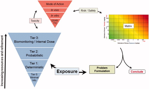
Table 1. Description of exposure tiers and examples of corresponding tools/models/data.

Tier	Description	Examples of exposure tools/models/databases^a	Websites (where applicable)
Tier 0	Limited information and/or limited use knowledge. Exposure estimates based primarily on physicochemical properties and route of exposure. May include estimates for:  • Humans indirectly exposed via the environment   ^ food, water, and/or air intake estimates   ^ water solubility and saturation vapor pressure data   ^ humans indirectly exposed via the environment banding look-up tables  • Consumer uses   ^ product use estimates   ^ consumer banding look-up tables  • Industrial uses   ^ manufacturing use estimates   ^ worker exposure banding look-up tables	physicochemical properties	http://java.epa.gov/chemview; http://webbook.nist.gov/chemistry/
		EPI Suite	http://www.epa.gov/opptintr/exposure/pubs/episuite.htm
		ChemIDPlus	http://chem.sis.nlm.nih.gov/chemidplus/
		SPIN	http://195.215.202.233/DotNetNuke/default.aspx
		Exposure look-up tables	Developed in this publication
		Environmental monitoring databases	See Table 7
Tier 1	Limited use knowledge. Exposure estimates based on results from exposure models with inputs for population, exposure route, environmental fate, volume, release, and specific-use and/or geometric mean values from monitoring databases	ECETOC TRA	http://www.ecetoc.org/tra
		ESIG GES EGRET	http://www.esig.org/en/regulatory-information/reach/ges-library/consumer-gess
		USETox	http://www.usetox.org
		SCI-GROW	http://www.epa.gov/oppefed1/models/water/scigrow_description.htm
		ChemSTEER	http://www.epa.gov/opptintr/exposure/pubs/chemsteer.htm
		E-FAST	http://www.epa.gov/opptintr/exposure/pubs/efast.htm
		ConsExpo	http://www.rivm.nl/en/Topics/C/ConsExpo
		SHEDS-HT	https://www.epa.gov/chemical-research/stochastic-human-exposure-and-dose-simulation-sheds-estimate-human-exposure
		RAIDAR	http://www.arnotresearch.com/index_download1.html#!/page_Downloads
		EUSES	https://ec.europa.eu/jrc/en/scientific-tool/european-union-system-evaluation-substances
Tier 2	Detailed use knowledge. Exposure estimates based on specific contaminant monitoring and measurement data used with probabilistic modeling.	PRZM-EXAMS	http://www.epa.gov/oppefed1/models/water/models4.htm#przm
		ConsExpo	http://www.rivm.nl/en/Topics/C/ConsExpo
		SHEDS	https://www.epa.gov/chemical-research/stochastic-human-exposure-and-dose-simulation-sheds-estimate-human-exposure
		ART	https://www.advancedreachtool.com/
Tier 3	Extensive knowledge. Exposure estimates based on internal dose, biomonitoring information, specific contaminant monitoring and measurement data.	National Report on Human Exposure to Environmental Chemicals	http://www.cdc.gov/exposurereport/
		Canadian Health Measures Survey	http://www.statcan.gc.ca/imdb-bmdi/5071-eng.htm
		Demonstration of a Study to Coordinate and Perform Human Biomonitoring on a European Scale	http://ec.europa.eu/environment/life/project/Projects/index.cfm?fuseaction=search.dspPage&n_proj_id =3759

^a ART: advanced REACH tool; ChemSTEER: chemical screening tool for exposures and environmental releases; EPI: estimation program interface; ECETOC: European Centre for Ecotoxicology and Toxicology of Chemicals; EGRET: European solvents industry group (ESIG) generic exposure scenario (GES) risk and exposure tool; EUSES: European Union system for the evaluation of substances; EXAMS: exposure analysis modeling system; E-FAST: exposure and fate assessment screening tool; PRZM: pesticide root zone model; RAIDAR: risk assessment, identification and ranking model; SCI-GROW: screening concentration in ground water; SPIN: substances in preparations in the Nordic countries; SHEDS-HT: stochastic human exposure and dose simulation-high throughput; TRA: targeted risk assessment.

Once the hazard and exposure estimates are obtained at the entry level tier, the next step is to combine the values graphically to assess human risk on the Risk Assessment Matrix shown in Figure 2. If the risk result falls into the lower left portion of the matrix, the conclusion is that the risk is low (A). If the risk result falls in the upper right portion of the matrix (B1), then refinement may be warranted. A decision can be made at this step to refine only the toxicity estimate, to refine only the exposure estimate, to refine both to facilitate decision making, or to act upon the available information as presented in the initial estimation.

Figure 2. Risk assessment matrix. Coloring indicates gradations of risk potential, from exposure being much lower than the hazard benchmark level (dark green, bottom left, including estimate (A) to exposure exceeding the hazard benchmark level (dark red, upper right, including estimate (B1). Estimate B2 illustrates a refinement of both exposure and toxicity that results in a range that is lower than the hazard benchmark.

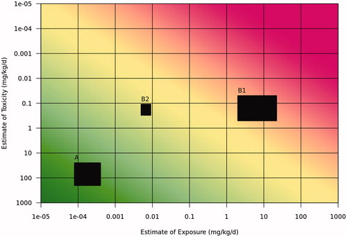
If a refinement is considered necessary, then additional information must be employed to better characterize exposure, toxicity, or both. Figure 2 illustrates the higher tier estimate (B2) resulting from refinement of both exposure and toxicity, which is plotted and compared with the acceptable risk range using the Risk Assessment Matrix. A risk decision is then made or further refinement is conducted, if deemed necessary and feasible.

2. Tier 0 exposure assessment using minimal information

Minimal exposure information, such as that described in Table 1 and elaborated in this section, can be used to make Tier 0 exposure estimates. Using physicochemical properties and basic exposure models, bands (groups) of screening type exposure estimates can be produced with limited information. This exposure banding methodology was conducted for worker, consumer, and indirect exposure to humans via the environment exposure scenarios and is described herein to provide Tier 0 exposure estimates.

2.1. Tier 0 using physicochemical properties for exposure estimates

The key characteristics that drive the environmental fate of a substance are state, structure and reactivity. Measures of hydrophobicity (Log K_ow value), kinetics and volatility (vapor pressure) can be used to estimate exposure. The physical state (liquid or solid) of a substance under specific conditions (e.g. environmental conditions or manufacturing process conditions) can be identified by using the melting/freezing point together with vapor pressure information. The melting point can give an indication about the relevant environmental compartment for the substance (air, water, soil) and boiling point information together with the vapor pressure data provide indications whether a substance may be available for inhalation as a vapor or may form flammable/explosive vapor-air mixtures.

There are several sources for physicochemical information. The NIST Chemistry WebBook (http://webbook.nist.gov/chemistry/) provides detailed information about chemical structure and chemical reactivity. ChemIDplus, http://chem.sis.nlm.nih.gov/chemidplus/chemidlite.jsp, is a free web search system that provides access to the structure and nomenclature authority files used for the identification of chemical substances cited in National Library of Medicine (NLM) databases with direct links to resources at NLM, federal agencies, U.S. states and scientific sites, including physicochemical properties. The EPI (Estimation Programs Interface) Suite™ is a Windows®-based suite of physical/chemical property and environmental fate estimation programs developed by the EPA’s Office of Pollution Prevention Toxics and Syracuse Research Corporation (SRC) as a screening tool (U.S. EPA 2011a). Likewise, the Exposure Toolbox in the Substances in Preparations In the Nordic countries (SPIN) database (http://eng.mst.dk/topics/chemicals/assessment-of-chemicals/spin-database/) contains information about chemical characteristics and properties along with other information that can be useful for developing a general indication of exposure to humans and the environment from different chemical uses.

Basic physical and chemical information incorporated into models can be used to prioritize chemicals, focus exposure assessments on specific environmental media, and, when used in conjunction with generic assumptions about exposure pathways, establish chemical-specific screening levels (U.S. EPA 1992). Likewise, the Organization for Economic Co-operation and Development (OECD) Environment Monograph no. 70 describes several approaches and models that can be used for screening purposes to estimate realistic levels of occupational or consumer exposure (Devine 1993; OECD 1993). Approaches on the use of physical chemical properties to consider or exclude certain exposure pathways are discussed in the Registration, Evaluation, Authorization and Restriction of Chemicals (REACH) guidelines (ECHA 2013) and in chemical safety information programs such as Chemview (http://www.epa.gov/oppt/existingchemicals/pubs/chemview.html). When utilizing physicochemical properties to screen for exposure potential, the media and use of the substance must be considered and aligned with the problem being assessed. For example, uses with elevated temperatures for substances with low vapor pressure can impact inhalation exposure potential. In some cases, upper bound exposures can be developed using equations that predict saturated vapor concentrations based upon vapor pressure, or water solubility as a maximum water concentration.

2.2. Tier 0 using look-up tables of exposure banding values

Exposure potential may be determined for workers, consumers, and to humans indirectly via the environment by utilizing the lowest tier exposure models such as those developed to comply with REACH legislation (ECHA 2012a, 2012b, 2012c). These models are useful for rapidly determining exposure because the output estimates are based on input parameters, such as physicochemical properties, that are categorized (banded). In this paper, this concept is referred to as “exposure banding.”

The European Centre for Ecotoxicology and Toxicology of Chemicals Targeted Risk Assessment (ECETOC TRA) tool, the European Solvent Industry Group’s Generic Exposure Scenario Risk and Exposure Tool (EGRET), and USEtox^® were used to generate very simple and logical charts for exposure banding (herein referred to as “look-up tables”). These look-up tables were developed assuming conservative exposure scenarios, require minimal data to use and provide exposure estimates in substantially reduced time as compared to if a source model was used outright.

2.2.1. Development of tier 0 occupational exposure bands

The ECETOC TRA v.3.1 worker module predicts short-term and long-term inhalation and dermal exposures for both solids and volatiles under industrial and professional exposure scenarios for all but a few of the process categories (PROCs) listed in the REACH guidance document (ECHA 2010). As described in REACH guidance, PROCs are used to categorize different technical processes applied during manufacturing and occupational use of substances and preparations. The PROCs may be applied in industrial settings, such as during manufacturing or formulation of the substance or preparation, or in professional settings, such as when craftsmen use the substance or preparation.

The exposure predictions are based on both the PROC and on the fugacity of the substance or preparation. Fugacity in this context is defined as “the inherent tendency of a substance to become airborne” (ECETOC 2004). In the ECETOC TRA v.3.1 worker module, fugacity is banded into four vapor pressure bands (negligible VP (< 0.01 Pa), low VP (≥ 0.01 < 500 Pa), medium VP (≥ 500 ≤ 10 000 Pa), high VP (> 10 000 Pa)) and three dustiness levels (low, medium, high). For inhalation exposures to volatiles, model output depends only upon vapor pressure; however, for inhalation exposure to solids, the exposure prediction is a function of the dustiness level.

In this study, a molecular weight of 100 g/mol was assumed to generate a standard look-up table and the worst-case ventilation level (indoor ventilation) was applied for all exposure scenarios for industrial workers (Table 2) and for professional workers (Table 3). For inhalation exposure, the long-term (LT) estimates are presented in ppm for volatiles and in mg/m³ for solids. The short-term (ST) estimates for both solids and volatiles are in mg/m³. For dermal exposure, Tables 2 and 3 include exposure estimates for long-term systemic (mg/kg/day) and long-term local endpoints (μg/cm²) for each PROC.

Table 2. Industrial worker exposure look-up table from ECETOC TRA v.3.1 Model.

Table 2. Continued.

Table 3. Professional worker exposure look-up table from ECETOC TRA v.3.1 model.

Table 3. Continued.

In an inhalation exposure assessment, the look-up table values for solids can be directly used as they are independent of the substance molecular weight (MW). However, the volatiles look-up values must be adjusted before comparing the predictions with the occupational exposure limits (OELs). These adjustments are as follow:

ST exposure adjustment for MW (1)

LT exposure adjustment for units (when conversion from ppm to mg/m³ is necessary) (2)

It should be noted that the dermal estimates are the same for any substance regardless of physicochemical properties; therefore, the dermal look-up estimates can be used directly without making a MW adjustment.

These look-up tables were further modified to develop a step-wise procedure for conducting an exposure assessment. Two different example approaches (A and B) were designed and employed for industrial workers to test the utility of the look-up tables. The steps for these approaches are described in Box 1. To meet user-specific circumstances, procedures other than the ones illustrated below may be developed to conduct the occupational exposure assessment.

Box 1. Tier 0 exposure assessment – worker look-up table example procedures.

After each step in Approach A Example or Approach B Example, if the exposure estimate is < the Occupational Exposure Limit (OEL), no additional action is taken; if the exposure estimate is > the OEL, then proceed to the next step.
Approach A Example
STEP 1: Determine from the look-up table the exposure estimates for the sentinel (worst-case) PROCs. ASSUME the highest fugacity (vapor pressure for volatiles or dustiness for solids) for the substance unless already KNOWN (Tables 2 and 3 list all of the PROCs with the sentinel PROCs highlighted).
STEP 2: Where required, complete the MW and unit adjustments for the look-up estimates. (Equations (1)(1) and (2)(2) )
STEP 3: Compare the Step 2 estimates with the Occupational Exposure Level (OEL).
If , then the substance warrants additional analysis.
STEP 4: Identify relevant PROCs from site personnel. If data are available consider KNOWN fugacity levels. Perform Steps 2 and 3 again for relevant PROCs.
STEP 5: From site personnel identify the ventilation level associated with each relevant PROC. Determine exposure estimate(s) by manually applying the reduction factor associated with each relevant PROC at that ventilation level as defined by ECETOC 2012. Perform Steps 2 and 3 again. (Limitation of exposure duration, use of personal protection equipment, and accounting for the concentration of the substance are additional controls or measures that may be used in combination or individually to reduce the exposure estimates in Step 5. The use of the ventilation level in this example test case was for illustrative purposes only.)
Approach B Example
STEP 1: Use fugacity for the substance and apply the adjustments (MW and unit) to determine from the look-up table all PROC(s) with exposure estimate(s) < OEL. Mark them GREEN.
STEP 2: Assign a Prioritization Rank as follows dependent on which PROCs are labeled GREEN in Step 1. (The assignment of ranks 0 through 3 to particular PROCs in this example test case was for illustrative purposes only. The assignment of a PROC to a particular rank may be modified to meet the user’s specific circumstances. In addition more or less ranking categories than illustrated here may be created by the user.)
3 = No PROCs or only PROC 1< OEL = HIGH priority for higher tier risk assessment
2 = PROCs 8b or 9 not < OEL = MEDIUM priority for higher tier risk assessment
1 = Not already assigned a Risk Rank of 3, 2, or 0= LOW priority for higher tier risk assessment
0 = All PROCs < OEL = Consider eliminating from higher tier risk assessment

Approach A was applied to eight different substances for which some exposure information was available, but at varying levels (see Supplemental Tables A1–A3). Substance molecular weights and OELs were also known when testing Approach A. Had OELs not been available, some hazard level, such as Threshold of Toxicological Concern (TTC) (Munro et al. 1996; Barlow 2005) would have been used for comparison to the exposure estimates. For the eight substances tested using Approach A, the physical state and fugacity assumptions were conservative. Based on this minimal information, initial exposure estimates were obtained using only the sentinel PROCs (PROC 7 for inhalation and PROC 19 for dermal) from the look-up table. For this initial estimate, only one of eight substances was found to present significantly lower exposure estimates than the corresponding OEL (Step 3, output). Since more information regarding the applicable PROCs and the actual fugacity levels for these substances was available, refined estimates were made and an additional substance was eliminated from the list after Step 4. Information on relevant ventilation levels were gathered to further refine the estimates for each identified PROC; this exercise however, did not remove any additional substances. The results of Approach A are included in the Supplemental information as Tables A1 through A3.

Approach B was used on a much larger group of substances (∼130) for which essentially no exposure information was known. Only substance molecular weight, fugacity level and OELs were known. With implementation of Approach B, approximately 14% of the substances analyzed suggested that elimination from higher tier risk assessment was appropriate. Likewise, it was relatively easy to rank the remaining 110 substances into three distinct groups; an additional 13% were categorized with a LOW priority definition, 16% fell under a MEDIUM priority definition, and the remaining 57% of the substances were categorized as HIGH priority after completing Approach B. The results of Approach B are included in the Supplemental information as Tables A4 through A7.

2.2.2. Development of tier 0 consumer exposure bands

Similar to the work described under occupational exposure bands, a parallel analysis was done to investigate the possibility of developing consumer exposure look-up tables based upon use and physicochemical properties. The two tools selected for this analysis were ECETOC TRA v.3 consumer module and EGRET. Similar to the TRA-worker module approach, four vapor pressure bands were defined in both TRA-consumer and EGRET models: low VP (<0.1 Pa), medium low VP (≥0.1 < 1 Pa), medium VP (≥1 < 10 Pa), and high VP (≥10 Pa). The inhalation exposure predictions for nonspray application were driven by the vapor pressure band; dermal and oral ingestion estimates, however, are independent of physical chemical properties. The exposure routes in both tools have been pre-determined based on whether they are relevant to the scenario.

To generate look-up tables, both TRA and EGRET were run with no modification to defaults. The ECETOC TRA-consumer module was run in a straight forward manner by selecting all the product categories (PC) and article categories (AC) at four different vapor pressure values, one from each vapor pressure band. These PCs and ACs describe the chemical product type and the type of article that will finally contain the substance when supplied to the end uses (ECHA 2012b). The molecular weight was left blank so that saturated vapor pressure concentration was not invoked as an upper bound for inhalation exposure. For EGRET, the initial molecular weight and vapor pressure values were set so that the saturated vapor concentration exceeded exposure predictions based upon the model defaults. Thus, predictions were not bounded by substance-specific physical chemical factors that determined saturated vapor concentration.

The exposure estimates obtained by these models were in mg/m³ and mg/kg/day for inhalation exposures, and in mg/kg/day for oral and dermal exposures. For the development of look-up tables, only mg/kg/day estimates were utilized so that total exposures could be added across routes. ECETOC TRA v.3 exposure estimates are provided for day of use; EGRET offers multiple options for reporting exposure concentrations depending upon averaging time: per event, per day of use, or on a chronic basis. Look-up tables were developed for day of use as this averaging time was available for both models (Table 4 from TRA, Table 5 from EGRET). In a similar fashion, look-up tables could be developed for other time periods or by exposure routes (Supplemental Tables B1–B4). The look-up tables assisted in focusing exposure activities, for example, by identifying both sentinel products (those with greatest exposure potential within a product category, e.g. “glue from spray” subcategory with the highest total exposure is a sentinel product for PC1 in Figure 3) or by focusing further refinement on exposure routes that contribute the most to total exposure (e.g. inhalation is a dominant exposure route for PC1 “glue from spray” scenario in Figure 3). Preliminary comparison of a limited number of ECETOC TRA v.3 and EGRET predictions with higher tier predictions (ConsExpo) or measured values was also performed (Zaleski et al. 2014) and found that these models are conservative and generally have similar trends in relative exposure values across scenarios. As the EGRET tool represents the TRA with additional refinements, the exposure values obtained may be less conservative yet sufficient for decision making,

Figure 3. Consumer exposure estimation for products at low vapor pressure derived from EGRET tool.

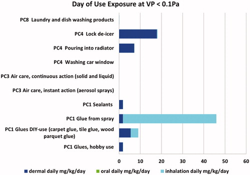
Table 4. Tier 0 consumer exposure (ECETOC TRA v.3), acute (day of use) exposure estimates by vapor pressure.

		Total predicted exposure (mg/kg/d) - day of use
Descriptor	Product subcategory	<0.1 Pa	0.1 – <1 Pa	1 – < 10 Pa	≥10 Pa
PC1: Adhesives, sealants	Glues, hobby use	1.8	1.8	2.2	5.4
	Glues DIY-use (carpet glue, tile glue, wood parquet glue)	28.1	88.5	692.4	6731.4
	Glue from spray	104.8	104.8	104.8	104.8
	Sealants	1.9	3.4	17.5	158.8
PC3: Air care products	Aircare, instant action (aerosol sprays)	5.0	5.0	5.0	5.0
	Aircare, continuous action (solid & liquid)	0.1	0.1	0.8	7.9
PC9a: Coatings, paints, thinners, removers	Waterborne latex wall paint	37.7	56.0	238.7	2065.7
	Solvent rich, high solid, water borne paint	36.4	42.7	106.1	739.7
	Aerosol spray can	47.2	47.2	47.2	47.2
	Removers (paint-, glue-, wall paper-, sealant-remover)	131.4	153.2	371.0	2549.0
PC9b: Fillers, putties, plasters, modelling clay	Fillers and putty	7.3	19.4	140.0	1346.0
	Plasters and floor equalizers	169.0	403.0	2743.0	26143.0
	Modelling clay	35.4	35.4	35.4	35.4
PC9c: Finger paints	Finger paints	194.5	194.5	194.5	194.5
PC12: Fertilizers	Lawn and garden preparations	86.5	86.5	86.5	86.5
PC13: Fuels	Liquids	74.9	105.1	407.5	3431.5
PC24: Lubricants, greases, and release products	Liquids	74.9	105.1	407.5	3431.5
	Pastes	28.6	28.6	28.6	28.6
	Sprays	237.7	237.7	237.7	237.7
PC31: Polishes and wax blends	Polishes, wax/cream (floor, furniture, shoes)	71.9	75.2	108.5	441.5
	Polishes, spray (furniture, shoes)	162.2	162.2	162.2	162.2
PC35: Washing and cleaning products (including solvent based products)	Laundry and dish washing products	85.8	86.0	87.9	107.2
	Cleaners, liquids (all purpose cleaners, sanitary products, floor cleaners, glass cleaners, carpet cleaners, metal cleaners)	71.5	71.9	75.4	110.8
	Cleaners, trigger sprays (all purpose cleaners, sanitary products, glass cleaners)	38.0	38.0	38.0	38.0
AC5: Fabrics, textiles and apparel	Clothing (all kind of materials), towel	1034.6	1037.7	1068.2	1373.3
	Bedding, mattress	27.9	63.4	418.0	3964.0
	Toys (cuddly toy)	56.7	56.7	56.7	56.7
	Car seat, chair, flooring	148.5	171.2	398.0	2666.0
AC6: Leather articles	Purse, wallet, covering steering wheel (car)	0.7	1.0	3.4	27.6
	Footwear (shoes, boots)	3.6	4.7	16.1	129.5
	Furniture (sofa)	15.9	28.0	148.6	1354.6
AC8: Paper articles	Diapers	55.7	55.7	55.7	55.7
	Sanitary towels	7.2	7.2	7.2	7.2
	Tissues, paper towels, wet tissues, toilet paper	28.6	28.6	28.7	29.4
	Printed paper (papers, magazines, books)	4.2	8.4	51.0	476.7
AC10: Rubber articles	Rubber handles, tyres	6.1	54.5	538.7	5380.7
	Flooring	6.0	28.7	255.5	2523.5
	Footwear (shoes, boots)	3.6	4.7	16.1	129.5
	Rubber toys	2.3	2.3	2.3	2.3
AC11: Wood articles	Furniture (chair)	14.8	16.4	32.1	189.6
	Walls and flooring (also applicable to non-wood materials)	5.9	27.2	239.6	2363.6
	Small toys (car, train)	2.3	2.3	2.3	2.3
	Toys, outdoor equipment	6.6	6.6	6.6	6.6
AC13: Plastic articles	Plastic, larger articles (plastic chair, PVC-flooring, lawn mower, PC)	68.1	116.9	604.7	5482.7
	Toys (doll, car, animals, teething rings)	24.3	24.3	24.3	24.3
	Plastic, small articles (ball pen, mobile phone)	1.0	1.5	6.1	51.8

Table 5. Tier 0 consumer exposure (EGRET) predictions, acute (day of use) exposure estimates from EGRET by vapor pressure.

		Total predicted exposure (mg/kg/d) – day of use
Product category	Product subcategory sentinels	< 0.1 Pa	0.1 – <1 Pa	1 – < 10 Pa	≥ 10 Pa
PC1: Adhesives, sealants	Glues, hobby use	1.79	1.83	2.25	6.46
PC1: Adhesives, sealants	Glues DIY-use (carpet glue, tile glue, wood parquet glue)	9.05	40.98	360.3	3553.46
PC1: Adhesives, sealants	Glue from spray	45.93	45.93	45.93	45.93
PC1: Adhesives, sealants	Sealants	1.81	1.98	3.72	21.10
PC3: Air care products	Air care, instant action (aerosol sprays)	0.05	0.05	0.05	0.05
PC3: Air care products	Air care, continuous action (solid and liquid)	0.06	0.06	0.07	0.15
PC4_n: Anti-freeze and de-icing products	Washing car window	5.64E-08	5.64E-07	5.64E-06	5.64E-05
PC4_n: Anti-freeze and de-icing products	Pouring into radiator	7.13	7.14	7.23	8.14
PC4_n: Anti-freeze and de-icing products	Lock de-icer	18.15	18.15	18.15	18.15
PC8_n: Biocidal products (excipient use only for solvent products)	Laundry and dish washing products	0.07	0.08	0.11	0.44
PC8_n: Biocidal products (excipient use only for solvent products)	Cleaners, liquids (all purpose cleaners, sanitary products, floor cleaners, glass cleaners, carpet cleaners, metal cleaners)	7.15	7.15	7.19	7.61
PC8_n: Biocidal products (excipient use only for solvent products)	Cleaners, trigger sprays (all purpose cleaners, sanitary products, glass cleaners)	11.67	11.67	11.67	11.67
PC9a: Coatings, paints, thinners, paint removers	Waterborne latex wall paint	1.13	1.65	6.85	58.80
PC9a: Coatings, paints, thinners, paint removers	Solvent rich, high solid, water borne paint	19.94	22.5	48.18	304.96
PC9a: Coatings, paints, thinners, paint removers	Aerosol spray can	18.79	18.79	18.79	18.79
PC9a: Coatings, paints, thinners, paint removers	Removers (paint-, glue-, wall paper-, sealant-remover)	71.78	74.72	104.1	397.89
PC9b: Fillers, putties, plasters, modeling clay	Fillers and putty	0.12	0.15	0.41	3.06
PC9b: Fillers, putties, plasters, modeling clay	Plasters and floor equalizers	3.23	6.53	39.56	369.85
PC9b: Fillers, putties, plasters, modeling clay	Modelling clay	3.54	3.54	3.54	3.54
PC9c: Finger paints	Finger paints	194.7	194.7	194.7	194.70
PC12: Fertilizers	Lawn and garden preparations	86.46	86.46	86.46	86.46
PC13: Fuels	Liquid - subcategories added: Automotive Refueling	35	35.01	35.08	35.84
PC13: Fuels	Liquid - subcategories added: Scooter Refueling	35	35.01	35.06	35.56
PC13: Fuels	Liquid - subcategories added: Garden Equipment - Use	0.004	0.04	0.4	3.99
PC13: Fuels	Liquid (subcategories added): Garden Equipment - Refueling	70	70	70.04	70.44
PC13: Fuels	Liquid (subcategories added): Home space heater fuel	35	35	35.01	35.13
PC13: Fuels	Liquid - subcategories added: Lamp oil	35	35	35.01	35.07
PC15_n: Non-metal surface treatment products	Waterborne latex wall paint	1.13	1.65	6.85	58.80
PC15_n: Non-metal surface treatment products	Solvent rich, high solid, water borne paint	19.94	22.5	48.18	304.96
PC15_n: Non-metal surface treatment products	Aerosol spray can	18.79	18.79	18.79	18.79
PC15_n: Non-metal surface treatment products	Removers (paint-, glue-, wall paper-, sealant-remover)	71.78	74.72	104.1	397.89
PC16_n: Heat transfer fluids	Liquids	78	78.02	78.22	80.22
PC17_n: Hydraulic fluids	Liquids	78	78.02	78.22	80.22
PC18_n: Ink and toners	Inks and toners	1.2	1.25	1.75	6.77
PC23_n: Leather tanning, dye, finishing, impregnation and care products	Polishes, wax/cream (floor, furniture, shoes)	35.86	36.11	38.61	63.64
PC23_n: Leather tanning, dye, finishing, impregnation and care products	Polishes, spray (furniture, shoes)	45.4	45.4	45.4	45.40
PC24: Lubricants, greases, and release products	Liquids	78	78.02	78.22	80.22
PC24: Lubricants, greases, and release products	Pastes	15.6	15.6	15.6	15.60
PC24: Lubricants, greases, and release products	Sprays	42.46	42.46	42.46	42.46
PC27_n: Plant protection products		86.46	86.46	86.46	86.46
PC31: Polishes and wax blends	Polishes, wax/cream (floor, furniture, shoes)	35.9	36.54	42.88	106.34
PC31: Polishes and wax blends	Polishes, spray (furniture, shoes)	41.81	41.81	41.81	41.81
PC34_n: Textile dyes, finishing and impregnating products		0.15	0.24	1.13	10.02
PC35: Washing and cleaning products (including solvent based products)	Laundry and dish washing products	0.07	0.08	0.11	0.44
PC35: Washing and cleaning products (including solvent based products)	Cleaners, liquids (all purpose cleaners, sanitary products, floor cleaners, glass cleaners, carpet cleaners, metal cleaners)	7.15	7.15	7.19	7.61
PC35: Washing and cleaning products (including solvent based products)	Cleaners, trigger sprays (all purpose cleaners, sanitary products, glass cleaners)	11.67	11.67	11.67	11.67
PC36_n: Water softners		0.002	0.002	0.002	0.002
PC37_n: Water treatment chemicals		0.02	0.02	0.02	0.02
PC38_n: Welding and soldering products, flux products		0.002	0.02	0.21	2.06

The authors envision that a Tier 0 consumer risk screening approach utilizing these types of look-up tables would have the steps discussed in Box 2. In all cases, default exposure assumptions should be evaluated to determine if they are appropriate for the use being assessed. As the consumer tool algorithms result in exposure predictions that are directly linearly proportional to weight fraction, the table’s utility could be expanded by providing more realistic upper bound concentrations related to functional category – for example, fragrance, colorant, or surfactant functional ingredients may have upper band weight fractions that differ from the TRA and EGRET defaults.

Box 2. Tier 0 exposure assessment – consumer look-up table procedures.

STEP 1: Choose representative category and subcategories.

STEP 2: Evaluate scenario assumptions to see if they apply to the problem being studied. If relevant, proceed to step 3; if not relevant, go to a higher tier approach.

STEP 3: If scenario is appropriate for purpose, use look-up table as upper bound exposure. This exposure value can be compared to a hazard benchmark to determine if additional evaluation is needed.

The following activities could help expand its scope to cover additional product types and exposure scenarios: Default values for existing scenarios can be refined and this can be focused by using the information provided in Tables 4 and 5 to identify sentinel products (ones with greatest exposure potential) and exposure routes driving predictions for a given scenario. Scenarios can be added. Weight fractions (product ingredient) could be adjusted by functional purpose (for example, a surfactant may have a maximum weigh fraction of x, whereas a solvent maximum weight fraction may be y, and a colorant may be z). Additional physical chemical properties could be considered as appropriate.

2.2.3. Development of tier 0 exposure bands for humans indirectly exposed via the environment

2.2.3.1. Previous banding approach and need for a banding approach for human exposure.

Verdonck et al. (2005) developed look-up tables to identify potential environmental risk based on ecotoxicity. They used the European Union System for the Evaluation of Substances (EUSES) model to identify the key input parameters and produced a simple look-up table that provides banded risk characterization ratios (RCRs, or the ratio of the predicted environmental concentration to the predicted no effect concentration) based on dichotomous classes of release scenario (production or private use), biodegradability (readily or nonbiodegradable), log vapor pressure (−2 to 0, or 0 to 6), and log Kow (0 to 5, or 5 to 7). The predicted exposures were determined assuming a default emission of 1 tonne/year and an ecotoxicity threshold of 1 μg/l, but the values scale linearly with emission tonnage and the hazard benchmark value. Building upon the idea of exposure banding, there is a need to develop an approach for human indirect exposure banding that encompasses the multiple human exposure pathways based on a systematic analysis of exposure model results for a wide range of chemicals. The following section develops such a banding approach for human exposure based on an analysis of multipathways intake fractions.

2.2.3.2. Banded table based on human intake fraction for tier 0 estimates.

A number of fugacity-based mass balance models are available to quantify the fate, transport, and transformation of organic chemicals in the environment (Arnot et al. 2006; Rosenbaum et al. 2008), and eventually, the intake fraction (iF) that characterizes human intake through direct (e.g. inhalation, drinking water ingestion) and indirect (e.g. food bioaccumulation) pathways. The intake fraction represents the fraction of the chemical emitted that is eventually taken in by the human population and depends upon emission route, physical–chemical properties, environmental characteristics and human population density (Bennett et al. 2002). These models recently have been applied to several thousand compounds (20 000 in one case) by various groups (Rosenbaum et al. 2008; Arnot et al. 2012; Wambaugh et al. 2013), to determine intake fractions for screening purposes. Among these models, USEtox, the UNEP-SETAC toxicity consensus model, has been developed as a parsimonious consensus model whose outputs falls within the output range of other existing characterization models (Hauschild et al. 2008). Work has also been completed to identify the key parameters influencing USEtox intake fractions (Henderson et al. 2011), but so far USEtox or other multimedia models have not been applied to band intake fractions.

To address human risk based on indirect exposure through the environment, a table of banded intake fractions was developed using the USEtox model (Rosenbaum et al. 2008) accounting for human inhalation and ingestion exposures as additional chemical removal pathways.

USEtox intake fractions were estimated for emissions into urban air, continental rural air and continental freshwater, for three exposure pathways: inhalation (iF_inh), fish consumption (iF_fish), and non-fish dietary ingestion (iF_{nf - ing}) including drinking water, above and below ground crops, meat and dairy consumption. The iF estimates were obtained from the USEtox mass balance multi-media model by Rosenbaum et al. (2008), and physicochemical properties from EPI Suite 4.10 for 3,073 substances (U.S. EPA 2011a). To calculate maximum intake fractions, emissions were assumed to be dispersed into air (urban or continental rural) for inhalation and the rest of ingestion, but for fish consumption, emissions were assumed to be dispersed into continental freshwater. Key chemical properties that mostly affect intake fractions were identified to categorize these intake fractions and provide upper bounds for iFs and consequently for indirect human exposure estimates.

Figure 4 illustrates the results of this banding for inhalation, fish consumption, and ingestion exposure pathways. Banded intake fractions are summarized in Table 6 as a function of four physicochemical properties: the half-life in air (t_½,air, d), the octanol-to-water partition coefficient (K_ow), the octanol-to-air partition coefficient (K_oa), and the fish bioaccumulation factor (BAF_fish) as derived by EPI Suite, incorporating prediction of apparent metabolism half-life in fish, and estimating BAF for three trophic levels. As the potential amount of an environmental release that is taken up by the human population depends upon the population density, iF were developed for both rural and urban releases (with urban density of two million people over 240 km², rural density of six billion people over 9 000 000 km², respectively).

Figure 4. Intake fractions and upper limits of iFs as a function of key chemical properties: (a) Upper limits for the inhalation iF for emissions into urban and continental rural air as a function of half-life in air, (b) Upper limits for the fish consumption iF for emissions into continental freshwater as a function of the bioaccumulation factor in fish and (c) Upper limits for the non-fish ingestion iF for emissions into rural air as a function of the octanol-air partition coefficient, for different values of the octanol-water partition coefficient.

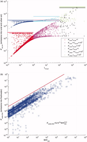
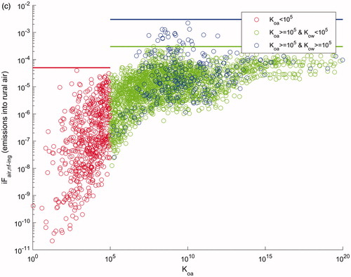
Table 6. (a) Upper limits for intake fraction and (b) high-end exposure and variability factors, per environmental exposure pathway.

(a) Intake fractions upper limits for dichotomous classes of half lives in air (t1/2 air), bioaccumulation factors (BAFfish), octanol-air and octanol water partition coefficients.
Inhalation			Fish consumption	Nonfish dietary ingestion
	Upper iFinh limit
Condition	Rural	Urban	Upper iFfish limit	Condition	Upper iFnf-ing limit
t1/2 air≤1 d	3 × 10^- 6	3 × 10^- 5	iF =5 × 10^−6 × BAFfish^0.91	Koa<10^5	5 × 10^- 5
1<t1/2 air≤100 d	3 × 10^- 5	6 × 10^- 5		Koa≥10^5 and Kow<10^5	3 × 10^- 4
t1/2 air>100 d	3 × 10^4	3.5 × 10^- 4		Koa≥10^5 and Kow ≥10^5	3 × 10^- 3
(b) high-end exposure and spatial variability factors.
Exposure pathway	Inhalation		Fish consumption	Nonfish dietary ingestion
	Inh		fish	nf-ing
High-end exposure factor HC	1.5*		2.2†	2*
Spatial variability factor SV	6‡		20¶	10¶

* Ratio of the 95th to average intakes taken from the Exposure Factors Handbook (EPA 2011).

† Ratio of the 95th from the Exposure Factors Handbook to average USEtox fish consumption.

‡ Based on urban spatial variability of ground level PM_2.5 intake fractions, calculated as the ratio of the highest urban iF in the world (2.6 × 10^{- 4}) according to Apte et al. (2012), compared to the typical city selected in USEtox (4.4 × 10^{- 5}).

¶ Based on Pennington et al. (2005, Figures 4 and 5), for distributed emissions of persistent substances with high intake fraction, that best correspond to this banding exercise.

Figure 4(a) illustrates how the inhalation iF to urban air (.) and continental rural air (+) is capped as a function of the half-life in air (t_½,air). Substances were divided into three bins depending on the atmospheric persistency of the substance: half-life in air less than a day, a day to 100 days, and more than 100 days. For urban air emissions, the inhalation iF upper limits were calculated to be 3 × 10⁻⁶, 3 × 10⁻⁵, and 3 × 10⁻⁴ kg_in/kg_emitted, while for continental, rural air emissions were 3 × 10⁻⁵, 6 × 10⁻⁵, and 3.5 × 10⁻⁴ kg_in/kg_emitted, respectively.

Figure 4(b) shows that the fish consumption iF for continental freshwater emissions is capped as a function of the fish bioaccumulation factor. Data are capped by the straight line on the log-log scale given by iF_fish = 5 × 10⁻⁶×BAF_fish^0.91. The BAF values reported in EPI Suite led to relatively high iFs for bio magnificating compounds, up to 10⁻¹.

Figure 4(c) illustrates how the nonfish dietary iF varied as a function of the octanol-air partition coefficient (K_oa). For banding, the octanol-water partition coefficient (K_ow) was used to identify the high bioconcentrating substances in above-ground produce. For both chemical properties, 10⁵ was used as a cutoff point creating three categories for the substances tested, with an upper limit iF of 5 × 10⁻⁵ kg_in/kg_emitted for K_oa<10⁵, an upper iF of 3 × 10⁻⁴ for K_oa≥10⁵ and K_ow <10⁵, and an upper iF of 3 × 10 ⁻³_, for K_oa≥10⁵ and K_ow ≥10⁵.

2.2.3.3. Application of banded iF for estimating tier 0 environmentally mediated human exposures.

Application of this model requires knowledge of the environmental release mass and population size to develop an estimate of the amount taken up by an individual from an iF value. From the upper intake fractions in Table 6(a), an upper human dose from environmental exposures was calculated (Dose_{Tier 0}, mg/kg/day) for a given substance by the following equation: (3) where S_{tier 0} in mg/kg/day is the substance daily emitted mass normalized per kg body weight, iF_i in kg_in/kg_emitted is the population intake fraction for each exposure pathway i (i = inh, fish, nf-ing) from Table 6, HC (dimensionless) is a pathway specific factor to account for high-end exposures (USEtox is based on average inhalation and ingestion rates) and SV (dimensionless) is a pathway specific factor accounting for the spatial variability of intake fraction, with values used for development of look up tables, selected to provide an additional degree of conservatism for the purposes of this exercise, given for HC and SV in Table 6(b). As a range, the results were considered with and without the high end exposure and spatial variation factors, since for chronic effects, average annual values may be more representatives.

When emissions are unknown, a proxy of the substance daily emitted mass normalized per kg body weight can be calculated from the annual substance production volume (PV, in kg/year, from, e.g. the 2006 U.S. EPA Inventory Update Reporting and Chemical Data Reporting http://www.epa.gov/oppt/cdr/index.html), as applied by Wambaugh et al. (2013) and Shin et al. (2015). It is normalized by the considered population and body weight as follows: (4)

This is a first attempt to apply the banding approach on iF for assessing indirect human exposure due to environmental releases. The results should be interpreted with caution since it is does not necessarily represent exposures at sites in close proximity to point sources. As discussed by Shin et al. (2015), production volume does not accurately represent environmental release amounts but is only a rough approximation, especially for chemicals used as intermediary reactants in manufacturing.

Since chemical properties can be estimated by chemical structure alone using QSARs available with computer packages such as EPA’s Estimation Program Interface (EPI) Suite v4.10 (http://www.epa.gov/oppt/exposure/pubs/episuite.htm) (U.S. EPA 2011a), three approaches are possible to derive exposure estimates in decreasing degree of conservatism: (a) estimates of intakes directly based on physicochemical data such as water solubility or air vapor pressure at Tier 0, (b) application of the above developed banded iF as a more refined Tier 0 approach or (c) use of the results obtained by USEtox for the specific chemical can be used at the Tier 1 level. These three approaches are demonstrated in the case study discussed in Section 3.

2.3. Tier 0 using monitoring databases to inform on exposure

In addition to look-up tables, users can also utilize environmental monitoring databases to obtain the background concentrations of a substance in different exposure media (air, water, and/or food). For example, if humans may be exposed to the substance in question by ingestion (food and water) and inhalation (air), then existing monitoring data for food and air contamination can be considered to estimate possible concentrations in Tier 0 estimates. There are many databases that contain information concerning levels of substances in food, drinking water, and air such as the USDA Pesticide Data Program (http://www.ams.usda.gov/datasets/pdp) and the US EPA SDWIS (http://www3.epa.gov/enviro/facts/sdwis/search.html) database. The scope and the background of a few of the potential data sources by route, that is, food, drinking water, and air are summarized in Table 7. It is important to note that the use of monitoring database information is complex and requires proper understanding of the principal criteria used to establish the database. Existence of a unique source or particular physicochemical characteristic not consistent with the exposure scenario at hand would preclude the use of that database value. It is recommended that users consider the following suggestions if using data from a monitoring database for an exposure assessment:

Table 7. Summary of monitoring databases.

		Highest observed value
Exposure media	US database	Value (chemical)	Unit	# Chemicals analyzed	# Analyses per chemical	Time period	Sample source	Website link
Food	USDA PDP	33	mg/L	>100 commodities >500 pesticides	Varies per type of commodity, range is 3000–15 000	1991–present	Food, beverages and other commodities	http://www.ams.usda.gov/AMSv1.0/pdpdata
Drinking Water	USDA PDP	0.034 (pesticide)	mg/L	490 pesticides 23 environmental contaminants 30 pharmaceuticals	2000–4000	1991–present	Drinking water (from ground or surface)	http://www.ams.usda.gov/AMSv1.0/pdpdata
	USGS NAWQA	20 (MTBE)	mg/L	31 Metals, 55 VOCs, 83 pesticides	2000–4000	1996–present	Ground and surface water	http://water.usgs.gov/nawqa/
	US EPA SDWIS Controlled Contaminant (review 1)	43 (Benzene)	mg/L	62 regulated substances	10 000–50 000	1990–1997	Drinking water (from ground or surface)	http://water.epa.gov/lawsregs/rulesregs/regulatingcontaminants/sixyearreview/sixyearoccurencedata/index.cfm
	US EPA SDWIS Controlled Contaminant (review 2)	5 (Toluene)	mg/L	62 regulated substances	10 000–50 000	1998–2005	Drinking water (from ground or surface)	http://water.epa.gov/lawsregs/rulesregs/regulatingcontaminants/sixyearreview/sixyearoccurencedata/index.cfm
	US EPA SDWIS Uncontrolled Contaminant	0.4 (Perchlorate)	mg/L	24 mostly pesticides	2000–4000	2001–2005	Drinking water (from ground or surface)	http://water.epa.gov/lawsregs/rulesregs/sdwa/ucmr/index.cfm
Air	WHO Database	279 (PM10)	μm/m3	PM2.5 - 10	Monitoring stations measuring frequently but only annual mean reported	2003–2010	Urban outdoor air	http://www.who.int/phe/health_topics/outdoorair/databases/en/
	AIRMEX Database	Indoor: 88 (limonene) Outdoor: 33(toluene)	μg/m3 μg/m3	14 VOCs	1000 samples collected	2004–2008	Indoor and outdoor air in Europe	http://ihcp.jrc.ec.europa.eu/our_databases/airmex
	EPA Air Quality Database			16 air quality parameters (e.g. CO, Pb, NOX, SOX, VOC, PM)	Very large, data from monitoring stations all over USA	1980–present	Outdoor air	http://www.epa.gov/ttn/airs/airsaqs/detaildata/downloadaqsdata.htm
	California Air Toxics Board Database			10 air quality parameters (e.g. CO, NO2, O3, SO2, H2S, Methanol, VOC)	Very large, data from monitoring stations all over CA	1980–present	Outdoor air	http://www.arb.ca.gov/aqd/aqdcd/aqdcddld.htm

• The user must understand the intended purpose of the database, the type of samples that were tested, and if the samples represent the use scenario.

• When selecting a worst case value from the database, consideration of the meaningfulness of the value is necessary, using physicochemical properties, distance to source, and mass of emission.

• Attention also needs to be paid to temporal aspects of the reported exposure value (i.e. is it an annual average, task value, etc.) and that they are matched to the temporal aspects developed in the initial problem formulation step.

• The intent of most water monitoring databases is to assess the quality of water in regards to specific regulations. In some cases it is the average that is typically used, and outliers typically have little effect. However, selecting a maximum value for exposure from these databases might end up being based on a value that was not validated.

• The evaluation of air monitoring databases may be more complex than food and water databases. It should be noted that measured concentrations in air can be specific to outdoor and/or indoor air environments and exposure sources as well as specific geographic locations and meteorological conditions. Thus in order to select one database to represent general environmental background, it is recommended to collect more information concerning the emission sources of the substance in question and the location and definition of the population of concern.

3. Case study

To demonstrate application of the banding-based tiered exposure assessment approach, an example follows below. Additionally, this case study illustrates the application of the RISK21 framework, starting with problem formulation, and the comparison of exposure and toxicity on the risk matrix for Tier 0, followed by Tier 1 exposure refinement.

This case study is linked to a related RISK21 case study (Doe et al. 2016). The Doe et al. case study focused on a new pyrethroid to be used for mosquito netting to protect against malaria and applied the RISK21 approach to minimize animal use and take advantage of existing toxicity and exposure information. In order to have toxicity information available to evaluate the banding-based tiered exposure assessment described herein, the case study described below utilizes deltamethrin, rather than a new pyrethroid, and a modified scenario.

3.1. Problem formulation

In this hypothetical scenario, an outdoor sports company has been requested by several highly attended children summer camps in Texas to provide mosquito netting to prevent the transmission of West Nile virus from mosquitoes while children (6–12 years old) sleep in the outdoors for two week periods. The campsites use large canvas tents that do not seal well. Consequently, the parents are worried about West Nile viral transmission. The camps must be able to demonstrate to concerned parents that no harm will come to the children from the chemical applied to the netting. The camps have asked the outdoor sports company to provide the nets and information that they are safe to use for children. The nets must be effective for the entire summer as the camps do not want to wash or re-treat the nets. The sports company, located in close proximity to the summer camps, also wants to verify that their workers will not be at risk during the manufacturing process. The sports company has for many decades bought untreated mosquito nets and used a dipping process to treat the nets with deltamethrin, providing a large portion of the global market share for treated bed netting. To treat the bed netting, the sports company buys large plastic isocontainers containing the pyrethroid solution (water based). A transfer line is connected and the solution pumped through a closed line to the dipping tank, already filled with the appropriate amount of water, to obtain a final dipping tank concentration. The company has not had significant releases to the environment during its years of operation, and any waste has always been disposed of appropriately offsite. Due to the nature of the processing of the bed netting, any minimal releases of the deltamethrin would have been to surface water in the area, not to air. The company, therefore, also wants to evaluate background exposure concentrations in the local surface water bodies to ensure that the human populations in the surrounding community have not been adversely impacted from indirect exposures via the environment. The sports company has asked their risk assessor to perform the risk assessment, who determines that the following exposure scenarios are needed to help address the questions raised by the summer camp and the sports company itself:

• Adult worker: Dermal and inhalation exposure to workers dipping the bed nets at the sports company.

• Child camper (Consumer): Dermal, inhalation, and oral exposure (to include some potential for oral exposure from the hand to mouth transfer) for children 6–12 years old sleeping under the bed nets for two-week time period.

• Adult community resident: Indirect exposure via the environment to adults living near the sports company facility who drink water and eat fish obtained from water sources close to the sports company facility. For the illustrative nature of this case study, children were not evaluated separately for indirect exposure via the environment.

3.2. Physicochemical properties to inform on exposure

Based on the physicochemical properties (Table 8), deltamethrin is not likely to be present as a vapor since it is a solid with a very low vapor pressure at room temperature. It is not readily soluble in water so, for the purpose of this case study, it is recommended to purchase a formulation of deltamethrin already dispersed in water that can be diluted to the final concentration for the dipping process. The generation of aerosols is expected to be minimal with this dipping process.

Table 8. Physicochemical properties for deltamethrin.

Property	Value^a
Molecular formula	C22H19Br2NO3
Molecular weight (g/mol)	505.24
Solubility in water (mg/L) at 20 °C	<0.002
Vapor pressure (Pa) at 25 °C	2.00 × 10^−6
Melting point (°C)	98–101 °C
Boiling point (°C)	decomposes >300 °C
Log pow	5.43

^a Source: IPCS International Programme on Chemical Safety, Health and Safety Guide No. 30, http://www.inchem.org/documents/hsg/hsg/hsg030.htm.

3.3. Tier 0 exposure estimates for adult worker and child camper (consumer) using banding based look-up tables

3.3.1. Adult worker exposure scenario

The REACH worker PROC codes (ECHA 2010) were reviewed to identify relevant workplace handling activities. The PROCs identified for the exposure assessment were transfer (PROC 8a) and dipping (PROC 13). Based on the properties in Table 8, it was established that the substance (deltamethrin) falls under the negligible vapor pressure band (<0.01 Pa). The exposure estimates were developed based on the assumption of a 80 kg worker inhaling 10 m³/day. For this illustrative example, the EPA Exposure Factors Handbook (2011) value for body weight (80 kg) was chosen as it represented the most recently published guidance. It does not, however, yield the most conservative exposure estimate ((WHO 2004; Doe et al. 2016) used 60 kg for adult and 40 kg for child). In practice, the body weight estimate used for the exposure assessment should match the body weight estimate used for the derivation of the hazard benchmark value.

The look-up values for PROCs (8a and 13) at VP <0.01 Pa band for long-term (LT) exposure are the same; inhalation is 0.1 ppm and dermal is 13.71 mg/kg/day (Table 2). Adjusting the inhalation estimate using Equation (2)(2) and applying the scenario assumptions, the predicted inhalation exposure was estimated to be 0.3 mg/kg/day.

The total estimate for any one activity (transfer or dipping) is 13.71 + 0.3 = 14 mg/kg/day. Thus, the combined (transfer and dipping) worker exposure estimate is 28 mg/kg/day.

3.3.2. Child camper (consumer) exposure scenario

To estimate exposure to children sleeping under the bed nets using the consumer look-up table (Table 4), the most suitable category match was AC5 (fabrics, textiles, and apparel), with subcategory bedding. The corresponding look-up value representing the total predicted exposure on the day of use from all three exposure routes (oral, dermal, and inhalation) was 27.9 mg/kg/day. This value was based on the default assumption of 10 wt% substance in the article. Since in the current scenario, the final use level is known to be below 1 wt%, and the TRA algorithm is such that predictions are directly proportional to weight fraction, the look-up value was reduced by a factor of 10 to 2.79 mg/kg/day. The child camper (consumer) exposure estimate is 2.79 mg/kg/day.

3.4. Tier 0 indirect exposure estimates for humans via the environment (i.e. community residents) using physicochemical data

3.4.1. Solubility-based calculation for exposure by drinking water and fish consumption

Since deltamethrin has a very low vapor pressure and also degrades rapidly in air, it is reasonable to exclude any environmental contribution from air. For determining exposures to humans (community residents) indirectly exposed via the environment at Tier 0, the most conservative approach based on water solubility as an upper-bound aqueous concentration was applied. Exposure from drinking water was then obtained by multiplying this aqueous concentration by the volume of water consumed per day. The EPA Exposure Factors Handbook (U.S. EPA 2011) 95th percentile water ingestion and mean body weight values were used to develop the drinking water exposure estimates. From the Handbook, the mean weight of an adult in the United States is 80 kg and the reported 95th percentile value for ingestion of drinking water in the United States for adults is 2.958 L/day. Thus, the resultant drinking water exposure estimate is 7.4 × 10⁻⁵ mg/kg/day based on deltamethrin’s water solubility.

For the exposure of community residents via the environment, consumption of fish containing bioaccumulated deltamethrin was also considered. A conservative estimate of deltamethrin concentration in fish was calculated by multiplying the solubility by the EPI Suite (U.S. EPA 2011a) fish bioaccumulation factor, that is, a BAF of 1762 L/kg for deltamethrin (ratio of fish concentration in mg/kg divided by the water concentration in mg/L). This concentration was then multiplied by a high end quantity of fish consumed per person each day, that is, the 95th percentile value for fish consumption in the United States of 2.1 g/kg/day (U.S. EPA 2011) (or 160 g per day for an 80 kg person – in comparison, a value of 22 g per person per day was used for developing US water quality critiera (U.S. EPA 2015)). Using these assumptions, the fish consumption exposure estimates is 7.4 × 10⁻³ mg/kg/day. Thus, the total solubility-based exposure is the sum of the exposures by drinking water and fish consumption, which is 7.4 × 10⁻³ mg/kg/day.

3.4.2. Banded iF-based calculation

The daily emitted mass of deltamethrin, S_Tier0, was determined based on the overall amount of pyrethroids reported to be used in the US home and garden market (2–4 million pounds, U.S. EPA 2007), assuming that deltamethrin represents 12.5% of the produced pyrethroids (WHO 1990) and normalizing per kg body weight in the US population, yielding an upper value of 0.025 mg/kg/day. Using the banded iF from Table 6, exposure through fish was dominant in Equation (3)(3) with the banded iF_fish for deltamethrin calculated as 5 × 10⁻⁶×BAF_fish^0.91=4.5 × 10⁻³. Since deltamethrin’s half-life in air is short (0.46 day), the maximum inhalation iF_inh is 3 × 10^{- 5}. For deltamethrin, K_oa≥ 10⁵ (EPI Suite: K_oa=7.8 × 10⁹) and K_ow≥ 10⁵, and therefore, the nonfish ingestion iF_nf-ing is smaller than 3 × 10^{- 3}. Accounting or not for the variability characterized by the SV factors and HC factors (Table 6b), a total banded dose range of 1.9 × 10⁻⁴ to 6.5 × 10⁻³mg/kg/day was calculated using Equation (3)(3) at the Tier 0 level.

3.5. Risk assessment and conclusions for tier 0

The approaches for estimation of Tier 0 exposures (Table 9) were then compared with toxicity using a risk assessment matrix (Figure 5) to determine whether the margin of exposure (MOE) is acceptable or if further refinement of the exposure and/or toxicity estimate must be conducted. For hazard assessment, an existing study was used: EPA’s Pyrethroid Cumulative Risk Assessment (U.S. EPA 2011b). This document indicates that the point of departure (POD) for the oral hazard estimate is 11 mg/kg/day and that uncertainty factors of 100 must be applied for adults, and for children 0–6 years of age, the uncertainty factor is increased to 300. Therefore, the toxicity uncertainty factors of 100x and 300x were applied in Figure 5 to the adult and child scenarios respectively, resulting in toxicity ranges of 11–0.11 mg/kg/day for adults and 11–0.037 mg/kg/day for children, represented by the vertical dimension of the boxes. Uncertainty factors were also applied to the exposure esitmates, as represented by the horizontal dimemsions of the boxes. For illustrative purposes of this case study, a 100× uncertainty factor was assumed for the adult worker and child camper (consumer) exposure estimates. Because these banding-based exposure estimates were already very conservative, the estimate is the maximum exposure plotted and the uncertainty was applied only in the lower exposure direction. For the adult community resident exposure based on solubility, the estimated exposure is the midpoint of the plotted range of 256x (16x in each direction), based on the uncertainty in the parameters used in the calculation. In the scenario of the adult community resident exposure based on banded intake fraction, the variabilities were already included in the range that was determined and plotted.

Figure 5. Tier 0 risk assessment matrix comparison of toxicity with exposure estimates for the case study for (A) adult worker, (B) child camper (consumer), (C) adult community resident indirectly exposure via the environment based on solubility, and (D) adult community resident based on banded intake fraction. The uncertainties represented by the boxes include 100× toxicity for the adult scenarios, 300x toxicity for child camper, 100× exposure for adult worker and child camper, and 256× exposure (16× in each direction) for the adult community resident based on solubility. For adult community resident based on banded intake fraction, the calculated range incorporated exposure uncertainty.

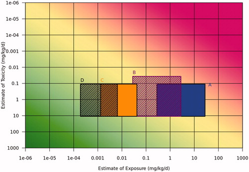
Table 9. Comparison of Tier 0 exposure estimates.

Exposure scenarios	Exposure estimates (mg/kg/day)
Adult workers	28
Child camper (Consumer)	2.79
Adult community resident via drinking water and fish ingestion, respectively, based on deltamethrin’s water solubility	7.4 × 10^−5+7.4 × 10^−3=7.4 × 10^−3
Adult community resident based on banded intake fraction	1.9 × 10^−4 to 6.5 × 10^−3

The risk assessment matrix in Figure 5 illustrates that a higher tiered assessment may be necessary for refining the exposure estimates for adult workers and child campers (consumer), whereas the adult community resident indirect exposure via solubility is borderline for need of further refinement. The case study also demonstrates that a variety of approaches can be used within a tier, depending upon available data. In this case, the look-up tables were found to provide quick estimates for direct and indirect contact scenarios, while a published point of departure (POD) for oral hazard was used for the toxicity estimate.

3.6. Tier 1 deterministic exposure assessment

To refine the exposure assessment in Tier 1, the adult worker scenario was modified using the information in Table 10. The Tier 1 assessment may be further informed with a WHO document on treating bed nets with deltamethrin to protect against malaria, “A generic risk assessment model for insecticide treatment and subsequent use of mosquito nets” (WHO 2004). Values from the WHO (2004) report are listed in Table 11.

Table 10. Tier 1 worker scenario refinements.

Parameters	Value
Hours spent transferring from large container to tank (hr)	15 min–1 h
Actual time workers might contact solution in dipping tank (hrs)	15 min–1 h
Deltamethrin concentration in plastic container (wt %)	5–25
Deltamethrin concentration in dipping tank (wt %)	No more than 1
Wearing protective gloves	Yes

Table 11. Reference values from WHO (2004) generic risk assessment.

Parameter	Value
Target dose (deltamethrin) on bed net (mg/m^2)	25
Sleeping inhalation rate (m^3/hr)	0.3
30% body surface area touching net while sleeping (m^2)	0.133
Hours under bed net (hr)	10
Child days at camp (days)	14*

* Given in the problem statement.

In addition to these refinements, the dermal absorption factor value of 5% from EPA Pyrethroid Cumulative Risk Assessment (U.S. EPA 2011b) can be used to further refine the exposure estimate. Refinement based upon dermal absorption is appropriate for this example, as the hazard benchmark represents an internal dose derived from an oral exposure study. If the hazard benchmark was based on external dermal exposure without conversion to absorbed dose, it would need to be compared to an external dermal exposure value and absorption would not be a consideration.

3.6.1. Adult worker tier 1 exposure estimate

The ECETOC TRA worker model was applied using the assumptions in Table 10 (1-h exposure time/day, <5 wt% final concentration in dipping tank) and a conservative protection factor of 10 was selected for wearing chemical protective gloves. For transfer (PROC 8a), dermal exposure is 0.83 mg/kg/day (with chemical protective gloves) and inhalation exposure is 0.032 mg/kg/day. For dipping (PROC 13), dermal exposure is 0.27 mg/kg/day (with chemical protective gloves) and inhalation exposure is 0.011 mg/kg/day. The combined worker exposure estimate for both activities (transfer and dipping) with 5% dermal absorption is (0.83 + 0.27) × 0.05 mg/kg/day + (0.032 + 0.011) mg/kg/day =0.098 mg/kg/day. Thus, the final worker Tier 1 exposure estimate is 0.098 mg/kg/day.

3.6.2. Child camper (consumer) tier 1 exposure estimate

The WHO (2004) default values used in this analysis are presented in Table 11. The surface area of body in contact with a net is 30%, which for children is 0.133, and the recommended insecticide loading on the bed nets is 25 mg/m². The amount of compound available for transfer from the net to the skin was used to estimate exposure. The WHO report indicates that 2.5% of the insecticide is dislodgeable from the net to skin. A 5% dermal absorption parameter was used based on EPA Pyrethroid Cumulative Risk Assessment (U.S. EPA 2011b). Taking these assumptions into account, the dermal exposure for child is 1 × 10⁻⁴ mg/kg/day.

Oral exposure via hand to mouth transfer was considered a relevant exposure pathway for children. The WHO (2004) report assumes that 10% of the amount transferred to the hand is then transferred to the mouth and is available for oral ingestion. The same parameters such as transfer coefficient based on dislodgeable fraction and insecticide loading were then applied. The WHO (2004) report lists the hand surface area for a child as 0.009 m². With these considerations, the oral exposure for child is 2 × 10⁻⁵ mg/kg/day. Oral exposure is considerably less than dermal exposure and thus does not significantly impact the overall exposure for children in this case.

3.6.3. Adult community resident tier 1 exposure estimate

For exposure to an adult community resident via the environment, the USEtox-specific intake fractions, based on similar but extended set of EPI Suite chemical properties, were applied for deltamethrin, yielding intake fractions for inhalation, fish and nonfish ingestion of 2.3 × 10⁻⁵, 9.2 × 10⁻⁵ and 2.7 × 10⁻⁵, respectively, a factor 20 lower than the banded iF determined in Tier 0. This reduced the Tier 1 exposures to a range of 3.6 × 10⁻⁶ to 1.2 × 10⁻⁴ mg/kg/day without and with accounting for variability characterized by the SV factors and HC factors (Table 6b).

The Tier 0 exposure assessment results fall orders of magnitude above the WHO (2004) screening estimates for exposures associated with dipping bednets in deltamethrin or sleeping on treated bednets. The Tier 1 estimates in this document are on a similar order of magnitude for adults and an order of magnitude lower for children. These differences reflect different parameters and data sources chosen in refinement, for example the WHO (2004) assessment uses a default of 10% dermal uptake, whereas the analysis here used a 5% dermal uptake value based upon data specific to deltamethrin.

3.7. Risk assessment and conclusions for Tier 1

The Tier 1 exposure estimates, summarized in Table 12, were plotted with the same POD oral hazard estimate and toxicity uncertainties from Tier 0, in the risk assessment matrix (Figure 6). The same toxicity benchmark was used for Tier 0 and Tier 1 to better demonstrate the effect of refining the exposure component. Since the exposure assessment has been refined based on the detailed information provided, a 30x uncertainty was assumed for the adult worker and child camper (consumer) exposures for the illustrative purpose of this example, with the estimated exposure as the midpoint in the range. The risk matrix indicates the adequate safety factors have been achieved for all three exposure scenarios. In this example there is no need to proceed on to higher tiers.

Figure 6. Tier 1 risk assessment matrix representing risk in the case study for (A) adult worker, (B) child camper (consumer), and (C) adult community resident exposed via the environment. The uncertainties represented by the boxes include 100× toxicity for the adult scenarios, 300× toxicity for child camper, and 30x exposure for adult worker and child camper. For adult community resident, the calculated range incorporated uncertainty.

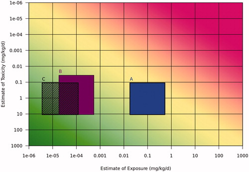
Table 12. Results of Tier 1 exposure estimates.

Exposure scenario	Exposure estimates (mg/kg/day)
Adult worker	0.098
Child camper (consumer)	1 × 10^−4
Adult community resident	3.6 × 10^−6 to 1.2 × 10^−4

4. Conclusions

This work demonstrates key aspects of the RISK21 approach including the initial emphasis on problem formulation, maximizing use of available information and the emphasis on using exposure information early in the process to focus the assessment on information most useful for decision making. These results show that predictive models that use the concept of exposure banding, first pioneered in the occupational exposure arena, lend themselves to the development of exposure look-up tables for risk assessments. The exposure estimates obtained were sufficiently discriminatory to assign risk assessment priority, focus exposure data collection efforts and suggest substance eligibility for elimination from higher tier risk and/or exposure assessment. The exposure look-up tables provide value because they deliver rapid, screening-level exposure estimates for a wide range of substances and their applications with limited data knowledge or input. The Tier 0 approaches were discussed in detail and a hypothetical case study was presented to illustrate the entire process of tiered risk assessment using banding and the risk visualization tool. Employing this approach will foster more rapid, efficient, and transparent risk analyses than is encountered in current practice.

Declaration of interest

This publication was authored collectively by participants of the ILSI HESI Risk Assessment in the 21st Century (RISK21) Technical Committee’s Exposure Sub-Team, whose work is supported by HESI, a nonprofit institution whose mission is to collaboratively identify and help to resolve global health and environment challenges through the engagement of scientists from academia, government, industry, NGOs and other strategic partners. HESI receives funding and in-kind support from member companies and other nonindustry organizations to support projects. The employment affiliation of the authors is shown on the cover page. These individuals had the sole responsibility for the writing and content of the paper, with additional input provided by other participants of the RISK21 Technical Committee’s Exposure Sub-Team (see acknowledgments). The individual authors worked as professionals in preparing the paper and not as agents of their employers. The views expressed in this paper are those of the authors and do not necessarily represent the views or policies of the U.S. Environmental Protection Agency. Travel expenses were provided for academic and government committee participants to attend committee meetings, and they did not receive any other compensation. This work has been presented at numerous international meetings, workshops and symposia to scientists and regulators from academia, industry and government.

Supplemental material

Supplemental material for this article is available online here.

Table A1: Worker Exposure Banding Approach A Step 1 Results

Table A2: Worker Exposure Banding Approach A Step 2 Results

Table A3: Worker Exposure Banding Approach A Step 3 Results

Table A4: Worker Exposure Banding Approach B HIGH Priority for Risk Assessment Substances

Table A5: Worker Exposure Banding Approach B MEDIUM Priority for Risk Assessment Substances

Table A6: Worker Exposure Banding Approach B LOW Priority for Risk Assessment Substances

Table A7: Worker Exposure Banding Approach B Possible Elimination from Risk Assessment Substances

Table B1: ECETOC TRA v3 Exposure Estimates by Exposure Route for VP ≥ 10 Pa

Table B2: ECETOC TRA v3 Exposure Estimates by Exposure Route for VP 1 ≤ 10Pa

Table B3: ECETOC TRA v3 Exposure Estimates by Exposure Route for VP 0.1 ≤ 1 Pa

Table B4: ECETOC TRA v3 Exposure Estimates by Exposure Route for VP < 0.1Pa

Abbreviations
AC	=	article category
ART	=	advanced REACH tool
ChemSTEER	=	chemical screening tool for exposures and environmental releases
ECETOC	=	European Centre for Ecotoxicology and Toxicology of Chemicals
E-FAST	=	exposure and fate assessment screening tool
EGRET	=	ESIG GES risk and exposure tool
EPA	=	Environmental Protection Agency
EPI	=	estimation program interface
ESIG	=	European Solvents Industry Group
EUSES	=	European Union system for the evaluation of substances
EXAMS	=	exposure analysis modeling system
GES	=	generic exposure scenario
HESI	=	Health and Environmental Sciences Institute
iF	=	intake fraction
ILSI	=	International Life Sciences Institute
LT	=	long term
MOE	=	margin of exposure
MW	=	molecular weight
NLM	=	National Library of Medicine
OECD	=	Organization for Economic Cooperation and Development
OEL	=	occupational exposure limit
PC	=	product category
POD	=	point of departure
PROC	=	process category
PRZM	=	pesticide root zone model
QSAR	=	quantitative structure–activity relationship
RAIDAR	=	risk assessment, identification and ranking model
RCR	=	risk characterization ratios
REACH	=	registration, evaluation, authorization, and restrictions of chemicals
RISK21	=	risk assessment in the twenty-first century
SCI-GROW	=	screening concentration in ground water
SETAC	=	Society of Environmental Toxicology and Chemistry
SHEDS-HT	=	stochastic human exposure and dose simulation-high throughput
SDWIS	=	safe drinking water information system
SPIN	=	substances in preparations in the Nordic countries
SRC	=	Syracuse Research Corporation
ST	=	short term
TRA	=	targeted risk assessment
TTC	=	threshold of toxicological concern
UNEP	=	United Nations Environment Program
USDA	=	U.S. Department of Agriculture
VP	=	vapor pressure
WHO	=	World Health Organization

Acknowledgements

The authors gratefully acknowledge the government, academic and industry scientists of the HESI RISK21 Technical Committee for their contributions to this work. (For a full list of RISK21 participants, see http://www.risk21.org). The authors also gratefully acknowledge the comments of four reviewers who were selected by the Editor and anonymous to the authors. The comments were helpful in revising the manuscript and improving its clarity.

References

- Albert RE. 1994. Carcinogen risk assessment in the U.S. Environmental Protection Agency. Crit Rev Toxicol. 24:75–85.
- Albert RE, Train RE, Anderson E. 1977. Rationale developed by the Environmental Protection Agency for the assessment of carcinogenic risks. J Natl Cancer Inst. 58:1537–1541.
- Apte JS, Bombrun E, Marshall JD, Nazaroff WW. 2012. Global intraurban intake fractions for primary air pollutants from vehicles and other distributed sources. Environ Sci Technol. 46:3415–3423.
- Arnot JA, Brown TN, Wania F, Breivik K, McLachlan MS. 2012. Prioritizing chemicals and data requirements for screening-level exposure and risk assessment. Environ Health Perspect. 120:1565–1570.
- Arnot JA, Mackay D, Webster E, Southwood JM. 2006. Screening level risk assessment model for chemical fate and effects in the environment. Environ Sci Technol. 40:2316–2323.
- Barlow S. 2005. Threshold of Toxicological Concern (TTC) – a tool for assessing substances of unknown toxicity present at low levels in the diet. ILSI Europe Concise Monographs Series. 2005:1–31.
- Bennett DH, McKone TE, Evans JS, Nazaroff WW, Margni MD, Jolliet O, Smith KR. 2002. Defining intake fraction. Environ Sci Technol. 36:206A–211A.
- Cook WA. 1969. Problems of setting occupational exposure standards– background. Arch Environ Health. 19:272–276.
- Devine JM. 1993. Occupational and consumer exposure assessments Annex 1: Approaches for developing screening quality estimates of occupational exposure used by the US EPA’s OPPT and their applicability to the OECD SIDS programme. In OECD Environment Monograph No. 70: [OCDE/GD(93)128]. Paris: OECD.
- Doe JE, Lander DR, Doerrer NG, Heard N, Hines RN, Lowit AB, Pastoor T, Phillips RD, Sargent D, Sherman JH, et al. 2016. Use of the RISK21 roadmap and matrix: human health risk assessment of the use of a pyrethroid in bed netting. Crit Rev Toxicol. 46:54–73.
- ECETOC. 2004. Targeted Risk Assessment, Technical Report No. 93, European Centre for Ecotoxicology and Toxicology of Chemicals. Brussels
- ECETOC TRA. 2012. ECETOC TRA version 3: Background and Rationale for the Improvements.
- ECETOC TRA. 2014. Addendum to TR114: Technical Basis for the TRA v3.1.
- ECHA. 2010. ECHA Guidance on information requirements and chemical safety assessment, R.12: Use Descriptor System.
- ECHA. 2012a. Guidance on information requirements and chemical safety assessment, Chapter R.14: Occupational exposure estimation. Helsinki, Finland.
- ECHA. 2012b. Guidance on information requirements and chemical safety assessment Chapter R.15: consumer exposure estimation.
- ECHA. 2012c. Guidance on information requirements and chemical safety assessment Chapter R.16: environmental exposure estimation.
- ECHA. 2013. Guidance on information requirements and Chemical Safety Assessment Chapter R.7a: Endpoint specific guidance. Helsinki, Finland.
- Egeghy PP, Judson R, Gangwal S, Mosher S, Smith D, Vail J, Cohen Hubal EA. 2012. The exposure data landscape for manufactured chemicals. Sci Total Environ. 414:159–166.
- Embry MR, Bachman AN, Bell DR, Boobis AR, Cohen SM, Dellarco M, Dewhurst IC, Doerrer NG, Hines RN, Moretto A, et al. 2014. Risk assessment in the 21st century: roadmap and matrix. Crit Rev Toxicol. 44:6–16.
- Hauschild MZ, Huijbregts M, Jolliet O, MacLeod M, Margni M, van de Meent D, Rosenbaum RK, McKone TE. 2008. Building a model based on scientific consensus for Life Cycle Impact Assessment of chemicals: the search for harmony and parsimony. Environ Sci Technol. 42:7032–7037.
- Henderson AD, Hauschild MZ, Van de Meent D, Huijbregts MAJ, Larsen HF, Margni M, McKone TE, Payet J, Rosenbaum RK, Jolliet O. 2011. USEtox fate and ecotoxicity factors for comparative assessment of toxic emissions in life cycle analysis: Sensitivity to key chemical properties. Int J Life Cycle Ass. 16:701–709.
- Mitchell J, Pabon N, Collier ZA, Egeghy PP, Cohen-Hubal E, Linkov I, Vallero DA. 2013. A decision analytic approach to exposure-based chemical prioritization. PLoS One. 8:e70911.
- Money CD. 2003. European experiences in the development of approaches for the successful control of workplace health risks. Ann Occup Hyg. 47:533–540.
- Munro IC, Ford RA, Kennepohl E, Sprenger JG. 1996. Correlation of structural class with no-observed-effect levels: a proposal for establishing a threshold of concern. Food Chem Toxicol. 34:829–867.
- NAS. 1983. Risk assessment in the federal government: managing the process. Washington, DC: National Academy Press
- OECD. 1993. Occupational and Consumer Exposure Assessments. Environment Monograph No 70.
- Pastoor TP, Bachman AN, Bell DR, Cohen SM, Dellarco M, Dewhurst IC, Doe JE, Doerrer NG, Embry MR, Hines RN, et al. 2014. A 21st century roadmap for human health risk assessment. Crit Rev Toxicol. 44:1–5.
- Pennington DW, Margni M, Amman C, Jolliet O. 2005. Multimedia fate and human intake modeling: spatial versus non-spatial insights for chemical emissions in Western Europe. Environ Sci Technol. 39:1119–1128.
- Rosenbaum RK, Bachmann TM, Gold LS, Huijbregts MAJ, Jolliet O, Juraske R, Koehler A, Larsen HF, MacLeod M, Margni MD, et al. 2008. USEtox – the UNEP-SETAC toxicity model: recommended characterization factors for human toxicity and freshwater ecotoxicicty in life cycle impact assessment. Int J Life Cycle Ass. 13:532–546.
- Ruckelshaus WD. 1983. Science, risk, and public policy. Science. 221:1026–1028.
- Russell M, Gruber M. 1987. Risk assessment in environmental policy-making. Science. 236:286–290.
- Shin HM, Ernstoff A, Arnot JA, Wetmore BA, Csiszar SA, Fantke P, Zhang X, McKone TE, Jolliet O, Bennett DH. 2015. Risk-based high-throughput chemical screening and prioritization using exposure models and in vitro bioactivity assays. Environ Sci Technol. 49:6760–6771.
- Stara JF, Kello D, Durkin P. 1980. Human health hazards associated with chemical contamination of aquatic environment. Environ Health Perspect. 34:145–158.
- U.S. EPA. 1986. Guidelines for estimating exposures. 51 FR 34042-34054.
- U.S. EPA. 1992. Guidelines for exposure assessment. U S Environmental Protection Agency risk assessment forum. Washington, D.C., EPA/600/Z-92/001.
- U.S. EPA. 2007. Pesticides industry sales and usage. 2006 and 2007 market estimates. In United States Environmental Protection Agency Office of Chemical Safety and Pollution Prevention. (7503P) EPA 733-R-11-001.
- U.S. EPA. 2011. U.S. Environmental Protection Agency (EPA) Exposure factors handbook, September 2011.
- U.S. EPA. 2011a. U.S. Environmental Protection Agency Estimation program interface (EPI) suite(EPI SuiteTM 4.10), 2000–2011.
- U.S. EPA. 2011b. U.S. Environmental Protection Agency (EPA) Cumulative pyrethroid risk assessment, October 2011.
- U.S. EPA. 2013. Next generation risk assessment: incorporation of recent advances in molecular, computational, and systems biology (external review draft), EPA/600/R-13/214A. In U.S. Environmental Protection Agency. Washington, DC.
- U.S. EPA. 2015. Human Health Ambient Water Quality Criteria: 2015 Update. Office of Water, EPA 820-F-15-001.
- Upton AC. 1988. Carcinogenic risk assessment in proper perspective. Toxicol Ind Health. 4:443–452.
- Verdonck FA, Boeije G, Vandenberghe V, Comber M, de Wolf W, Feijtel T, Holt M, Koch V, Lecloux A, Siebel-Sauer A, Vanrolleghem PA. 2005. A rule-based screening environmental risk assessment tool derived from EUSES. Chemosphere. 58:1169–1176.
- Vink SR, Mikkers J, Bouwman T, Marquart H, Kroese ED. 2010. Use of read-across and tiered exposure assessment in risk assessment under REACH – A case study on a phase-in substance. Regul Toxicol Pharm. 58:64–71.
- Wambaugh JF, Setzer RW, Reif DM, Gangwal S, Mitchell-Blackwood J, Arnot JA, Joliet O, Frame A, Rabinowitz JR, Knudsen TB, et al. 2013. High throughput models for exposure-based chemical prioritization in the ExpoCast project. Environ Sci Technol. 47:8479–8488.
- WHO. 1990. International programme on chemical safety. Environmental health criteria 97. Deltamethrin. World Health Organization Geneva. Available from: http://www.inchem.org/documents/ehc/ehc/ehc97.htm.
- WHO. 2004. A generic risk assessment model for insecticide treatment and subsequent use of mosquito nets. In Organization TWH.
- WHO. 2009. Assessment of combined exposures to multiple chemicals: Report of a WHO/IPCS international workshop on aggregate/cumulative risk assessment, International Programme on Chemical Safety. Harmonization Project Document 7.
- Zaleski RT, Qian H, Zelenka MP, George-Ares A, Money C. 2014. European solvent industry group generic exposure scenario risk and exposure tool. J Expo Sci Environ Epidemiol. 24:27–35.