3D Pharmacophore, hierarchical methods, and 5-HT₄ receptor binding data

Abstract

5-Hydroxytryptamine subtype-4 (5-HT₄) receptors have stimulated considerable interest amongst scientists and clinicians owing to their importance in neurophysiology and potential as therapeutic targets. A comparative analysis of hierarchical methods applied to data from one thousand 5-HT₄ receptor–ligand binding interactions was carried out. The chemical structures were described as chemical and pharmacophore fingerprints. The definitions of indices, related to the quality of the hierarchies in being able to distinguish between active and inactive compounds, revealed two interesting hierarchies with the Unity (1 active cluster) and pharmacophore fingerprints (4 active clusters). The results of this study also showed the importance of correct choice of metrics as well as the effectiveness of a new alternative of the Ward clustering algorithm named Energy (Minimum E-Distance method). In parallel, the relationship between these classifications and a previously defined 3D 5-HT₄ antagonist pharmacophore was established.

• 5-HT4
• antagonists
• pharmacophore
• clustering
• similarity

Introduction

In the last decade, much effort has been directed towards understanding the functions [1] of the various receptor subtypes of the neurotransmitter 5-hydroxytryptamine (5-HT; also known as serotonin). Amongst the 5-HT receptor subtypes, special attention has been paid to the most recently discovered ones, i.e. 5-HT₄, 5-HT₅, 5-HT₆ and 5-HT₇ 23456, all linked to stimulation of cAMP production. The 5-HT₄ receptor has generated the most interest [7] because of its importance in neurophysiology. Indeed, 5-HT₄ receptors have been demonstrated to modulate the release of neurotransmitters from various neuronal populations in the central nervous system, including basalocortical cholinergic [8,9], striatal dopaminergic [10,11] and hippocampal serotoninergic [12] cells. Moreover, 5-HT₄ receptors have been implicated in cognitive performance 1314151617, leading to the proposition that they could be targets for treatment of the cognitive deficits associated with Alzheimer's disease.

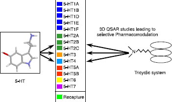
Our project began with the implementation of a screening platform related to 5-HT ligands (ATBI program). Design, synthesis, and biological evaluation of chemical compounds directed towards 5-HT₄, 5-HT_5A, 5-HT₆ and 5-HT₇ receptors are the initial objectives of this research program. The first phase was to study pharmacomodulation of a basic skeleton formed by an aromatic system bearing various substituents, and particularly an aminoalkyl chain (Figure 1).

Figure 1 General representation of the pharmacomodulation program.

The definition and comparison of pharmacophores for both 5-HT₃ receptor partial agonists [18] (Figure 2) and 5-HT₄ receptor antagonists (Figure 3) led to the design of new 5-HT₄ antagonists corresponding to selective compounds 1 and 2 (Scheme 1) [19,20].

Figure 2 5-HT₃ partial agonist pharmacophore.

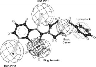
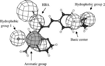
Figure 3 5-HT₄ antagonist pharmacophore.

Scheme 1 Structures of compounds 1 and 2.

The characteristics associated with 5-HT₄ ligands seem to be well-defined by this pharmacophore. Through our own work and through external collaborations, many other derivatives were tested against this receptor, generating 5-HT₄ receptor binding data for one thousand ligand–receptor complexes. This article provides an overview of these 5-HT₄ data, in terms of agreement with the 3D pharmacophore, similarities between invidious, and classification into chemical families. This last approach requires a comparison of the derivatives using a specific metric based on chemical descriptors and the application of clustering algorithms [21].

Materials and methods

Dataset

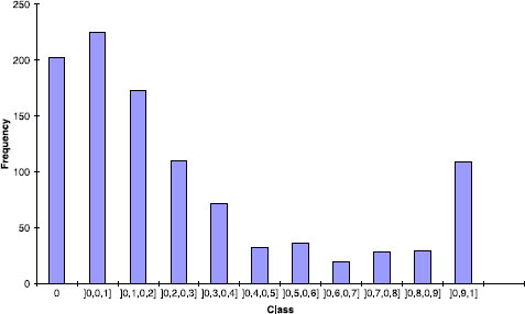
Percentage inhibition at two concentrations, 10^{− 6} M and 10^{− 8} M was determined. For the binding data recorded at 10^{− 6} M (Figure 4), the dataset was separated into three groups corresponding to active (percentage of inhibition ≥ 70%), intermediate (percentage of inhibition between 40% and 70%) and inactive derivatives.

Figure 4 Frequencies vs Class (%/100) associated with the percentage of inhibition at 10^{− 6}M.

The diversity of this data set was estimated by calculating dissimilarities between the different compounds based on the Unity fingerprint and Tanimoto coefficient (vide infra). The average and the density dissimilarity values for the nearest (ANN), farthest (AFN) and all neighbours (OAN) of each derivative were determined (Table I).

Table I.  Dataset dissimilarity values.

Dataset/Dataset	ANN	AFN	OAN
Overall/Overall	0.10	0.87	0.68
Actives/Inactives	0.42	0.80	0.67
Actives/Actives	0.06	0.76	0.46
Inactives/Inactives	0.12	0.87	0.70

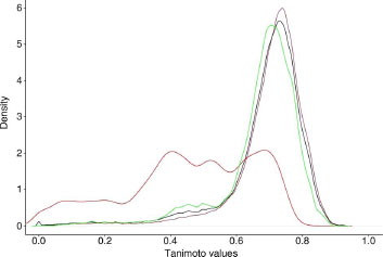
With a value around 0.5 (OAN) for the active compounds, these derivatives are more similar to one another compared to the overall dataset (0.7 for OAN). The graph (Figure 5) describing the density dissimilarity values clearly shows the particular range of dissimilarity values for the active compounds (red curve).

Figure 5 Overall Density Neighbors density representation. (black: overall; green: actives-inactives; red: actives-actives; brown: inactives-inactives).

3D pharmacophore and conformations

To test the 3D agreement of the different compounds towards our previous 3D 5-HT₄ antagonist pharmacophore (see Figure 3), a quasi-exhaustive conformational search was done for each compound (Fast method with Catalyst software). The maximum energy range between the conformers, and the maximum number of conformers for each compound were fixed at 20 kcal/mol and 250 (default values), respectively. In this study, a compound was considered as being in agreement with the 3D pharmacophore if it could fit all the pharmacophoric features whatever the value of the fit (fit value >0).

Fingerprints

Three classes of fingerprint descriptors were considered: hashed fingerprints, hybrid fingerprints (hashed and structural keys), and pharmacophore fingerprints. The first two encode chemical information in terms of bit strings. Pharmacophore fingerprints encode chemical features corresponding to atom types, in two ways: integer values for pharmacophore fingerprints and real values for fuzzy pharmacophore fingerprints.

JChem hashed fingerprints [22]

These fingerprints are generated by enumerating all cycles and linear paths up to a given number of bonds (maximum length of linear path) and hashing each of them into a fixed bit string (fingerprint length). The bit string generated depends on the number of bonds, the number of bits set (maximum pattern length), the length of the bit string, and the hashing function. Each of these parameters, except the fixed hashing function, has been optimised. By following criteria based on the notion that an optimum fingerprint must have a maximum darkness (percentage of bit 1 in the fingerprint) lower than 80% and an average darkness around 40%, the fingerprint length, the maximum linear path length, and the number of bits for each feature were chosen to be 1024, 7, and 3, respectively. A maximum darkness of 70.6% and an average darkness of 45.3% were obtained in this case.

Unity hybrid fingerprint [23]

This fingerprint corresponds to the analysis of length 2 through 6 fragments, the encoding of atom and bond types, and a fragment-based screen generation for heteroatoms and phenyl rings. Unity fingerprints represent each compound through a 988-dimensional bit string.

2-D atom-based pharmacophore fingerprints [22]

The interest of pharmacophoric fingerprints is logical by considering our previous data on 3D pharmacophore. Potential pharmacophoric point pairs (PPP) [24] were calculated. The following features were defined and applied for each atom: hydrogen bond acceptor/donor, hydrophobicity, aromaticity, and whether cationic or anionic. In this representation, each pattern of the fingerprint corresponds to the shortest path between two nodes (atoms/features) of the chemical graph. Starting from a distance between 1 and 10, the 210 fingerprint length encodes the number of times a pattern was found (integer values).

Fuzzy 2-D pharmacophore fingerprints [22]

The algorithm uses a smoothing factor to modulate the previous 2D atom-based pharmacophore fingerprints. The fuzzy pharmacophore led to a modulation of the initial distance between two features by applying a smoothing factor to the initial separation (n bonds). The default smoothing factor (0.7 in this case) led to the following multiplicative factors being applied to the initial value recorded for a distance of n bonds between two features: 0.15 (n − 1), 0.7 (n), and 0.15 (n + 1). This fingerprint has a 210 length with real values in this case.

Dissimilarity matrix for binary data

The function “fp.sim.matrix” of the R fingerprint package [25] was used with Euclidean, Tanimoto, modified Tanimoto, and Dice methods to obtain similarity values (C). From these similarity data, the dissimilarity coefficients (DC = 1 − C) were calculated to generate the dissimilarity matrix. In the following equations, a and d correspond to the co-occurrences between two fingerprints associated with “on” bits (value = 1) and “off” bits (value = 0), respectively. b corresponds to the number of “on” bits in one fingerprint and “off” bits in the second fingerprint (the reverse is true for c).

The Euclidean coefficient (E_B) [26] corresponds to the square root of the matching coefficient [27].

The Tanimoto coefficient (T) [28] corresponds to the well-known Jaccard-Tanimoto coefficient.

The modified Tanimoto (MT) [29] is a less size-biased coefficient compared to the Tanimoto coefficient. Indeed, the Tanimoto coefficient does not consider the “off” co-occurrences and it is also known to privilege small compounds in dissimilarity selection and large compounds in similarity selection [30].

The Dice coefficient (D) [31] is equivalent to the Tanimoto coefficient, except that a double weight is given to positive co-occurrences (a).

Dissimilarity matrix for continuous data

The function “dist” of the R cluster package [32] was used with Euclidean, Canberra, Maximum, and Binary methods.

The Euclidean distance (E_C) between compounds i and j corresponds to the classical equation where x_ik is the value of the N-vector associated with compound x_i at the k position.

The Canberra distance [33] (C) is a normalised distance. However, for its implementation in R (function “dist”), when the denominator is equal to zero, a value of 1 was considered in the final sum. This point was modified, and when the denominator is equal to zero, the value is omitted from the sum and treated as a missing value. With this modification, the results concerning the hierarchies were slightly improved.

The Maximum (M) distance considers only the maximum difference between two fingerprints.

Binary metric (B), transformed the fingerprints into a list of binary bits, so that the non-zero elements are “on” and the zero elements are “off”. Its definition leads to the dissimilarity form of the Tanimoto coefficient (B = 1 − T).

Clustering algorithms

Five hierarchical, agglomerative clustering methods were evaluated in this study. Four of them—Ward, Complete, Average and Single—are well-known. Energy is a new method [34] and has never been evaluated in chemical clustering. Single, complete and average linkage define the intercluster distances as the minimum, maximum, and average values, respectively, between two clusters 353637. Ward [38] and Energy [34] methods consider homogeneity and separability of the different clusters as a basis for the clustering. In contrast to the linkage method, these methods do not group together clusters with the smallest distances, but unify clusters such that the internal variation (dissimilarity values) does not increase too drastically. More precisely, during the clustering process, Ward minimises the increase, proportional to the square of the Euclidean distance, between cluster centres. In contrast, Energy, for the same approach, is based on the Euclidean distance. For this difference, previous data show that if the clusters are characterised by their means, Ward is a good choice; however, if the clusters are characterised by their distributions, then Energy is better [34].

Effectiveness

In the literature, three methods are popular to measure the effectiveness of the clustering process. The first one compares the final result (hierarchy) to a reference 394041. The second analyses the capacity of a clustering process to predict a molecular property [41,42]. The third method evaluates the separation between active and inactive compounds during the clustering process [24,43,44].

For the first method, no clustering reference corresponding to our dataset is present and a manual determination, based on the structures, will bias the comparison. For the second method, if the similarity techniques are based on the argument that similar compounds present the same biological activity, then the reciprocity is not available for inactive compounds. So, these methods were discarded and only the third method was kept. Brown et al. [24] defined an active cluster as having at least one active compound (singletons were not considered). Their studies led to the definition of an index, named Pa, corresponding to the proportion of active compounds in the active clusters. However, with this definition, an active compound alone in a large inactive cluster led to an important decrease of Pa (see Figure 6).

Figure 6 Evolution of the different indexes as a function of clustering level (Unity fingerprint/Tanimoto/Energy). (Pa curve in red, QCI curve in green; QCI_W curve in blue).

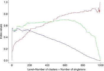
Thus, comparison of large clusters associated with a high level of clustering is biased by the presence of few active compounds in inactive clusters. Starting from this point and after several trials, we defined a new index based on a new definition of active clusters. In this study, an active cluster is a cluster (without considering the singletons) for which the percentage of active compounds is greater than the initial percentage of active compounds in the dataset (16.3%). From this definition, an optimal hierarchy must lead to a maximum number of active compounds in active clusters, a minimum number of inactive compounds in active clusters, a minimum number of active compounds in inactive clusters, and a minimum number of active singletons. With these points, an index (see Figure 6), named QCI for Quality Clustering Index, was defined with x corresponding to the number of active compounds in active clusters, y the number of inactive compounds in active clusters, z the number of active compounds in inactive clusters, and w the number of active singletons.

The next point concerns the optimal level, corresponding to the best separation between active and inactive compounds. Many indexes were proposed, but none seems to outperform any other [45]. In this study, we have considered that a small number of clusters must be privileged (low level of clustering). So, our index (QCI) was modulated by a multiplicative factor in relation to the level of clustering (weight of 1 for the first level to 1/1000 for the thousandth level), leading to the determination of a new index named QCI_W. The evolution of QCI_W values was followed, at each level, by calculating a Euclidean distance (QCI_WD) between the QCI_W curve and no classification (QCI_W = 0). Indeed, this last value (QCI_WD) allows the comparison of the different combinations (descriptor/metric/clustering algorithm) in terms of their capacities to separate active and inactive compounds during the overall clustering process.

Dendrogram

The function “A2RPlot.hclust” was used to build the representation, employing the e-distance (Energy) between merging clusters.

Results

Comparison of the hierarchy

The data were ranked as a function of QCI_WD values (see Table II).

Table II.  Classification of the hierarchies (the first twenty) as a function of QCI_WD values.

Fingerprint	Metric	Method	QCIWD
Pfp_JChem	Canberra	Energy	11.77
Pfp_JChem	Canberra	Ward	11.67
Pfp_JChem	Binary	Ward	11.54
Ufp_Unity	Tanimoto	Energy	11.35
Ufp_Unity	MT	Energy	11.33
Pfp_JChem	Binary	Energy	11.31
Ufp_Unity	Dice	Energy	11.30
Ufp_Unity	Euclidean	Energy	11.29
Ufp_Unity	MT	Ward	11.22
Cfp_JChem	MT	Energy	11.17
Pfp_JChem	Canberra	Complete	11.17
Cfp_JChem	Euclidean	Energy	11.17
Ufp_Unity	Tanimoto	Ward	11.17
Cfp_JChem	Euclidean	Ward	11.17
Fpfp_Jchem	Euclidean	Energy	11.14
Pfp_JChem	Euclidean	Energy	11.14
Cfp_JChem	Tanimoto	Energy	11.13
Ufp_Unity	Euclidean	Ward	11.12
Cfp_JChem	MT	Ward	11.08
Ufp_Unity	Dice	Ward	11.07

The best combinations were obtained with pharmacophore fingerprints/Canberra/Energy or Ward methods. Thus, pharmacophore fingerprints are able to differentiate very effectively between active and inactive compounds. This result was obtained with Canberra, for which the key point is that a difference between two observations associated with high values contributes less to the dissimilarity of two compounds. For instance, two compounds with 100 versus 99 observations for pharmacophoric pair feature A (a typical situation associated with hydrophobic–hydrophobic atoms separated by n bonds) and 2 versus 1 observations for pharmacophoric pair feature B (a situation associated with polar–polar atoms separated by n bonds), Canberra distances are equal to 0.005 for A and 0.33 for B whereas Euclidean distances are equivalent for the two compounds (values of 1). Moreover, if two compounds present, respectively, 10 and 0 observations of pharmacophoric pair feature A and 1 and 0 observations for pharmacophoric pair feature B, Canberra distances are equal to 1 whereas Euclidean distances are 10 for A and 1 for B. The same tendency is present with the binary metric. The highest values in our pharmacophore fingerprints correspond to hydrophobic features (this is classically the case). Our results show, that by decreasing the weight of these features, the clustering process is largely improved. Energy always gives better or equivalent results for the clustering process (Table III) compared to Ward. A clear explanation for this result is difficult at this time but we can suppose that our clusters are more efficiently characterised by their distributions instead of their means. The mean value is classically represented by a structure corresponding to a centroid. So the selection of this compound as a structure representative of a family or a comparison of the families based only on the centroid might not be so meaningful.

Table III.  Comparison as a function of QCI_WD values.

Fingerprint	Metric	Energy	Ward	Complete	Average	Single
Cfp_Jchem	Euclidean	11.17	11.17	10.60	10.26	9.40
Cfp_Jchem	Tanimoto	11.13	10.97	9.99	9.76	8.86
Cfp_Jchem	Dice	11.03	10.90	9.99	9.78	8.86
Cfp_Jchem	MT	11.17	11.08	10.39	9.99	9.07
Ufp_Unity	Euclidean	11.29	11.12	10.33	9.97	9.04
Ufp_Unity	Tanimoto	11.35	11.17	9.99	9.73	8.77
Ufp_Unity	Dice	11.30	11.07	9.99	9.73	8.77
Ufp_Unity	MT	11.33	11.22	9.94	9.77	8.83
Pfp_Jchem	Euclidean	11.14	11.05	10.50	10.23	6.18
Pfp_Jchem	Maximum	10.16	9.83	9.40	9.21	6.01
Pfp_Jchem	Canberra	11.77	11.67	11.17	10.68	7.44
Pfp_Jchem	Binary	11.31	11.54	10.62	10.20	7.33
Fpfp_Jchem	Euclidean	11.14	10.96	10.34	9.58	7.55
Fpfp_Jchem	Maximum	10.50	10.35	10.10	9.34	7.64
Fpfp_Jchem	Canberra	10.78	10.69	9.87	9.16	6.90
Fpfp_Jchem	Binary	8.78	7.88	7.42	6.69	5.77
Average		10.96	10.79	10.04	9.63	7.90
Standard Deviation		0.69	0.89	0.81	0.88	1.21

Unity fingerprints associated with Tanimoto or the modified Tanimoto (MT) coefficient and Energy method gave the most interesting results. The use of MT compared to Tanimoto did not improve the final result, indicating that the sizes of the structures in our dataset must be relatively homogeneous and have no influence on the final result.

For fuzzy pharmacophore, the results are less interesting than for the other fingerprints. The best results were obtained with Euclidean, Canberra or Maximum metrics associated with Energy. The binary metric was the worst performer. The concept of a smoothing factor is interesting but, in this case, a more specific metric should be defined for this descriptor.

Dendrogram

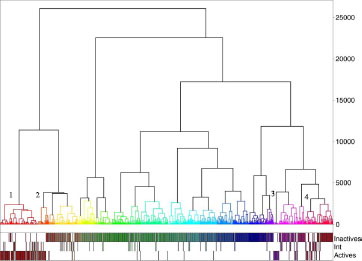
With “pharmacophore fingerprint/Canberra/Energy” and a level corresponding to the maximum value of QCI_W, four active clusters representing 88% of the active compounds of the overall dataset were obtained (see Figure 7). These four clusters include 72% of active compounds and 13% of inactive compounds, the remaining set corresponding to intermediate compounds. The dendrogram shows (see Figure 7), on the left side, a clear separation leading to the active clusters 1 (in red, left side) and 2 (orange, left side close to cluster 1). Cluster 1 represents 114 derivatives with 90 active compounds. Cluster 2 represents 33 derivatives with 22 active compounds. Cluster 3 represents 17 compounds with 16 active compounds. Cluster 4 represents 36 compounds with 15 active compounds.

Figure 7 Dendrogram associated corresponding to the best hierarchy based on pharmacophore fingerprint (Pfp_Jchem/Canberra/Energy). The numbers indicate the branches corresponding to active clusters (on the right of the number).

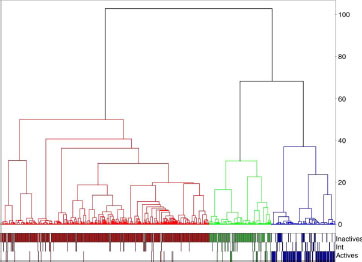
With the combination “Unity/Tanimoto/Energy” and a level corresponding to the maximum value of QCI_W, only one active cluster was obtained, including 66% of active compounds and 14% of intermediate compounds. The dendrogram clearly shows (see Figure 8) the rapid separation between active and inactive derivatives. Of the 1000 derivatives, the repartitions are 622 for cluster 1 (in red, inactive cluster), 186 for cluster 2 (in green, inactive cluster), and 192 for cluster 3 (in blue, active cluster).

Figure 8 Dendrogram corresponding to the best hierarchy based on chemical fingerprint (Ufp_Unity/Tanimoto/Energy).

3D pharmacophore

Analysis of the agreement between the conformations of the derivatives and our previous 3D pharmacophore (Figure 3) was carried out in parallel. The objective was to determine the quality of this 3D pharmacophore and also the relationships with the previous 2D analyses (fingerprints and clustering). If we considered the overall dataset, 25% of the derivatives fit the 3D pharmacophore and, of this set, 48% of the derivatives are active towards the 5-HT₄ receptor. By considering only active clusters defined by the previous selected clustering process (see Tables IV and V), 72% (+47% compared to the initial dataset) of the derivatives fit the 3D pharmacophore for the combination with pharmacophore fingerprint and 66% with Unity fingerprint. For inactive clusters, the great majority of compounds do not fit the 3D pharmacophore: 87% (+12% compared to the initial dataset) for pharmacophore fingerprint and 85% for Unity fingerprint. A more precise analysis of active clusters shows that, with pharmacophore fingerprint, 80% of the active compounds and 53% for the inactive compounds fit the pharmacophore (+28% compared to the initial dataset). For Unity fingerprint, the corresponding values were 81% of active compounds but only 37% of inactive compounds (+22% compared to the initial dataset). Therefore, the behaviours of pharmacophore fingerprint and 3D pharmacophore with respect to classification (active vs. inactive) in the active cluster are very close (closer than Unity fingerprint: 53% vs 37%). The same observation was made for inactive clusters, where 75% of active compounds do not fit the pharmacophore (compared to only 56% for Unity).

Table IV.  Line up of active and inactive clusters as a function of the activity and fit values.

			Number of compounds
Activity of clusters	Activity of compounds	Fit the pharmacophore	Pfp/Canberra/Energy	Unity/Tanimoto/Energy
Active	Active	Yes	114	103
		No	29	24
	Inactive	Yes	30	24
		No	27	41
Inactive	Active	Yes	5	16
		No	15	20
	Inactive	Yes	97	103
		No	683	669

Table V.  Percentage of compounds in active and inactive clusters in relation to fit towards the 3D pharmacophore.

			Percentage of compounds
Activity of clusters	Fit the pharmacophore	Compounds	Pfp/Canberra/Energy	Unity/Tanimoto/Energy
Active clusters	Yes	All	72 (+47)	66 (+41)
		Active	80 (+8)	81 (+9)
		Inactive	53 (+28)	37 (+22)
Inactive clusters	No	All	87 (+12)	85 (+10)
		Inactive	88 (+13)	87 (+12)
		Active	75 (+50)	56 (+31)

Overall, the 3D pharmacophore is very effective in being able to extract potential ligands from a database. Comparison of the clustering processes shows that 2D and 3D pharmacophores have similar behaviours for classification of derivatives.

Conclusion

This comparative analysis of different combinations associated with hierarchical clustering clearly shows the power of 2D chemical and pharmacophore fingerprints for efficiently classifying chemical derivatives in terms of molecular similarity and biological activity. We pointed out the importance of the metrics associated with each descriptor and particularly the Canberra approach for pharmacophore fingerprints. For the clustering algorithms, our study clearly demonstrates the effectiveness of a recent modification of the Ward method named Energy, irrespective of the fingerprint. Our study also illustrates the power of clustering approaches for rapidly obtaining an overview of the relationships between structures and biological data. However, it is necessary to apply the best available metric and global comparison of these metrics is actually carried out. Finally, the study underscores the quality of our previous 5-HT₄ antagonist pharmacophore in being able to extract potential 5-HT₄ ligands from a database.

Declaration of interest: The authors report no conflicts of interest. The authors alone are responsible for the content and writing of the paper.

References

- NM Barnes, and T Sharp. (1999). A review of central 5-HT receptors and their function. Neuropharmacology 38:1083–1152.
- J Bockaert, M Sebben, and A Dumuis. (1990). Pharmacological characterization of 5-hydroxytryptamine4(5-HT4) receptors positively coupled to adenylate cyclase in adult guinea pig hippocampal membranes: Effect of substituted benzamide derivatives. Mol Pharmacol 37:408–411.
- JL Plassat, U Boschert, N Amlaiky, and R Hen. (1992). The mouse 5HT5 receptor reveals a remarkable heterogeneity within the 5HT1D receptor family. EMBO J 11:4779–4786.
- FJ MonsmaJr, Y Shen, RP Ward, MW Hamblin, and DR Sibley. (1993). Cloning and expression of a novel serotonin receptor with high affinity for tricyclic psychotropic drugs. Mol Pharmacol 43:320–327.
- M Ruat, E Traiffort, JM Arrang, J Tardivel-Lacombe, J Diaz, R Leurs, and JC Schwartz. (1993). A novel rat serotonin (5-HT6) receptor: Molecular cloning, localization and stimulation of cAMP accumulation. Biochem Biophys Res Commun 193:268–276.
- M Ruat, E Traiffort, R Leurs, J Tardivel-Lacombe, J Diaz, JM Arrang, and JC Schwartz. (1993). Molecular cloning, characterization, and localization of a high-affinity serotonin receptor (5-HT7) activating cAMP formation. Proc Natl Acad Sci USA 90:8547–8551.
- RM Eglen. (1997). 5-Hydroxytryptamine (5-HT)4 receptors and central nervous system function: An update. Prog Drug Res 49:9–24.
- S Consolo, S Arnaboldi, S Giorgi, G Russi, and H Ladinsky. (1994). 5-HT4 receptor stimulation facilitates acetylcholine release in rat frontal cortex. Neuroreport 5:1230–1232.
- S Consolo, R Bertorelli, G Russi, M Zambelli, and H Ladinsky. (1994). Serotonergic facilitation of acetylcholine release in vivo from rat dorsal hippocampus via serotonin 5-HT3 receptors. J Neurochem 62:2254–2261.
- S Benloucif, MJ Keegan, and MP Galloway. (1993). Serotonin-facilitated dopamine release in vivo: Pharmacological characterization. J Pharmacol Exp Ther 265:373–377.
- PJ Karstaedt, H Kerasidis, JH Pincus, R Meloni, J Graham, and K Gale. (1994). Unilateral destruction of dopamine pathways increases ipsilateral striatal serotonin turnover in rats. Exp Neurol 126:25–30.
- DE Patterson, RD Cramer, AM Ferguson, RD Clark, and LE Weinberger. (1996). Neighborhood behavior: A useful concept for validation of “molecular diversity” descriptors. J Med Chem 39:3049–3059.
- DJ Fontana, SE Daniels, EH Wong, RD Clark, and RM Eglen. (1997). The effects of novel, selective 5-hydroxytryptamine (5-HT)4 receptor ligands in rat spatial navigation. Neuropharmacology 36:689–696.
- N Galeotti, C Ghelardini, and A Bartolini. (1998). Role of 5-HT4 receptors in the mouse passive avoidance test. J Pharmacol Exp Ther 286:1115–1121.
- S Letty, R Child, A Dumuis, A Pantaloni, J Bockaert, and G Rondouin. (1997). 5-HT4 receptors improve social olfactory memory in the rat. Neuropharmacology 36:681–687.
- E Marchetti, A Dumuis, J Bockaert, B Soumireu-Mourat, and FS Roman. (2000). Differential modulation of the 5-HT(4) receptor agonists and antagonist on rat learning and memory. Neuropharmacology 39:2017–2027.
- E Marchetti-Gauthier, FS Roman, A Dumuis, J Bockaert, and B Soumireu-Mourat. (1997). BIMU1 increases associative memory in rats by activating 5-HT4 receptors. Neuropharmacology 36:697–706.
- C Daveu, R Bureau, I Baglin, H Prunier, JC Lancelot, and S Rault. (1999). Definition of a pharmacophore for partial agonists of serotonin 5-HT3 receptors. J Chem Inf Comput Sci 39:362–369.
- A Hinschberger, S Butt, V Lelong, M Boulouard, A Dumuis, F Dauphin, R Bureau, B Pfeiffer, P Renard, and S Rault. (2003). New benzo[h][1,6]naphthyridine and azepino[3,2-c]quinoline derivatives as selective antagonists of 5-HT4 receptors: Binding profile and pharmacological characterization. J Med Chem 46:138–147.
- R Bureau, C Daveu, S Lemaitre, F Dauphin, H Landelle, JC Lancelot, and S Rault. (2002). Molecular design based on 3D-pharmacophore. Application to 5-HT4 receptor. J Chem Inf Comput Sci 42:962–967.
- M Halkidi, Y Batistakis, and M Vazirgiannis. (2001). On clustering validation techniques. JIIS 17:107–145.
- CHEMAXON., < http://www.chemaxon.com/jchem/doc/user/Screen.html>. Accessed.
- UNITY, Version 7.3, Tripos Inc., 2006., 1699 S. Hanley Road, St. Louis, MO 63144, USA.
- RD Brown, and YC Martin. (1996). Use of structure-activity data to compare structure-based clustering methods and descriptors for use in compound selection. J Chem Inf Comput Sci 36:572–584.
- R Project., < http://www.r-project.org/>. Accessed.
- J Gower, and P Legendre. (1986). Metric and euclidean properties of dissimilarity coefficients. J Classification 3:5–48.
- RR Sokal, and CD Michener. (1958). A statistical method for evaluating systematic relationships. Univ Kans Sci Bull 38:1409–1438.
- P Jaccard. (1901). Etude comparative de la distribution florale dans une portion des Alpes et du Jura. Bull Soc Vaudoise Sci Nat 37:547–579.
- M Fligner, JS Verducci, and PE Blower. (2002). A modification of the Jaccard-Tanimoto similarity index for diverse selection of chemical compounds using binary strings. Technometrics 44:110–119.
- JD Holliday, N Salim, M Whittle, and P Willett. (2003). Analysis and display of the size dependence of chemical similarity coefficients. J Chem Inf Comput Sci 43:819–828.
- LR Dice. (1945). Measures of the amount of ecologic association between species. Ecology 26:297–302.
- R Project. 2006., version 2.4.0.
- GN Lance, and WT Williams. (1967). Mixed-data classificatory programs. I. Agglomerative systems. Aus Comput J 1:15–20.
- GJ Szekely, and ML Rizzo. (2005). Hierarchical clustering via joint between-within distances: Extending Ward's minimum variance method. J Classification 22:151–183.
- K Florek, J Lukaszewiez, J Perkal, H Steinhaus, and S Zubrzchi. (1951). Sur la liaison et la division des points d'un ensemble fini. Colloquium Mathematicae 2:282–285.
- T Sorensen. (1948). A method of establishing groups of equal amplitude in plant society based on similarity of species content. K. Danske Vidensk Selsk 5:34.
- CA Glasbey. (1987). Complete linkage as a multiple stopping rule for single linkage clustering. J Classification 4:103–109.
- JH Ward. (1963). Hierarchical grouping to optimize an objective function. J Am Stat Assoc 58:236–244.
- JW Raymond, CJ Blankley, and P Willett. (2003). Comparison of chemical clustering methods using graph- and fingerprint-based similarity measures. J Mol Graph Modell 21:421–433.
- DJ Wild, and CJ Blankley. (2000). Comparison of 2D fingerprint types and hierarchy level selection methods for structural grouping using Ward's clustering. J Chem Inf Comput Sci 40:155–162.
- GW Adamson, and JA Bush. (1975). A comparison of the performance of some similarity and dissimilarity measures in the automatic classification of chemical structures. J Chem Inf Comput Sci 15:55–58.
- GM Downs, P Willett, and W Fisanick. (1994). Similarity searching and clustering of chemical-structure databases using molecular property data. J Chem Inf Comput Sci 34:1094–1102.
- H Matter, and T Poetter. (1999). Comparing 3D pharmacophore triplets and 2D fingerprints for selecting diverse compound subsets. J Chem Inf Comput Sci 39:1211–1225.
- H Matter. (1997). Selecting optimally diverse compounds from structure databases: A validation study of two-dimensional and three-dimensional molecular descriptors. J Med Chem 40:1219–1229.
- E Dimitriadou, S Dolnicar, and A Weingessel. (2002). An examination of indexes for determining the number of clusters in binary data sets. Psychometrika 67:137–159.