Semi-empirical model for timber truck speed profile and fuel consumption

ABSTRACT

This paper presents a semi-empirical model for driving speed simulation and estimation of energy use in timber trucks in Sweden. The model is composed of two parts; the first part takes as input road properties along a route and applies a kinematic model to simulate a driving pattern. The kinematic model contains parameters that are found statistically from large-scale recordings of CAN bus data from 21 timber trucks in 1 year. The second part applies a mechanistic model on the simulated speed profile to compute fuel use. The driving pattern simulator can predict the driving time and energy use with roughly the same variance as can be observed between different trucks and drivers following the same route. An average rolling resistance coefficient of 0.0068 was found from a coast-down study, but with substantial variation between vehicles.

KEYWORDS:

• Timber truck
• fuel consumption
• simulation
• driver behavior
• energy efficiency

Introduction

Road transportation of timber is responsible for a large fraction of forestry’s costs. The importance can be expected to grow following the transfer to a fossil-free economy and in view of rising energy prices. General route planning tools, like Google Maps and Open Street Routing Machine, are important instruments to reduce costs and the carbon footprint. Such tools include models for speed and energy use, but on an aggregated road section level based on statistics, which is too simplistic for heavy timber transportation where there is strong dependency between sections since driving must be adapted to events ahead. Moreover, statistics is often missing on low-volume roads.

Previous models for time and fuel estimation of timber transportation have largely worked on an integrated level where the vehicle and the driver are treated as one black box unit. Svenson and Fjeld (2016, 2017) make a direct link between road properties and weight and time and fuel consumption. A similar approach is made by Anttila et al. (2023), with focus on the Finnish road classes. Kärhä et al. (2023) present a statistical fuel consumption model for comparison of a 76-tonne with a 92-tonne timber truck combination. Anttila et al. (2022) present a fuel model based on machine learning applied on fleet management system (FMS) data. Their model considers several vehicle, road, and weather factors and can predict fuel use with a route-level average absolute error of 35%. They conclude that FMS data has inadequate resolution for an otherwise successful approach. An overview of earlier studies of the impact of road characteristics on truck operating speed and fuel consumption is presented by Svenson and Fjeld (2017).

Various models for driver behavior on the vehicle level, so-called microscopic traffic modeling, have been described in the literature. The model developed in this project is in spirit similar to CHIP-TRUCK (Simwanda et al. 2015) and SUMO (Simulation of Urban Mobility), described by Behrisch et al. (2011). The SUMO model has later been expanded in various ways, for instance with the influence of curves (Kharrazi et al. 2018). The novelty of the present model is, apart from the mathematical and statistical treatment based on large scale driving data, that it in contrast to most other behavior models focuses on heavy vehicles and particularly timber vehicles. Behavior models for heavy vehicles require more consideration of physical limitations than is the case for cars, for instance to treat hills and different gross weights realistically.

There exist several fuel consumption models for heavy vehicles. They vary in detail and purpose. The highest level of detail have mechanistic models such as VETO (Hammarström and Karlsson 1987) or VECTO (European commission 2019). They entail detailed models of the drivetrain and were primarily intended for environmental certification but have later found use for development of applications such as intelligent cruise control and gear shift algorithms. The accuracy of VECTO is stated to be 3% (European Commission 2018), although it is not completely clear what the figure refers to. Other models have lower resolution (HDM-3 (Watanatada et al. 1987), HDM-4 (Kerali 2004)) and are primarily intended for modeling on an infrastructure level.

Apart from routing, the models can be used to make ex-ante full cost analysis and CO₂ footprint estimations of transportation missions, which is useful for new price models that consider the physical properties of the individual transportation trips. The idea is that a good match between remuneration and actual costs simplifies the work of a transportation manager, who may be prompted to assign transportation missions to different haulers with equal profitability in mind, rather than logistic efficiency, if a price model based solely on distance is used. In the course of work in the project “Energy efficiency through a new model for transport business contracts,” financed by the Swedish Energy Agency, it was observed that existing models for time and energy use are either too focused on individual details, or too general for the application at hand. The aim of the present article is to fill this gap and to present real world values of some important technical parameters describing timber trucks. The work presents an effort to separate technical from human aspects, to develop a model that is robust to varying (and even extreme) conditions and that in the future can be expanded to account for electric or other alternative propulsion systems.

Materials and methods

Data collection

The models presented in this paper are of a semi-empiric nature. They are based on mathematical models derived from kinematical and physical relations and entail a set of free parameters. The parameters are determined statistically from a very large set of driving data recorded from the CAN bus of 21 vehicles during a follow-up study extending over 1 year. The vehicles varied with respect to engine power, number of axles, tire types and loader arrangement, as presented in Table 1. The project fleet composition was roughly the result of a “wish list” and is expected to reflect roughly Sweden’s timber truck fleet over the coming years. It is difficult to have sufficient turnout for a randomized selection of vehicles for a follow-up study of the kind made in this work. On the other hand, the models developed in the project are intrinsically not very dependent on a statistically representative test fleet.

Table 1. Test fleet composition. “Axles” refers to the number of axles on the truck and the trailer, respectively. In general, maximum allowed gross vehicle weight for combinations with 7, 8, and 9 axles are 64 tonnes, 70 tonnes, and 74 tonnes.

Vehicle	Truck	Model year	Power (kW)	Axles	Trailer tires	Loader
1	Volvo FH 64R	2018	552	3+4	dual	fixed
2	Scania R580b	2020	427	3+5	dual	fixed
3	Volvo FH13	2018	405	3+5	dual	fixed
4	Scania R580b	2018	427	3+4	dual	detachable
5	Volvo FH 64R	2019	405	3+4	dual	separate loader
6	Scania R580b	2019	427	3+4	dual	separate loader
7	Scania R580b	2018	427	4+4	single	separate loader
8	Scania R580b	2018	427	4+4	dual	separate loader
9	Volvo FH 64R	2018	405	3+5	dual	detachable
10	Volvo F16	2015	375	4+4	single	separate loader
11	Scania 650	2019	478	4+5	single	separate loader
12	Volvo FH16	2020	552	4+5	dual	separate loader
13	Scania 650	2019	478	4+5	single	detachable
14	Volvo FH16	2019	552	4+5	dual	separate loader
15	Scania 650	2018	478	4+5	dual	separate loader
16	Scania R580b	2018	427	3+4	dual	detachable
17	Scania R520b	2016	382	3+4	dual	detachable
18	Volvo FH13	2016	405	3+5	dual	detachable
19	Volvo FH16	2016	552	3+5	dual	detachable
20	Scania R730b	2021	537	4+5	dual	separate loader
21	Volvo FH16	2020	552	4+5	dual	detachable

In total, over 700,000 km of driving was recorded. CAN data was recorded using a data logger (Owasys 450) and a contactless CAN-bus reader installed in each vehicle. The data logger also contains a GNSS receiver for positioning. Data is buffered and uploaded to a server using the 4G mobile phone network when permitted by coverage. Apart from CAN data, information from the Swedish road database (NVDB) and vehicle weight information from Biometria¹ was used. A major part of the present work has been to implement algorithms for automatic data extraction, identification of different driving conditions and merging of the different data sources.

Installation and management of the logging equipment presented considerable challenges. There was some data loss during the project due to problems with the data loggers. Some of the vehicles spent time in workshops for repairs and one vehicle was wrecked in an accident.

The CAN bus on heavy vehicles is used for communication between different units of the engine management system and other systems, according to the J1939 protocol. Odometer and signals for speed and instantaneous fuel rate are available, but to ensure accuracy a calibration routine is necessary. Distance and speed are readily checked against the GNSS receiver and were generally found to be accurate within 1%. The fuel rate is more cumbersome (Wang et al. 2017). It is normally only possible to compare fueled volumes with the vehicle’s internal signal for accumulated fuel use. Fueling protocols for around 1 month (20–30 fillings) were collected and a correction factor determined. The average absolute error in the internal fuel signal was found to be 1.4% and the standard deviation 4.5%. The accuracy of station fuel meters is regularly checked by the authorities and must be within 0.5%, but the average error is 0.2%. The results underline the importance of a calibration procedure for any fuel consumption follow-up where different vehicles are compared.

The developed models have been evaluated against a test data set containing driving sequences of varying length to test their predictive power.

A two-part mechanistic model for time and energy use

Together with the physical properties of the vehicle and the route, the driver’s behavior determines time and energy use. The driver adjusts speed according to a range of factors where safety and economy are key considerations. The performance of the vehicle also imposes constraints on what behavior can physically be realized. In the end, the behavior is manifested as a speed profile along the driven route. From this speed profile the time consumption is immediately given. From the speed profile and external factors such as temperature, road grade, etc., the vehicle responds with a fuel consumption. The consumption is calculated using a physical model of the vehicle with speed profile and the external factors as input.

Driver behavior model

It is of course impossible to exactly predict the speed at each position for an individual vehicle since each driver is unique and reacts to a dynamic traffic situation. It is, however, possible to formulate a set of general behavior rules from big data sets of driving data in combination with physical and legal limitations. Applied on a route, these rules generate a kind of average behavior.

The model assumes that the driver at each instant tries to keep as high a speed as possible, with respect to all given constraints such as speed limit, curve radius, etc. On the one hand, there are constraints on how fast the vehicle can accelerate with respect to driver comfort, engine power and traction. On the other hand, the driver must always, with reasonable deceleration, be able to reduce speed to respect all speed constraints further ahead. “Reasonable” refers to comfort, safety, and economic driving.

Limitations

The presented behavior model is limited to the static part of the traffic situation. Most timber transportation takes place on low volume private roads or on rural public roads, where interaction with other vehicles is usually small. Congestion, duty to turn, overtaking slow vehicles, etc., are stochastic in their nature and must be handled statistically somehow, either as standard corrections per the road stretches at hand or through a more elaborate discrete-event simulation (Kitamura and Kuwahara 2006). This is beyond the scope of this work, although the simulation model presented can be used to analyze the individual effect of such events.

Kinematic description

Denote by $\mathit{x}$ the position of the vehicle along the road. This refers to the path length whether the road is curved or straight. We are searching for the maximum speed $v_{\mathit{max}}\left(\mathit{x}\right)$ that the vehicle can keep at each point $\mathit{x}$. Divide the road into discrete points $x_1,x_2,\dots ,x_N$ (with sufficient resolution for computational accuracy, 1.0 m having shown suitable) reached at times $t_1,t_2,\dots ,t_N.$ Then, $v_{\mathit{max}}\left(x_k\right)$ is determined by:

• the possibility to accelerate from $v_{\mathit{max}}\left(x_{\mathit{k}-1}\right)$ with respect to power, weight, road grade, driver comfort, etc.,

• speed limit at $x_k$,

• practical speed limits imposed by curve radius, road width, etc., and

• the possibility to slow down to $v_{\mathit{max}}\left(x_{\mathit{k}+1}\right)$, if lower than $v_{\mathit{max}}\left(x_k\right)$, with comfortable deceleration.

To first order (Equation 1(1) $x_k=\frac{{\mathit{a}}_{\mathit{k}-1}}{2}\mathrm{\Delta }{t}^2+v_{\mathit{k}-1}\mathrm{\Delta }\mathit{t}+x_{\mathit{k}-1,}$(1) )

(1) $x_k=\frac{{\mathit{a}}_{\mathit{k}-1}}{2}\mathrm{\Delta }{t}^2+v_{\mathit{k}-1}\mathrm{\Delta }\mathit{t}+x_{\mathit{k}-1,}$(1)

where $a_{\mathit{k}-1}$ and $v_{\mathit{k}-1}$ are acceleration and speed at $x_{\mathit{k}-1}$. $\mathrm{\Delta }\mathit{t}$ denotes the time to travel from $x_{\mathit{k}-1}$ to $x_k$. Together with the also first-order accurate relation $v_k=a_{\mathit{k}-1}\mathrm{\Delta }\mathit{t}+v_{\mathit{k}-1}$, this yields (Equation 2(2) $v_k^2=v_{k-1}^2+2\left(x_k-x_{\mathit{k}-1}\right)a_{\mathit{k}-1}.$(2) )

(2) $v_k^2=v_{k-1}^2+2\left(x_k-x_{\mathit{k}-1}\right)a_{\mathit{k}-1}.$(2)

The vehicle accelerates until any of the speed restrictions is reached. Acceleration is positive when speed is increasing, and negative for braking. Thus also (Equation 3(3) $v_k^2=v_{k+1}^2-2\left(x_{\mathit{k}+1}-x_k\right)a_k.$(3) ),

(3) $v_k^2=v_{k+1}^2-2\left(x_{\mathit{k}+1}-x_k\right)a_k.$(3)

Equations (2)(2) $v_k^2=v_{k-1}^2+2\left(x_k-x_{\mathit{k}-1}\right)a_{\mathit{k}-1}.$(2) and (3(3) $v_k^2=v_{k+1}^2-2\left(x_{\mathit{k}+1}-x_k\right)a_k.$(3) ) are nonlinear difference equations whose solutions are computed iteratively from initial and end values $v_1$ and $v_N$. To determine $v_{\mathit{max}}\left(x_k\right)$, a forward pass and a backward pass are required. In the forward pass, maximum speed $v^{\mathit{forw}}=v_k$ with respect to feasible acceleration is determined using Equation (2)(2) $v_k^2=v_{k-1}^2+2\left(x_k-x_{\mathit{k}-1}\right)a_{\mathit{k}-1}.$(2) . In the backward pass, Equation (3)(3) $v_k^2=v_{k+1}^2-2\left(x_{\mathit{k}+1}-x_k\right)a_k.$(3) gives maximum speed $v^{\mathit{back}}=v_k$ with respect to the need to be able to slow down with feasible deceleration, facing restrictions ahead. $v_{\mathit{max}}\left(x_k\right)$ is the smaller of the speeds from the two passes.

Pseudo code for simulation

In this section, an algorithm for the speed profile simulator is presented. Symbols according to Table 2 are used.

Table 2. Symbols used for the behavior model.

Symbol	Meaning	Typical values	Unit
$v^{\lim }$	Speed limit	8–22	ms^−1
$v^{\mathrm{curve}}$	Highest speed with respect to horizontal curvature. Determined statistically.	1.0–22	ms^−1
$v^{\mathrm{rdw}}$	Highest speed with respect to road width. Determined statistically.	5–22	ms^−1
$v^{\mathrm{vis}}$	Highest speed with respect to visibility.	variable	ms^−1
$v^{\mathrm{cls}}$	Highest speed with respect to road class. Determined statistically.	11–22	ms^−1
$a^{\max }$	Acceleration. Limited by engine power, speed, gross weight, road gradient, traction and driver comfort. Determined statistically but physically limited.	0.0–0.5 (Can be negative for steep climbs.)	ms^−2
$a^{\min }$	Deceleration. Mainly determined by economical driving. Determined statistically.	−0.6–0.0	ms^−2
$a^{\mathrm{lov}}$	Deceleration at sudden loss of visibility. Value according to Swedish Road Administration (2015).	−1.0	ms^−2
$a^{\mathrm{em}}$	Highest emergency deceleration. Value according to Swedish Road Administration (2015).	−2.0	ms^−2
$\mathit{S}$	Line of sight. Calculated.	>10	m
$\mathit{R}$	Curve radius. From NVDB.	>10	m

% Speed profile simulation from statistical behavior parameters

$v_N^{\mathrm{back}}:=\mathrm{end}\mathrm{speed}$ of driving sequence

$\mathbf{for}\mathit{k}:=\mathit{N}-1,\mathit{N}-2,\dots ,1\text{break}\mathrm{\Delta }\mathit{x}:=x_{\mathit{k}+1}-x_k$

Determine $a^{\min }$ from statistics.

$v_k^{\mathrm{back}}:=\text{break}\min \left(\sqrt{{\left(v_{k+1}^{\mathrm{b}\mathrm{ack}}\right)}^2-2\mathrm{\Delta }\mathit{x}{a}^{\min }\left(v_{k+1}^{\mathrm{back}}\right)},v^{\lim }\left(x_k\right),\text{break}{v}^{\mathrm{curve}}\left(x_k\right),v^{\mathrm{rdw}}\left(x_k\right),v^{\mathrm{cls}}\left(x_k\right)\right)$

end

$v_1^{\mathrm{forw}}:=\mathrm{initial}\mathrm{speed}$ of driving sequence

$\mathbf{for}\mathit{k}:=2,3,\dots ,\mathit{N}\text{break}\mathrm{\Delta }\mathit{x}:=x_k-x_{\mathit{k}-1}$

Determine $a^{\max }$ from statistics, physical limits, and visibility.

$v_k^{\mathrm{forw}}:=\text{break}\min \left(\sqrt{{\left(v_{k-1}^{\mathrm{f}\mathrm{orw}}\right)}^2+2\mathrm{\Delta }\mathit{x}{a}^{\max }\left(v_{k+1}^{\mathrm{forw}}\right)},v^{\lim }\left(x_k\right),\text{break}{v}^{\mathrm{curve}}\left(x_k\right),v^{\mathrm{rdw}}\left(x_k\right),v^{\mathrm{cls}}\left(x_k\right)\right)$

end

$\$\mathbf{for}\mathit{k}:=2,3,\dots ,\mathit{N}-1\text{break}{v}_{\max }\left(x_k\right)\mathit{\hspace{0.17em}}:=\min \left(v_k^{\mathrm{forw}},v_k^{\mathrm{back}}\right)$

end

The simulated speed profile is semi-empiric in the sense that it is computed from observed driving patterns, such as acceleration and deceleration as a function of speed, or maximum speed as a function of road width or curve radius. As the model uses parameters for observed vehicle speed profiles, it works whether the vehicle is driven manually or with the aid of intelligent cruise control. Since physical limits are always respected, extreme combinations of input parameters are handled without giving unreasonable output. Similar models have been presented e.g. by Yang et al. (2016) or Kharrazi et al. (2018). The present model differs from earlier work in that it employs kinematic/kinetic principles rather than purely statistical relations to model the combined effect of different factors.

Statistical determination of parameters

The CAN-data loggers produced 1 Hz resolved data on;

• Position and time

• Speed

• Brake application

• Gross weight from air suspension

In addition, data from the Swedish National Road database (NVDB) were added;

• Speed limit

• Road gradient

• Functional road class

• Road width

A standard approach for model parameter identification is to determine the set of parameters giving the best fit between model and measurements. This procedure is not always robust, though, and in particular if there are uncertainties in the input data. An alternative approach was therefore used in this project, where certain events, such acceleration or braking were isolated and analyzed separately.

Acceleration and deceleration behavior

Random events notwithstanding, most drivers appear to follow largely the same pattern for acceleration and deceleration. The former is initially limited by driver comfort. As speed is picked up, available power becomes limiting. The deceleration practice is an important part of eco-driving. When approaching, for instance, a crossing at highway speed, deceleration is initially low using engine braking or coasting. Eventually, as momentum is lost, the driver applies the foundation brakes, increasing deceleration.

The statistical determination of the braking behavior is done from identified sequences of deliberate deceleration. These were defined as $\ge 10$ s long sections of the speed profile for which speed was reduced by $\ge 10$ kmh⁻¹ and without positive power output from the engine (so that steep climbs are not identified as braking). A similar analysis was done for acceleration. The result is presented in Tables 3 and 4. The number of sequences was 211,000 for deceleration and 229,000 for acceleration.

Table 3. Deceleration depending on speed. Intervals in kmh⁻¹ and deceleration in ms⁻². (intervals do not include their right end point.)

Season	Speed interval
	0–<5	5–<15	15–<25	25–<35	35–<45	45–<55	55–<65	65–<75	75–<85	85–<95
	Loaded vehicle
winter	−0.32	−0.33	−0.38	−0.39	−0.32	−0.26	−0.22	−0.19	−0.15	−0.12
summer	−0.35	−0.41	−0.42	−0.45	−0.37	−0.29	−0.24	−0.20	−0.16	−0.13
	Unloaded vehicle
winter	−0.34	−0.39	−0.46	−0.52	−0.46	−0.38	−0.31	−0.26	−0.20	−0.15
summer	−0.37	−0.44	−0.48	−0.56	−0.52	−0.43	−0.35	−0.29	−0.22	−0.17

Table 4. Acceleration depending on speed. Intervals in kmh⁻¹ and acceleration in ms⁻² (intervals do not include their right end point.).

	Speed interval
	0–<5	5–<15	15–<25	25–<35	35–<45	45–<55	55–<65	65–<75	75–<85	85–<95
	Loaded vehicle
winter	0.31	0.26	0.29	0.29	0.25	0.21	0.18	0.16	0.13	0.12
summer	0.35	0.31	0.32	0.31	0.27	0.22	0.19	0.17	0.14	0.12
	Unloaded vehicle
winter	0.35	0.33	0.36	0.41	0.39	0.33	0.29	0.24	0.17	0.13
summer	0.40	0.39	0.38	0.44	0.43	0.37	0.33	0.28	0.19	0.13

Evidently, both deceleration and acceleration are lower when the vehicle is loaded and during wintertime.

Influence of horizontal curves

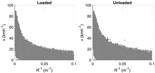
Curves impose a clear limit on speed with respect to comfort and safety. As suggested by the behavior model, there is no simple relation between speed and the diverse parameters at a single position along the route, but rather an implicit dependency on previous and later speeds. For any given curve radius, a spectrum of speeds will be observed since the driver has to respect speed limit, curves ahead or is simply under acceleration. From two-dimensional histograms showing observed speeds for different curvatures, it is possible to identify the maximum allowed speed for a certain curvature. Figure 1 shows the distribution of speeds for different curvature for one of the trucks during January – February. The number of observations in bins of size 1 kmh⁻¹ $\times$ 0.001 m⁻¹ have been counted, and only bins populated by at least 0.001 of the observation for each respective curvature are shown. The value 0.001 is somewhat arbitrary, but the result is not very sensitive to the choice. As expected, curve speed goes down as the curve radius decreases and speed is lower for loaded trucks than for unloaded trucks. For very low levels of curvature, there are virtually no observations of low speeds. This comes as no surprise since straight roads tend to be highways. There are also some artifacts stemming from noise in the GNSS-based computation of curvature.

Figure 1. Relationship between curvature and speed for one of the vehicles when loaded and unloaded.

Having computed the envelope of the histograms for all 21 vehicles, average curves were computed for summer and winter conditions (Figure 2). The curve-speed is lower during wintertime than summertime, but the difference is rather small. The graphs also show the curve-speed relationship calculated according to the formula (Equation 4(4) $\mathit{R}>\frac{v^2}{\left(0.28e^{-0.0346\mathit{v}}+\mathit{E}\right)\mathit{g}}$(4) ) formerly used by the Swedish Road Administration (2004).

Figure 2. Empirical relationship between curvature and maximum speed during winter and spring when loaded and unloaded. Also indicated is the dependency according to a formula used by the Swedish Road Administration (2004).

(4) $\mathit{R}>\frac{v^2}{\left(0.28e^{-0.0346\mathit{v}}+\mathit{E}\right)\mathit{g}}$(4)

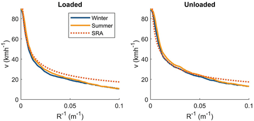
Here, $\mathit{v}$ is the speed in ms⁻¹, $\mathit{E}$ the crossfall in percent (0 for the curves in the graph), and $\mathit{g}$ the gravitational acceleration. The formula is useful for curves that are not too sharp, for which it overestimates speed.

Influence of road width

The influence of road width on maximum speed is determined using the same method as for curvature. The resulting averaged curves are shown in Figure 3.

Figure 3. Maximum speed depending on road width when loaded and unloaded.

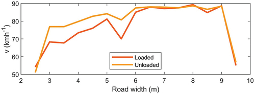
The tendency is clear: maximum speed is lower on narrow roads. However, fairly high speeds are observed also on narrow roads. Conversely, maximum speed seems to go down on roads of 5.5 m width and wider than 9 m. The explanation is that road width data from NVDB is not always reliable and seems to use default values where data is missing on roads of poor standard. This is particularly the case on the private road network and the reason why it was not fruitful to add a combined road width-curvature factor.

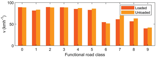
Functional road class

Swedish roads are classified on a scale 0–9 according to their role in the infrastructure. 0 is for highways and 7–9 for low volume roads. A connection between functional road class and maximum speed was made similarly as for other road properties. Figure 4 shows year averaged values for all vehicles. Only on private roads (class 7–9) is there an appreciable difference between the loaded and unloaded state.

Figure 4. Relationship between speed and functional road class when loaded and unloaded.

Line of sight

Visibility and the ability to stop facing unexpected obstacles are two important factors for safe driving. When comparing simulated and observed driving profiles without considering the line of sight, large differences often appear, especially on poor roads. It can be assumed that these are often due to limited visibility (uneven road surface may be another cause). In principle, the driver must be able to stop within the visible section of the road ahead. This cannot always be fulfilled in practice since the line of sight can change abruptly. In such cases, it is reasonable for the driver to settle for a more cautious braking (rather than a sudden stop) to better match speed to visibility. From the value of line of sight, maximum emergency deceleration and reasonably comfortable deceleration in case the speed is to high considering visibility, a heuristic rule can be formulated: If the speed exceeds $v^{\mathrm{vis}}=\sqrt{-2\mathit{S}{a}^{\mathrm{em}}}$, the highest speed permitting an emergency stop within distance $\mathit{S}$, braking with “reasonable” deceleration $a^{\mathrm{lov}}$ is initiated and continued as long as necessary. Only the forward pass is affected since it is hard to predict visibility changes ahead. NVDB lacks line of sight information. Instead, $\mathit{S}$ was calculated from the road geometry, topography, and width. The right-of-way also enters but data is again lacking, and a value must be assumed. On large roads of high standard, it can be presumed that all specifications are met, and that visibility is rarely a limiting factor. For low volume (mainly private) roads, one must rely on calculations based on existing information and assumptions.

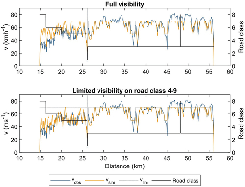
Figure 5 shows an example of one recorded and one simulated speed profile with and without consideration to visibility. The graphs also show the legal speed limit and the functional road class. It is apparent that on the narrow roads in the beginning of the route, the observed speed is kept down below what is possible with respect to speed limit, hills and curves. Adding the model for line of sight qualitatively improves the result, although a perfect match is not achieved. There are some cases of speeding in the recorded data.

Figure 5. Simulated speed profile and the influence of visibility.

Vehicle response model

VECTO can be applied on prescribed driving profiles from the driver model, but here we propose a model that is intermediate in complexity, essentially similar to Giannelli et al. (2005). The focus has been to determine and use values of some important parameters, mainly rolling resistance and air drag. The literature on these parameters is abundant, but reported values vary considerably, possibly due to varying equipment or experimental conditions.

Symbols according to Table 5 are used in the vehicle response model.

Table 5. Symbols used for the vehicle response model.

Symbol	Meaning	Typical values	Unit
$C_r$	Coefficient of rolling resistance	0.006	-
$C_d$	Coefficient of air drag	0.8	-
$F_{\mathit{rr}}$	Rolling resistance force	1–5	kN
$\mathit{A}$	Frontal area	10.4	m^2
$\mathit{N}$	Normal force	variable	N
$\mathit{m}$	Gross weight	17,000–74,000	kg
$m_{\mathrm{rot}}$	Rotating mass equivalent (depends on wheel number and type)	1,550–1,950	kg
$m_{\mathrm{eff}}=\mathit{m}+m_{\mathrm{rot}}$	Effective mass	18,550–75,950	kg
$\mathit{v}$	Speed	variable	ms^−1
$\mathit{a}$	Acceleration	variable	ms^−2
$\mathit{\rho }$	Air density	1.2	kgm^−3
$\mathit{g}$	Gravitational constant	9.82	ms^−2
$\mathit{\alpha }$	Road gradient	variable	-
$\mathit{P}$	Power	0–550	kW

Fuel consumption is calculated from the drivetrain efficiency and the instantaneous power demand $\mathit{P}$ needed to accelerate the vehicle, climb hills, and to overcome rolling resistance and air drag. The power is given by (Equaion 5(5) $\mathit{P}=m_{\mathrm{eff}}\mathit{av}+\mathit{mgv}sin\mathit{\alpha }+C_r\mathit{mgv}+C_d\mathit{A}\frac{\rho v^3}{2}.$(5) ).

(5) $\mathit{P}=m_{\mathrm{eff}}\mathit{av}+\mathit{mgv}sin\mathit{\alpha }+C_r\mathit{mgv}+C_d\mathit{A}\frac{\rho v^3}{2}.$(5)

This simple model presumes average conditions in terms of wind speed and direction. Likewise, the effective rolling resistance is influenced by wheel angles and to some extent side forces due to curves and wind. This means that the parameter values in Equation (5)(5) $\mathit{P}=m_{\mathrm{eff}}\mathit{av}+\mathit{mgv}sin\mathit{\alpha }+C_r\mathit{mgv}+C_d\mathit{A}\frac{\rho v^3}{2}.$(5) are real world values, not necessarily equal to what would be found under laboratory conditions.

Coast-down analysis

An important detail of this project was to devise a method to find representative values of $C_r$ and $C_d$. A standard method for this is by coast-down tests (Dayman 1976), usually under controlled and idealized conditions. Here, in contrast, coast-down analysis was applied on the bulk of recorded vehicle data. Sequences of coasting were identified automatically (gear in neutral and no brake applied) and Equation (5)(5) $\mathit{P}=m_{\mathrm{eff}}\mathit{av}+\mathit{mgv}sin\mathit{\alpha }+C_r\mathit{mgv}+C_d\mathit{A}\frac{\rho v^3}{2}.$(5) with $\mathit{P}=0$ was used to form a least squares problem for $C_r$ and the product $C_d\mathit{A}$. Information on speed, acceleration, and temperature (to compute $\mathit{\rho }$) was extracted from CAN-bus data, weight from Biometria, and road grade from NVDB. The road grade proved to be problematic due to limited accuracy in the altitude information. Errors of several meters are common, necessitating large datasets to get statistically meaningful results. A large proportion of data comes from coast down in a rather limited speed interval, making the least squares system ill-conditioned. In combination with large data errors, this made it difficult to distinguish rolling resistance from air drag.

Air drag

Drag is influenced by frontal area, drag coefficient, speed, and air density. The former two are ambiguous in practice due to varying wind conditions. If there is a sidewind, both frontal area and drag coefficients are in principle altered. Sidewind also induces lateral forces that increase the effective rolling resistance. Both frontal area and drag coefficient vary with vehicle configuration, presence of a loader and load state. Aerodynamically, the loaded and the unloaded vehicle are two different vehicles. Simulations (Karlsson et al. 2022) show that the values for loaded and unloaded vehicles are comparable, but there is a considerable individual variation, particularly for unloaded vehicles.

Temperature influence on rolling resistance

Temperature has a large influence on rolling resistance. Hyttinen (2022) found a reduction of $5.2\cdot {10}^{-5}$ per 1 °C under laboratory conditions. In this project it was not possible to introduce at the same time the rolling resistance, its temperature sensitivity and air drag in the regression analysis and get meaningful results. Limiting the analysis to fully loaded timber trucks and assuming a wind averaged $C_d\mathit{A}=8.84$ m² (Karlsson et al. 2022), a reduction in $C_r$ of $4.5\cdot {10}^{-5}$ per 1 °C was found. With this temperature dependency, average values for all trucks (each equally weighted) were found to be $C_r=0.0068$ on paved roads, $C_r=0.013$ on gravel roads, and $C_d\mathit{A}=10.5$. Rolling resistance values are at 0 °C and air drag represents an average for loaded and unloaded vehicles.

Rolling resistance on gravel roads

Rolling resistance on gravel roads is inherently both higher and more variable than on paved roads. Water content in the surface layer and frozen/thawing conditions highly influence plasticity of the road and thus rolling resistance. Average values may not be representative. The values seen in this project vary between 0.01 and 0.03, but coasting data from gravel roads is much less abundant than from paved roads and road grade data is even less reliable than on public roads, so the results should be interpreted with some caution.

Variation between vehicles

It is vital to understand the variation in rolling resistance between different vehicle individuals. The loaded timber vehicles are aerodynamically quite similar and if the same drag coefficient is assumed for all vehicles, values of $C_r$ for the respective vehicles are found according to Table 6. Only the 15 vehicles that delivered sufficient data during the summer period for a full comparison are included. Vehicles 8, 11 and 13 are equipped with super single tires on the trailers. There is a considerable variation within the two groups – around 20%. It is likely that air drag is not identical for all vehicles, but any neglected differences in the model are too small to explain the differences in the calculated $C_r$. This strongly suggests that the differences are due to tires, axle alignment, or brake condition.

Table 6. Measured coefficients of rolling resistance for 15 vehicles. Values are normalized to 0 °C and a temperature sensitivity of $4.5\cdot {10}^{-5}$ per 1 °C.

Vehicle	2	3	4	5	7	8	9
$C_r$	0.0064	0.0076	0.0068	0.0064	0.0060	0.0049	0.0064
11	13	14	15	16	17	18	19
0.0067	0.0060	0.0065	0.0064	0.0068	0.0062	0.0072	0.0077

The findings emphasize the importance of monitoring vehicle condition. An increase of 0.001 in $C_r$ would be responsible for an increased diesel consumption of 4.5 l/100 km for a 64-tonne vehicle and an assumed engine thermal efficiency of 40%.

Calculation of fuel flow from power demand

Data on instantaneous power demand from Equation (5)(5) $\mathit{P}=m_{\mathrm{eff}}\mathit{av}+\mathit{mgv}sin\mathit{\alpha }+C_r\mathit{mgv}+C_d\mathit{A}\frac{\rho v^3}{2}.$(5) and the fuel flow are used to form a regression model for fuel consumption. Figure 6 shows a set of data points representing the chemical power flux into the engine as a function of the mechanical power demand for a vehicle. The chemical power is computed as the product of fuel flow and energy content in the fuel. It has been assumed that diesel with an energy content of 35 MJ/l is used (Swedish Energy Agency 2019). There is considerable noise in the data on the independent variable, again depending on uncertainty in the road slope. This calls for special attention in the regression analysis (Levi 1973). (Errors in variables is a well-known, but often neglected problem leading to biased results (Griliches and Ringstad 1970) from ordinary least squares fitting.) The data points suggest that a second-order polynomial is feasible, and the regression analysis gives the model (Equation 6(6) $P_{\mathrm{chem}}=0.81P_{\mathrm{mech}}^2+2.1P_{\mathrm{mech}}+0.042,$(6) ) with powers expressed in MW.

Figure 6. Chemical power demand as a function of mechanical power demand.

(6) $P_{\mathrm{chem}}=0.81P_{\mathrm{mech}}^2+2.1P_{\mathrm{mech}}+0.042,$(6)

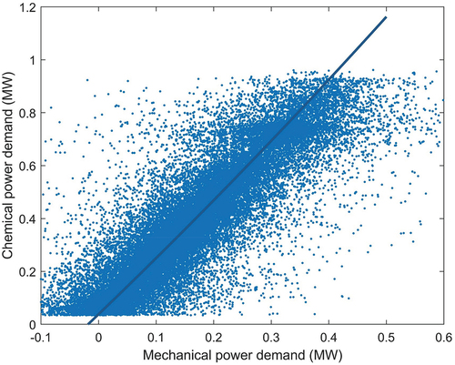
It should be noted that the model includes engine and gear box friction losses, the power to drive auxiliary units etc. For a mechanical power of zero, the model corresponds to a fuel flow of 4 liters per hour, which is slightly higher than observed idle fuel consumption for heavy trucks, but consistent with the fact that average engine speed and thus friction and pumping losses are higher than at idle.

Results

Evaluation of the driver model

For the intended purpose, there are two requirements on the driver model. Firstly, it should with sufficient accuracy predict the expected time to complete a route. Secondly, the output should have the quality necessary to predict energy use. Also for an elaborate model, there are limits on the predictability on route level. Ultimately, driving is subject to variability even when the conditions are similar, and this puts a limit on the attainable accuracy for any driver model. A demonstration is given in Figure 7, which shows the speed profile of a truck driving the same 16 km route six times in 9 hours.

Figure 7. Speed profile of repeated driving cycle for a timber vehicle.

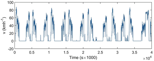
The route is situated in northern Sweden and consists equally of bituminous and (mostly high standard public) gravel road. Good daylight conditions prevail also at night during summertime. The loaded trips took 1146 s, 1145 s, 1250 s, 1140 s, 1178 s and 1196 s. Of these trips, number 1, 2, 4, and 5 are similar with no intermediate stops. The empty return trips took 1198 s, 1078 s, 1305 s, 1754 s, 1143 s, and 1205 s. Trips 1, 2, 5, and 6 are similar. There is a difference of 10% between the shortest and longest time to cover the same route under (as far as known) similar conditions.

The driver model was evaluated by application on a test data set consisting of 10 randomly selected driving sequences of varying length for each project vehicle. Sequences with stops no longer than 30 s were accepted. The test data was taken from mid-January and mid-May to represent winter and summer conditions. Some cases of speeding were detected in the material. To get a fair comparison, the recorded data was truncated to maximum allowed speed. A comparison between real and simulated driving times is presented in Figure 8 and Table 7. The results show on average a slight over estimation of the driving time. The mean absolute error is in the order of 6%. The evaluation represents an average distribution of driving on private/public roads. In particular cases (private roads of varying and unknown conditions, long stretches of high standard road with cruise control active etc.) the variation can be higher as well as lower.

Figure 8. Comparison between real time and simulated time for a set of driving cycles during winter and summer.

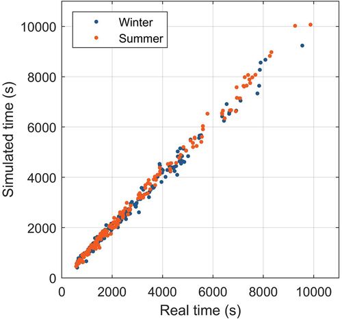
Table 7. Accuracy and precision for the driver simulator during winter and summer.

Accuracy measure	Winter	Summer
Ratio total simulated time/real time	1.010	1.038
RMS error	7.9 %	7.4 %
Avg absolute error	5.6 %	5.8 %

Evaluation of the vehicle response model

The combined driver and vehicle model was evaluated by application on various driving cycles and comparing the result with the measured fuel consumption on the same routes. The same test data set as for the driver response model was used (excepting one vehicle with a faulty engine management system leading to excessive consumption). The same set of average parameters ($C_r$, $C_d$, and drivetrain efficiency) were applied in order to mimic a realistic use case where a general, rather than a specific, vehicle is assumed. Figure 9 and Table 8 present results of the evaluation. As can be seen, the calculations are accurate on average, but there are substantial differences on route level. A justified question is whether the variations are due to the driver model or the vehicle model. Applying the vehicle response model on measured driving cycles, the variations are reduced roughly only by one third, indicating that the culprit is mainly in the vehicle model. Firstly, the vehicle model is very simple with limited capacity to resolve short routes with marked engine transients. Secondly, uncertainty in road elevation data is again an important source of error. A general observation when driving in hilly regions is that it is not so much the steepness when driving uphill that matters, but rather the steepness going downhill. Obviously, uphill driving increases fuel consumption, but this tends to be largely compensated downhill. The compensation works if the downslopes are not so steep as to necessitate braking, though. With this in mind, it is not surprising that inaccurate road elevation data gives errors in energy calculations, although the average road grade for the whole route might be correct.

Figure 9. Comparison of observed and computed fuel consumption for a number of routes of varying length during winter and summer.

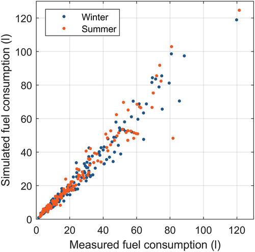
Table 8. Accuracy and precision for the fuel consumption model applied on simulated driving cycles of varying length during winter and summer.

Accuracy measure	Winter	Summer
Ratio simulated/measured fuel volume for trip	0.989	1.01
RMS error	16 %	15 %
Avg absolute error	14 %	11 %

It can be of interest to compare the natural variation also for fuel consumption. The repeated and similar loaded routes of driving cycles 1, 2, 4 and 5 shown in Figure 7 consumed, respectively, 9.70 l, 9.43 l, 9.83 l, and 9.18 l of diesel. The corresponding unloaded routes required 6.88 l, 7.10 l, 6.72 l, and 6.54 l. For this 16 km route, the largest difference between highest and lowest consumption is 9%for the unloaded vehicle and 7% for the loaded vehicle. Loaded weights were 60 tonnes, 51 tonnes, 59 tonnes, and 65 tonnes, respectively. Apparently, the highest and the lowest consumptions do not agree with the weight ranking, so other factors (likely related to the traffic situation) have intervened.

Discussion

Early in the project, questions about representativity were raised by some intended users of the model. Did the data collection represent the whole of Sweden in terms of topography, climatology, and road standard? It is in principle irrelevant whether a hill is situated in the north or in the south. What matters is its physical properties, and by covering a variety of driving conditions a model is developed that minimizes the risk for regionally biased results, which might be the case for models on a more aggregated level. The composition of project vehicles should arguably be randomly selected to represent average conditions. This would however have conflicted with the wish to cover as much as possible of the variation in technical equipment and performance that is seen among timber trucks today. Another factor that makes a randomized study difficult is that participation for practical reasons must be on a voluntary level from the haulers. A consequence of this is that the participators potentially represent a group of haulers that are development oriented and pay a lot of attention to their trucks and their drivers’ competence development. Interviews with the haulers did however not indicate that this is a major problem for the study. The haulers tended to focus somewhat differently on factors such as eco-driving or productivity and the individual drivers have considerable freedom in their work.

The statistical behavior rules describe how different phenomena limit the speed. Arguably, the combined effect of two phenomena can be greater than their individual effects. For instance, one may drive slower on a narrow and curvy road, than on a broad and curvy or a narrow and straight road. The number of potential combinations to consider grows rapidly and in some cases the combined effect might only be apparent. In the case of the narrow, curvy road it may instead be the line of sight that is the limiting factor. It is also reasonable to question if there is a limit on the number of stimuli the human brain can consider simultaneously, in analogy with how one pain stimulus can mask another (Enax-Krumova et al. 2020).

The model may overestimate the speed if there are extraneous variables, such as surface roughness or potholes. An advantage is however that the model can be incrementally expanded as new variables or multicollinearities are identified. In the example with road width and curves, the factors likely interact. Included separately, one factor will dominate. If a limit depending on the combination of curve radius and road width is included, that limit may instead dominate.

Several factors, for which there is no data in the road database, presumably affect speed. A factor that can be expected to be influential especially on unpaved roads is roughness. Although visible only for two of the project’s vehicles, there is a tendency for an unloaded trailer to bounce on rough roads necessitating lower speed than if the trailer is loaded. The two vehicles that showed this behavior statistically were active in a region with poor gravel roads, which suggests that roughness is a real problem.

Vegetation close to the road has a detrimental effect on visibility but can be expected to also keep speed down on straight roads if they are narrow. This is primarily a problem on the lowest standard roads of class 9 without continuous maintenance, but these account for a very small fraction of the total driving distance. Daylight and weather are other factors that can arguably affect driving speed. Technically, it is straightforward to include these factors, but for the purpose of calculating nominal transportation costs, it is more appropriate to use an average since it is not possible to know what at time of day and under what weather conditions a certain transportation will be carried out.

In the recorded driving sequences, there are sometimes stretches of roads where the speed is much lower than can be explained by the road properties. In such cases, it is reasonable to assume that the traffic situation has been limiting or that the driver has intentionally kept a low speed for some reason.

Road texture and roughness affect the rolling resistance, and although related losses can be modeled (Karlsson et al. 2011), necessary information is not available in the road database. There is a correlation between surface condition and road class, and it can be presumed that important roads are smoother than less important roads. An effort was made to identify different rolling resistance values depending on road class, but this did not produce significantly different values.

Lifting axles when driving unloaded is an often-recommended means to save fuel. It is not obvious that this is effective. The definition of rolling resistance presumes a linear relation between wheel load and rolling resistance. The total load, which is unaffected by the number of wheels in contact with ground, determines rolling resistance. However, according to Michelin (2003) $F_{\mathit{rr}}$ is approximately proportional to $N^{0.9}$ for truck tires of super single type. This can be interpreted as a weight dependent rolling resistance coefficient that for a typical timber truck is 14 % higher for the unloaded truck than for the loaded truck. Other studies (Ejsmont et al. 2016) find that the load dependency is small and possibly in the other direction. In that case, should a large effect of lifting axles be observed, it is rather a sign of technical problems such as dragging brakes or misaligned axles. In the present study, no information about lifted trailer axles was available, so a deeper investigation on possible effects could not be pursued.

The assumption that the drivetrain is disengaged during coasting is not fully correct. Final drive, driveshaft and part of the gearbox rotate continuously and offer some resistance. In general, the losses consist of a friction component, proportional to the power, and a viscous component, proportional to rotating speed (Schlegel et al. 2009). The former is negligible during coasting, but the viscous losses can be expected to contribute with a small loss term proportional to vehicle speed. Unfortunately, available data accuracy was not sufficient to also introduce a linear term in $\mathit{v}$ in Equation (5)(5) $\mathit{P}=m_{\mathrm{eff}}\mathit{av}+\mathit{mgv}sin\mathit{\alpha }+C_r\mathit{mgv}+C_d\mathit{A}\frac{\rho v^3}{2}.$(5) and get physically reasonable results. The effect of small linear losses will instead be contained in the other terms, although the dependency on $\mathit{v}$ is not fully correct.

Compared to Svenson and Fjeld (2016) with parameters updated from the project’s data set, the model presented predicts fuel consumption with roughly equivalent mean absolute error, but with RMS error around 8 percent points lower for the test data set. Although the models work differently, outliers in the predictions correlate strongly between the models, again suggesting input data deficiencies as a limiting factor. With respect to driving time, mean absolute and RMS errors of the presented model are, respectively, 7 and 12 percent points lower than for the predictions according to Svenson and Fjeld (2017). The findings suggest that inaccurate road information is currently the main impediment for fuel predictions, whereas for estimation of driving time, focus should be on a sufficiently detailed driver model.

Conclusions

The simulation model presented allows for simulation of driving time with an accuracy comparable to the natural variation in a real traffic situation. The energy model shows a higher level of variation, which could probably be reduced with more accurate road data and a more advanced vehicle model (such as VECTO), at the expense of more difficult use and the need to specify an “average” vehicle.

The project has illuminated the need for accurate road information, of which road grade is the most important for energy predictions. For the driver behavior model, line of sight and surface roughness are the most important factors that are currently not sufficiently covered by the data material.

Apart from time and fuel predictions, the simulation results can potentially be used for a range of tasks such as monitoring of vehicle and road condition. To fully exploit the possibilities, again there is need for road grade information of much higher accuracy than is commonly available.

Acknowledgements

I am indebted to the haulers and drivers who made this study possible through their generous participation in the project.

Disclosure statement

No potential conflict of interest was reported by the author(s).

Additional information

Funding

This research was financed by the Swedish Energy Agency [grant 48154-1].

Notes

1. Biometria is the clearing house for timber and timber transportation contracts in Sweden.

References

- Anttila P, Ojala J, Palander T, Väätäinen K. 2023. The effect of road characteristics on timber truck driving speed and fuel consumption based on visual interpretation of road database and data from fleet management system. Silva Fenn (Hels). 56(4): article id 10798. doi: 10.14214/sf.107984.
- Anttila P, Nummelin T, Väätäinen K, Laitila J, Ala-Ilomäki J, Kilpeläinen A. 2022. Effect of vehicle properties and driving environment on fuel consumption and CO2 emissions of timber trucking based on data from fleet management system. Transp Res Interdisc Persp. 15:100671. doi: 10.1016/j.trip.2022.100671.
- Behrisch M, Bieker L, Erdmann J, Krajzewicz D. 2011. SUMO–simulation of urban mobility: an overview. In Proceedings of SIMUL 2011, The Third International Conference on Advances in System Simulation; October 23–28; Barcelona, Spain. ThinkMind.
- Dayman B. 1976. Tire rolling resistance measurements from coast-down tests. SAE technical paper series 760153. doi: 10.4271/760153.
- Ejsmont J, Taryma S, Ronowski G, Swieczko-Zurek B. 2016. Influence of load and inflation pressure on the tyre rolling resistance. Int J Automot Technol. 17(2):237–244. doi: 10.1007/s12239-016-0023-z.
- Enax-Krumova E, Plaga AC, Schmidt K, Özgül ÖS, Eitner LB, Tegenthoff M, Höffken O. 2020. Painful cutaneous electrical stimulation vs. heat pain as test stimuli in conditioned pain modulation. Brain Sci. 10(10):684. doi: 10.3390/brainsci10100684.
- European Commission. 2018. [accessed 2023 Aug 30]. https://climate.ec.europa.eu/system/files/2018-12/201811_overview_en.pdf.
- European Commission. 2019. Vehicle energy consumption calculation TOOL (VECTO). https://climate.ec.europa.eu/eu-action/transport/road-transport-reducing-co2-emissions-vehicles/vehicle-energy-consumption-calculation-tool-vecto_en.
- Giannelli RA, Nam EK, Helmer K, Younglove T, Scora G, Barth M. 2005. Heavy-duty diesel vehicle fuel consumption modeling based on road load and power train parameters. (No. 2005-01-3549) SAE Technical Paper.
- Griliches Z, Ringstad V. 1970. Error-in-the-variables bias in nonlinear contexts. Econo J Econ Soc. 38(2):368–370. doi: 10.2307/1913020.
- Hammarström U, Karlsson B. 1987. VETO-A computer program for calculation of transport costs as a function of road standard. Technical report. VTI/MEDDELANDE-501. Swedish National Road and Transport Research Institute.
- Hyttinen J. 2022. Truck tyre rolling resistance: experimental testing and constitutive modelling of tyres Doctoral dissertation. KTH Royal Institute of Technology.
- Karlsson R, Hammarström U, Sörensen H, Eriksson O. 2011. Road surface influence on rolling resistance. Coastdown measurements for a car and an HGV. Technical note 24A-2011. Swedish National Road and Transport Research Institute.
- Karlsson M, von Hofsten H, Noreland D, Ekman P, Fattahi S. 2022. Slutrapport för ETTaero2 - Aerodynamisk utformning av tunga timmer- och flisfordon. (Aerodynamic design of heavy roundwood and wood chip vehicles). Skogforsk, arbetsrapport 1120–2022.
- Kerali H. 2004. The HDM-4 road investment model. In: Robinson R, Thagesen B, editors. Road Engineering for Development. 2nd ed. CRC Press; p. 416–438.
- Kharrazi S, Almen M, Frisk E, Nielsen L. 2018. Extending behavioral models to generate mission-based driving cycles for data-driven vehicle development. IEEE Trans Veh Technol. 68(2):1222–1230. doi: 10.1109/TVT.2018.2887031.
- Kitamura R, Kuwahara M, editors 2006. Simulation approaches in transportation analysis: recent advances and challenges.
- Kärhä K, Kortelainen E, Karjalainen A, Haavikko H, Palander T. 2023. Fuel consumption of a high-capacity transport (HCT) vehicle combination for industrial roundwood hauling: a case study of laden timber truck combinations in Finland. Int J For Eng. 34(2):284–293. doi: 10.1080/14942119.2022.2163871.
- Levi MD. 1973. Errors in the variables bias in the presence of correctly measured variables. Econometrica. 41(5):985. doi: 10.2307/1913819.
- Michelin. 2003. The tyre, rolling resistance and fuel savings. Clermont-Ferrand, France: Société de Technologie Michelin. [accessed 2023 Mar 08]. http://docenti.ing.unipi.it/guiggiani-m/Michelin_Tire_Rolling_Resistance.pdf.
- Schlegel C, Hösl A, Diel S. 2009. Detailed loss modelling of vehicle gearboxes. In Proceedings of the 7th International Modelica Conference; Como; Italy; 20–22 September 2009;43:434–443. Linköping University Electronic Press.
- Simwanda M, Sessions J, Boston K, Wing MG. 2015. Modeling biomass transport on single-lane forest roads. For Sci. 61(4):763–773. doi: 10.5849/forsci.14-059.
- Svenson G, Fjeld D. 2016. The impact of road geometry and surface roughness on fuel consumption of logging trucks. Scand J For Res. 31(5):526–536. doi: 10.1080/02827581.2015.1092574.
- Svenson G, Fjeld D. 2017. The impact of road geometry, surface roughness and truck weight on operating speed of logging trucks. Scand J For Res. 32(6):515–527. doi: 10.1080/02827581.2016.1259426.
- Swedish Energy Agency. 2019. Drivmedel 2019 (fuel 2019). Publication ER 2020:26.
- Swedish Road Administration. 2004. Vägar och gators utformning, Linjeföring. (Design of roads and streets. Road alignment). Vägverkets publikation 2004:80. ISSN 1401–9612.
- Swedish Road Administration. 2015. Vägars och gators utformning, Begrepp och grundvärden. (Design of roads and streets. Concepts and default values.). Trafikverkets publikation 2015:090.
- Wang L, Gonder JD, Wood EW, Ragatz AC. 2017. The accuracy and correction of fuel consumption from Controller area network broadcast. No. NREL/CP-5400-67674 Golden, CO (United States): National Renewable Energy Lab. (NREL),
- Watanatada T, Harral C, Paterson W, Dhareshwar A, Bhandari A, Tsunokawa K. 1987. The highway design and maintenance standards model—description of the HDM-III model. Vol. 1, Washington, DC: The World Bank.
- Yang G, Xu H, Wang Z, Tian Z. 2016. Truck acceleration behavior study and acceleration lane length recommendations for metered on-ramps. Int J Transp Sci Technol. 5(2):93–102. doi: 10.1016/j.ijtst.2016.09.006.