Analysis of data from the International Outcome Inventory for Hearing Aids (IOI-HA) using Bayesian Item Response Theory

Abstract

Objective

IOI-HA response data are conventionally analysed assuming that the ordinal responses have interval-scale properties. This study critically considers this assumption and compares the conventional approach with a method using Item Response Theory (IRT).

Design

A Bayesian IRT analysis model was implemented and applied to several IOI-HA data sets.

Study sample

Anonymised IOI-HA responses from 13273 adult users of one or two hearing aids in 11 data sets using the Australian English, Dutch, German and Swedish versions of the IOI-HA.

Results

The raw ordinal responses to IOI-HA items do not represent values on interval scales. Using the conventional rating sum as an overall score introduces a scale error corresponding to about 10 − 15% of the true standard deviation in the population. Some interesting and statistically credible differences were demonstrated among the included data sets.

Conclusions

It is questionable to apply conventional statistical measures like mean, variance, t-tests, etc., on the raw IOI-HA ratings. It is recommended to apply only nonparametric statistical test methods for comparisons of IOI-HA results between groups. The scale error can sometimes cause incorrect conclusions when individual results are compared. The IRT approach is recommended for analysis of individual results.

Keywords:

• Hearing aids
• IOI-HA
• Item Response Theory
• behavioural measures

1. Introduction

The International Outcome Inventory for Hearing Aids (IOI-HA) is a seven-item questionnaire widely used to assess the outcome of hearing rehabilitation. The original English version was designed by Cox et al. (2000) and analysed for its psychometric properties by Cox and Alexander (2002). The questionnaire has (so far) been translated to 30 different languages¹. It is often used clinically for individual follow-up, and it is also used as an outcome measure in quality assurance surveys of client populations.

The seven items address important aspects of the outcome of hearing aid fitting: (1) usage of the hearing aids, (2) benefit, (3) residual activity limitations, (4) overall satisfaction with the hearing aids, (5) residual participation restrictions, (6) impact of hearing problems on others, and (7) impact on general quality of life. Each item has five ordinal response categories, usually displayed such that better outcomes are ordered in the same direction for all questions. As suggested by Cox and Alexander (2002), the responses are conventionally encoded by integer scores ranging from 1 to 5 for each question. The sum or average across the seven items is sometimes used as an overall score (e.g. Hickson, Clutterbuck, and Khan 2010). Factor analysis (FA) of the raw data is commonly used (e.g. Cox and Alexander 2002; Kramer et al. 2002). For comparisons across population studies, the mean response score is usually calculated across subjects in each population for each question and for the overall score. Population differences are sometimes analysed statistically by t-tests or analysis of variance, using the raw response scores as input data. Cox & Alexander (2002) used inter-item correlations, principal component analysis (PCA) and Cronbach's alpha, with the raw ordinal scores as input, to indicate whether the seven items reflect a unidimensional or multidimensional measure. They concluded that a single total score might be adequate for reporting, although the PCA indicated two separate factors. Similar methods have been used in several later evaluations of other language versions of the IOI-HA.

However, statistical analysis measures and methods like the mean, variance, Cronbach's alpha, PCA, FA, etc., are meaningful only if the numerical input values are derived on an interval scale for each item in the questionnaire, that is, the step sizes between response categories must be equal in some well-defined sense (Siegel and Castellan 1988; Bürkner and Vuorre 2019; Liddell and Kruschke 2018). Furthermore, the sum or average across items as a single overall score is meaningful only if the numerical values represent the same scale for all items.

To our knowledge, this fundamental issue has not been discussed in the previous literature about IOI-HA. The raw integer-coded scores have been used uncritically, although it is not at all obvious that the steps between response categories are equal within each item and between items in the questionnaire. The response distributions typically differ markedly between items (Cox and Alexander 2002, Figure 2; Hickson, Clutterbuck, and Khan 2010, Figure 4). This pattern already suggests that it might be questionable to sum the raw ratings across IOI-HA items.

Item Response Theory (IRT) is a family of probabilistic models designed precisely to handle these scaling issues which are common to test instruments for any purpose in social, psychological or educational research. There is a rich literature on IRT, including several text books (e.g. Fox 2010; Nering and Ostini 2010) with good reviews of the literature. Still, IRT has been applied in only a few audiological studies so far (e.g. Mokkink et al. 2010; Demorest, Wark, and Erdman 2011; Chenault et al. 2013; Boeschen-Hospers et al. 2016; Heffernan et al. 2019). Perhaps this is mainly a question of terminology, because the IRT models are actually mathematically very closely related to signal-detection theory and choice models that have a long history of use in psycho-acoustical research (e.g. Thurstone 1927; Bradley and Terry 1952; Luce 1959; Durlach and Braida 1969). The common basic feature of these models is that subjective responses are regarded as indicators (symptoms) that are only probabilistically related to the real individual trait or ability that is to be measured. The true individual trait cannot be directly observed but only indirectly estimated on the basis of test responses. The model treats each response as determined by an outcome of a latent random variable. The location (mean or median) of the probability distribution of that latent variable represents the individual characteristic to be estimated, whereas the response probabilities also depend on other parameters that may differ among test items, even when those items are designed to measure the same trait.

Contrary to conventional IRT methods which determine only a single point estimate for each model parameter, the Bayesian approach (e.g. Fox 2010) treats all model parameters as random variables and estimates a posterior probability distribution for the parameters, based on all observed responses. Thus, the Bayesian result automatically includes a measure of its statistical reliability. Leijon, Henter, and Dahlquist (2016, Section II.A) presents a gentle tutorial on the interpretation of Bayesian analysis results for audiological data.

This study has applied Bayesian IRT to the analysis of 11 data sets obtained in evaluation studies using four different language versions of the IOI-HA. The analysis will answer the following main research questions:

1. Does it matter if we use raw response data or a more sophisticated IRT model for the analysis, that is, does the choice of method have any noticeable consequence for hearing aid benefit evaluations in clinics and in group comparisons?

2. Can we encode ordinal response categories by new numerical values estimated on a single well-defined interval scale, such that the numerical values are equivalent across all IOI-HA items?

3. 3 Are there statistically credible IOI-HA differences between the populations represented by the 11 included evaluation studies?

2. Methods

2.1. Material

Anonymised individual response data were provided by coauthors of this study, obtained from 11 evaluation studies using four different language versions of the IOI-HA: AU-D-05 (Dillon 2006, n ≈ 300), AU-D-10,-19 (Dillon, personal comm., n ≈ 900 + 200, data from 2010, 2019), AU-H-10 (Hickson, Clutterbuck, and Khan 2010, n = 1653), AU-H-10e (Hickson, personal comm., n ≈ 2000), DE-05 (Heuermann, Kinkel, and Tchorz 2005, n = 488, data provided by M. Kinkel), NL-02 (Kramer et al. 2002, n = 505), NL-16 (Kramer, personal comm., n = 314, data from The Netherlands Longitudinal Study on Hearing (NL-SH), around 2016) and SE-17, −18, −19² (Nordqvist 2018, n ≈ 2400 + 2000 + 2500). All these data sets include only adult users of one or two hearing aids. This analysis included only individual records with at most three missing responses among the seven IOI-HA items, so the actual number of records in this study may differ slightly from the original publications. Several other evaluations of the IOI-HA have been published, but only summary response data were available from those studies (Cox and Alexander 2002; Teixeira, da Silva Augusto, and da Silva Caldas Neto 2008; Serbetcioglu et al. 2009; Brännström and Wennerström 2010; Gasparin, Menegotto, and Cunha 2010; Liu et al. 2011; Jespersen, Bille, and Legarth 2014; Paiva et al. 2017; Lopez-Poveda et al. 2017).

2.2. Notation and IRT model

The response data are mathematically denoted as R_si = l meaning that the sth subject gave the lth ordinal response to the ith IOI-HA item. Here, l is an integer index ranging from 1 to L = 5. In the Graded Response³ IRT model, each response is determined by an outcome of a continuous real-valued latent variable Y_si. The lth response is given whenever the latent variable falls within an interval ${\tau }_{i,l-1}<Y_{si}\le ⩽{\tau }_{i,l},$ where the thresholds separating the intervals form an increasing sequence $\left(-\infty ={\tau }_{i,0}<{\tau }_{i,1}<\dots <{\tau }_{i,L}=+\infty \right).$ The thresholds may differ among items but are assumed to be identical for all subjects. The latent variable is drawn from a logistic⁴ probability distribution with location θ_sd and unity⁵ scale. Here, θ_sd is the dth latent trait of the sth subject that determines responses to the item(s) associated with this trait. It is quite possible that only a small number⁶ of traits are sufficient to explain responses to several items, but we cannot know a priori the required number of traits. A principal component analysis (PCA) with varimax rotation (Cox and Alexander 2002) indicated that perhaps only two latent trait dimensions are sufficient to explain the covariance structure of raw ordinal responses to the seven IOI-HA items. For a similar analysis in the Bayesian context, we introduce for each item a one-of-D binary vector $z_i=\left(z_{i1},\dots ,z_{iD}\right)$ with D ≤ I = the number of items, and only one nonzero element z_id=1 indicating that all responses to the ith item are determined by the dth trait.

Using this notation, the conditional probability of any response, given the model parameters, is as follows: (1) $$P\left(R_{si}=l|{\theta }_{sd},{\tau }_i,z_{id}=1\right)=F\left({\tau }_{i,l}-{\theta }_{sd}\right)-F\left({\tau }_{i,l-1}-{\theta }_{sd}\right)$$(1) where F () is the cumulative distribution function for a standard logistic-distributed random variable, (2) $$F\left(x\right) = \frac{1}{1+e^{-x}}$$(2)

This version of the IRT model for IOI-HA responses includes a total of ND subject-specific parameters, with D trait values for each respondent. The model also includes I(L-1) free threshold parameters, with L-1 thresholds for each test item. All these model parameters are estimated from the total data set of all observed responses.

As the subject-specific values θ_sd are defined on the same interval scale for all items, a weighted average $$\overline{{\theta }_s}=\frac{1}{I}{\sum }_{i,d}{z}_{id}{\theta }_{sd}$$ may be used as an overall individual result. This value may be compared to the corresponding raw overall score $$\overline{R_s}=\frac{1}{I}{\sum }_i{R}_{si}$$ that has been conventionally used.

2.3. Hierarchical model for Subpopulations

As this study includes data from several groups of subjects, there may be some systematic differences between the populations from which the subjects were recruited. Therefore, a hierarchical model is designed for the subject- and population-specific parameters, somewhat inspired by the MLIRT model of Fox (2010, Ch. 6). All subjects in the gth group are assumed to have individual trait values drawn from a Gaussian (normal) population distribution with a group-specific mean and a precision (inverse covariance) matrix assumed identical for all groups. These population parameters are also estimated from the observed responses.

The Bayesian approach estimates a posterior probability distribution for all parameters, based on all observed responses. As the complete posterior distribution cannot be expressed in closed form, the posterior density function is represented by a large set of samples which are all equally probable, given the observed data. Further details of this model and the estimation procedure are presented in Appendixes B and C in the Supplementary Material.

The IRT model defines a multivariate predictive distribution of subject-specific traits as defined in Appendix D in the Supplementary Material. To standardise the response scales, the estimated standard deviations for each trait dimension are used to rescale all subject-specific and item-specific parameters, such that the marginal predicted distribution of all rescaled subject traits has unity variance in the global population of which the included subpopulations are representative samples.

3. Results

This section shows results from the IRT model, providing answers to the main research questions. First, the IRT-estimated response-scale properties are presented in Section 3.1. The practical consequences of the nonuniformity of IOI-HA scales are discussed in Section 3.2, answering the first research question. Section 3.3 presents and discusses a standardised set of ordinal response-scale values, as suggested in the second research question. Finally, the differences between the 11 populations represented by the included data sets are presented in Section 3.4.

The IRT model was trained with D = 4 initially allowed trait dimensions, but only three separate trait dimensions were finally effective, one for IOI-HA items (2, 3, 4, 7), one for items (5, 6) and one for the first item. Although this analysis found separate IRT trait dimensions for these three sets of IOI-HA items, the trait variables are still moderately correlated as shown in Table 1.

Table 1. Pearson correlations between the three trait dimensions within each subpopulation, averaged across all included data sets. The three trait dimensions correspond to IOI-HA items Q(2,3,4,7), Q(5, 6) and Q(1).

Trait	Q(5, 6)	Q(1)
Q(2, 3, 4, 7)	0.584	0.585
Q(5, 6)		0.058

3.1. Response scales for IOI-HA items

The frequency distributions of raw ordinal responses to the IOI-HA items are shown in Figure 1, summarised across all subjects in the included data sets. These results are similar to those previously presented by, for example, Cox and Alexander (2002, Figure 2) and Hickson, Clutterbuck, and Khan (2010, Figure 4). The response distributions differ markedly between IOI-HA items. The distributions are also highly skewed, with response 4 or 5 being the most common.

Figure 1. Frequency distributions of raw ordinal responses to the seven IOI-HA items, summed across 13273 subjects in 11 included data sets.

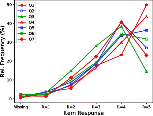
Figure 2. Response intervals as estimated by the IRT model for IOI-HA items. Values on the horizontal axis represent model trait values on the same interval scale for all IOI-HA items, and the plotted response thresholds indicate how trait values are mapped to discrete ordinal responses R = 1,…, 5 for each item. Each plotted response threshold is the model parameter τ_i,l defined in Equation (1)(1) $$P\left(R_{si}=l|{\theta }_{sd},{\tau }_i,z_{id}=1\right)=F\left({\tau }_{i,l}-{\theta }_{sd}\right)-F\left({\tau }_{i,l-1}-{\theta }_{sd}\right)$$(1) , estimated from responses by 13273 subjects in 11 included data sets.

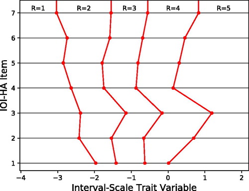
The IRT-estimated response scales, as defined in Equation (1)(1) $$P\left(R_{si}=l|{\theta }_{sd},{\tau }_i,z_{id}=1\right)=F\left({\tau }_{i,l}-{\theta }_{sd}\right)-F\left({\tau }_{i,l-1}-{\theta }_{sd}\right)$$(1) , are shown in Figure 2. The plot shows that the step sizes between ordinal responses are not uniform within each IOI-HA item, and the scales are quite different across items. The resulting probability distributions of ordinal responses are presented in Appendix A in the Supplementary Material.

The differences occur because the distribution of responses is markedly different across items, as noted in earlier studies, and as is evident in Figure 1. For example, relatively few subjects give the highest score on the third IOI-HA question, and few give the lowest score on the seventh item. Therefore, if someone actually gives one of these extreme responses, it is interpreted by the IRT model as a more extreme trait value than for the same ordinal response to other items. Conversely, on the first question, responses of R = 5 (hearing aid use >8 hrs/day) occur in 50% of responses, so do not indicate a very high value (relative to others) on the underlying trait. The zero point on the IRT interval scale corresponds to the response level R = 4 for most items, because this is the median response to those items.

These nonlinearities show that conventional IOI-HA analysis methods are theoretically questionable, because they assume that the raw scores represent a single interval scale. The next section will indicate whether this theoretical issue has any noticeable consequence for hearing aid benefit evaluations in clinics and in group comparisons.

3.2. Raw IOI-HA scores versus IRT traits

The individual raw overall IOI-HA scores and the corresponding individual mean IRT-estimated trait values are plotted in Figure 3(a). The scatter plot indicates a nonlinear relationship between the raw ratings and the IRT-estimated traits. The Spearman rank correlations between the measures are shown in Table 2 for each included subject group. The correlations are, as expected, quite high because both measures are derived from the same data.

Figure 3. Scatter plot of individual overall raw IOI-HA scores (a) and overall re-scaled IOI-HA scores (b) versus the corresponding overall IRT-estimated trait values. A single trait value was calculated for each subject as the mean of the sampled posterior trait distribution. The raw scores have been slightly dithered around their integer values for clarity. The rescaled scores were estimated to place ordinal response values on the same interval scale for all items, as discussed in Section 3.3. Data are included for 13273 subjects in 11 data sets for which individual response data were available.

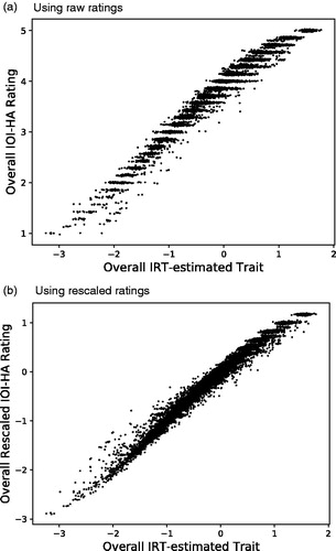
Table 2. Spearman rank correlations between conventional IOI-HA mean ratings and corresponding mean IRT-estimated trait values, for the N subjects in each group.

Group	N	Corr.	Scale error
AU-D-05	311	0.990	15.6%
AU-D-10	912	0.986	11.7%
AU-D-19	203	0.990	12.3%
AU-H-10	1645	0.990	9.6%
AU-H-10e	2061	0.988	9.8%
GE-05	298	0.991	10.5%
NL-02	475	0.987	14.0%
NL-16	314	0.992	8.4%
SE-17	2417	0.987	12.7%
SE-18	2093	0.989	10.7%
SE-19	2544	0.991	11.2%

The “Scale Error” is the conditional standard deviation of individual trait values, normalised by the total trait variance, for any given mean raw score. The scale error has been adjusted to account for the estimation error in individual trait values.

To evaluate the deviation from a perfect correlation, it is interesting to look at the conditional variance of IRT-estimated mean trait values among subjects who showed the same overall mean IOI-HA rating, illustrated by the horizontal spread of the scatter plot at each value on the vertical axis in Figure 3(a). This variance includes two components: 1) A scale error is caused by the nonuniform steps on the IOI-HA rating scales, shown in Figure 2; this causes the mean trait value to differ among subjects even when their mean ratings are identical. 2) An estimation error for individual traits in the IRT model is caused by the Bayesian IRT model calculating a probability distribution of trait values for each subject and each item. When the mean of this posterior distribution is taken as a point estimate of the trait value, the result includes a random uncertainty. However, the variance of this error is easily calculated from the posterior distribution. The final error measure shown in Table 2 has been adjusted to show only the scale error component, after correction for the known trait estimation variance.

The scale nonuniformity can also cause errors when comparing the performance between individuals. Figure 3(a) shows that the IRT-estimated trait difference can sometimes point in the opposite direction to the conventional overall rating difference. Among 83 163 558 pairs of respondents in which one subject had a higher raw score sum than the other, the corresponding IRT-estimated overall traits indicated a difference in the opposite direction in 2% of the pairs. Thus, using only the conventional overall scores may lead to incorrect conclusions in some cases, if the difference is small.

In contrast, the effect of scale nonuniformity is smaller in comparisons between groups of subjects. The scale errors vary with the individual response profile and are therefore partly averaged out. To reveal the effect of scale errors in group comparisons, pairs of subgroups, each with 50 subjects, were drawn at random from the included data sets. Among 19686 pairs where the mean IRT trait difference was greater than 0.05 between the two groups, the group-mean raw overall score and the IRT-estimated mean trait pointed in the opposite directions in only about 0.3% of the pairs.

3.3. Standardised scale for IOI-HA responses

Given an ordinal IOI-HA response on the ith item, the conditional distribution of the corresponding trait value is a truncated normal density, restricted to the response interval. The means of these distributions are listed in Table 3. It might be tempting to use these values to encode the ordinal responses numerically, because these numbers were derived from a standardised common interval scale with zero mean and unity variance for each IOI-HA item, as predicted for a global population for which the included subject groups are representative. However, some serious problems remain.

Table 3. Numerical values that might be used for recoding IOI-HA ordinal responses onto a single interval scale for all items.

Item	R = 1	2	3	4	5
Q1	−2.3	−1.6	−1.0	−0.3	0.8
Q2	−2.7	−1.9	−1.0	0.0	1.3
Q3	−2.7	−1.6	−0.6	0.4	1.7
Q4	−2.9	−2.1	−1.2	−0.3	0.9
Q5	−3.1	−2.1	−1.2	−0.2	1.0
Q6	−3.0	−2.0	−1.1	−0.1	1.1
Q7	−3.3	−2.0	−1.0	0.1	1.4

These scale values are calculated as conditional means within each response interval, when subject-specific trait parameters in the IRT model have been standardised with zero mean and unity predictive variance for all items in the global population of which all the included data sets are representative samples.

The values in Table 3 were used in Figure 3(b) showing the rescaled overall IOI-HA scores versus corresponding overall IRT-estimated trait values. As expected, the resulting scatter plot shows a more linear relationship than for the raw integer scores in Figure 3(a). However, since only a single point value was used to encode each response, the resulting overall rescaled scores still have a discrete distribution with only a finite number of possible outcomes, just like the conventional raw overall score. This is most obvious for the highest scores in the plot.

The distribution of rescaled score points is still considerably skewed towards negative values. In Figure 3(b), the overall IRT trait values extend to about +1.8 on the horizontal axis, whereas the rescaled values on the vertical axis are limited below about +1.2. The reason for this pattern is that the most common raw responses are R = 4 and R = 5 for all items. Therefore, representing these responses by single point values, as in the two rightmost columns of Table 3, gives a somewhat misleading result. For example, the true latent variable for a response R = 5 to the first IOI-HA item might have any value between between 0 and +∞ as indicated in Figure 2. Although the conditional mean value of 0.8 is a good point estimate in this interval, much higher values can also quite often cause the same ordinal response.

For these reasons, the single-point scale values in Table 3 might be used only for evaluations of mean IOI-HA differences between groups. However, for this purpose, there is no obvious practical advantage of using the recoded values instead of the conventional raw ratings. Since the re-scaled results as well as the raw ratings have skewed distributions, nonparametric statistical test methods should be used rather than conventional tools like t-tests or ANOVA, which require normal-distributed data. For comparisons of individual IOI-HA results, or for regression analyses of individual IOI-HA data versus other individual background variables, the probabilistic IRT approach is recommended.

3.4. Population differences

Figure 4 shows that there are some statistically credible differences between IRT results in the subpopulations represented by the included data sets. The joint credibility of these differences is shown in Figure 5. The joint credibility is the predictive probability for the combined event that all the population differences marked by the same or a larger symbol size are true. Thus, the joint credibility accounts for the effect of multiple comparisons, so no further correction is needed for multiple hypothesis tests.

Figure 4. Predictive distributions for three IRT-estimated mean trait values corresponding to IOI-HA items in populations represented by the 11 included data sets. The three separate trait dimensions correspond to subsets of IOI-HA items marked as Q(2,3,4,7), Q(5,6), and Q(1) on the horizontal axis. Symbols indicate medians (equal to means) and vertical lines show 90% symmetric credible intervals for the mean in each population. The right-hand vertical axis shows the trait values transformed back to raw ratings on the seventh “Quality of Life (QoL)” IOI-HA item.

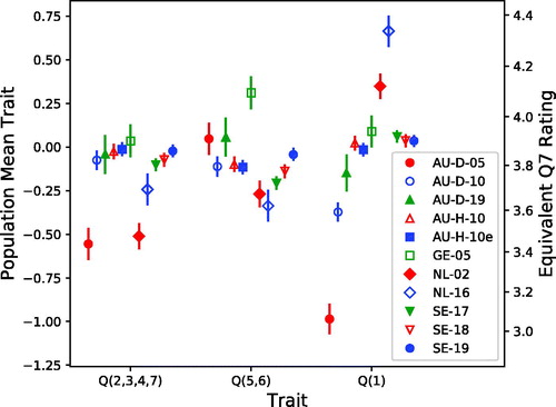
Figure 5. Jointly credible differences between predictive population means for the three IRT-estimated trait values shown in Figure 4. The results for the overall trait mean (d) are calculated with equal weight for the three traits. Each square symbol indicates that the corresponding subpopulation identified on the horizontal axis has a higher mean than the one on the vertical axis. The symbol size indicates the joint credibility of all differences marked by the same or larger symbol. Note that the populations are ordered from greatest to least trait values, independently in each panel.

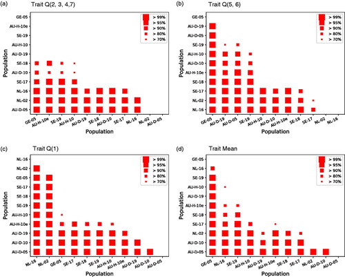
For example, the plot in Figure 5(c) indicates, with a joint credibility greater than 99%, that the mean trait value Q(1) was higher for “NL-16” than for all the other populations, and higher for “NL-02” than for all other up to “GE-05”, and higher for “GE-05” than for all three “AU-D-05, −10, −19”, and for several other comparisons indicated by the same symbol size. The joint credibility is greater than 70%, jointly for all the differences marked in this panel. Similarly, Figure 5(d) indicates that the mean across the three trait dimensions is credibly better in “GE-05” than in all the other populations.

As this analysis included only the IOI-HA data, without any other background variables, it is impossible to determine the reasons for these differences. They are likely caused by a combination of changes across time, differences in hearing loss in the samples and differences in the service system, such as free versus paid, or level of technology employed.

However, the Swedish data sets, “SE-17”, “SE-18” and “SE-19”, were collected in the same way, covering similar populations, so the distribution of other background variables is quite stable over time for these data sets. Results for “SE-19” are clearly better than for “SE-17” and “SE-18” for traits Q(2,3,4,7) and Q(5,6), as well as for the trait mean. The improvement is small but statistically highly credible. This suggests that there may be a trend for increased hearing aid benefit over recent years.

4. Conclusion

A variant of Bayesian Item Response Theory (IRT) has been implemented for the analysis of IOI-HA data and applied to 11 international data sets including a total of 13273 respondents. The analysis method has been implemented as a python package, freely accessible at the Python Package Index⁷. The analysis results support the following conclusions on the research questions:

1. Does it matter if we use raw response data or a more sophisticated IRT model for the analysis?

   Yes. The raw ordinal IOI-HA ratings do not represent values on equivalent interval scales for all items. Using the conventional rating sum as an overall score introduces a scale error corresponding to a measurement error about 10–15% of the true standard deviation for the overall (across-item) trait value in the population. When evaluating the difference between individuals, the conventional overall score and the corresponding IRT-estimated overall trait value sometimes point in different directions. However, the scale error probably has a negligible effect when evaluating the mean difference between groups.

2. Can we encode ordinal response categories by new numerical values that are equivalent across all IOI-HA items?

   Yes, this is possible, but only for evaluating the mean difference between groups, and for this purpose the conventional raw ratings might just as well be used in practice. The recoded data, as well as the raw ratings, have discrete and skewed distributions, so traditional parametric statistical methods like t-test, ANOVA, etc. might give inaccurate results, because these methods assume the input data are normally distributed. It is recommended to apply only nonparametric (rank-based) test methods, if the recoded responses or the conventional raw ratings are used. For analyses of individual IOI-HA results, the probabilistic IRT model is recommended.

3. Are there statistically credible IOI-HA differences between the populations represented by the 11 included data sets?

   Yes, there are some interesting and highly credible differences. Future studies including other background variables, for example age, audiogram and audiological service system, are needed to explain these differences.

Acknowledgements

The authors thank Ben Hornsby for his suggestion to use Item Response Theory as a tool for the analysis of IOI-HA data.

Disclosure statement

No potential conflict of interest was reported by the authors.

Additional information

Funding

This study was approved by the Regional Ethical Review Board, Uppsala, Sweden [2019-03333].

Notes

1 http://icra-audiology.org/Repository/self-report-repository/Survey

2 The complete Swedish Quality Registry for Hearing Rehabilitation included about 30000 individual responses per year from clients using one or two hearing aids. Smaller random subsets from the first half of each year were used here to avoid giving the Swedish data too much weight in the combined result.

3 The Partial Credits Model (Masters, 1982) might be an alternative, but this model was developed primarily for educational assessments where each item is a performance task that requires several steps to reach a complete solution.

4 The Graded Response IRT model can also use the normal distribution.

5 The unity scale is no restriction of generality, as the model scale is arbitrary anyway.

6 Many applications of the IRT model assume all test items to measure a single uni-dimensional individual trait θ_s, so the trait index is omitted. For the IOI-HA application, it seems more appropriate to allow more than one perceptual dimension. A single overall measure is calculated later by averaging across traits.

7 https://pypi.org/project/ItemResponseCalc/

References

- Boeschen-Hospers, J. M., N. Smits, C. Smits, M. Stam, C. B. Terwee, and S. E. Kramer. 2016. “Reevaluation of the Amsterdam Inventory for Auditory Disability and Handicap Using Item Response Theory.” Journal of Speech, Language, and Hearing Research: JSLHR 59 (2): 373–383. doi:10.1044/2015_JSLHR-H-15-0156.
- Bradley, R. A., and M. E. Terry. 1952. “Rank Analysis of Incomplete Block Designs. I. The Method of Paired Comparisons.” Biometrika 39 (3/4): 324–345. doi:10.2307/2334029.
- Brännström, K. J., and I. Wennerström. 2010. “Hearing Aid Fitting Outcome: Clinical Application and Psychometric Properties of a Swedish Translation of the International Outcome Inventory for Hearing Aids (IOI-HA).” Journal of the American Academy of Audiology 21 (8): 512–521. doi:10.3766/jaaa.21.8.3.
- Bürkner, P.-C., and M. Vuorre. 2019. “Ordinal Regression Models in Psychology: A Tutorial.” Advances in Methods and Practices in Psychological Science 2 (1): 77–101. doi:10.1177/2515245918823199.
- Chenault, M., M. Berger, B. Kremer, and L. Anteunis. 2013. “Quantification of Experienced Hearing Problems with Item Response Theory.” American Journal of Audiology 22 (2): 252–262. doi:10.1044/1059-0889(2013/12-0038).
- Cox, R., H. Hyde, S. Gatehouse, W. Noble, H. Dillon, R. Bentler, D. Stephens, et al. 2000. “Optimal Outcome Measures, Research Priorities, and International Cooperation.” Ear and Hearing 21 (4 Suppl): 106S–115S. doi:10.1097/00003446-200008001-00014.
- Cox, R. M., and G. C. Alexander. 2002. “The International Outcome Inventory for Hearing Aids (IOI-HA): Psychometric Properties of the English Version.” International Journal of Audiology 41 (1): 30–35. doi:10.3109/14992020209101309.
- Demorest, M. E., D. J. Wark, and S. A. Erdman. 2011. “Development of the Screening Test for Hearing Problems.” American Journal of Audiology 20 (2): 100–110. doi:10.1044/1059-0889(2011/10-0048).
- Dillon, H. 2006. “Hearing Loss: The Silent Epidemic. Who, Why, Impact and What Can we Do about It. Libby Harricks Oration.” In Self-Help for the Hard of Hearing, Perth, Australia. 17th National Conference of the Audiological Society of Australia.
- Durlach, N., and L. Braida. 1969. “Intensity Perception. I. Preliminary Theory of Intensity Resolution.” The Journal of the Acoustical Society of America 46 (2): 372–383. doi:10.1121/1.1911699.
- Fox, J.-P. 2010. “Bayesian Item Response Modeling: Theory and Applications."New York, NY: Springer.doi: 10.1007/978-1-4419-0742-4
- Gasparin, M., I. H. Menegotto, and C. S. Cunha. 2010. “Psychometric Properties of the International Outcome Inventory for Hearing Aids.” Brazilian Journal of Otorhinolaryngology 76 (1): 85–90. doi:10.1590/S1808-86942010000100014
- Heffernan, E., D. W. Maidment, J. G. Barry, and M. A. Ferguson. 2019. “Refinement and Validation of the Social Participation Restrictions Questionnaire: An Application of Rasch Analysis and Traditional Psychometric Analysis Techniques.” Ear and Hearing 40 (2): 328–339. doi:10.1097/AUD.0000000000000618.
- Heuermann, H., M. Kinkel, and J. R. Tchorz. 2005. “Comparison of Psychometric Properties of the International Outcome Inventory for Hearing Aids (IOI-HA) in Various Studies.” International Journal of Audiology 44 (2): 102–109. doi:10.1080/14992020500031223.
- Hickson, L., S. Clutterbuck, and A. Khan. 2010. “Factors Associated with Hearing Aid Fitting Outcomes on the IOI-HA.” International Journal of Audiology 49 (8): 586–595. doi:10.3109/14992021003777259.
- Jespersen, C. T., M. Bille, and J. V. Legarth. 2014. “Psychometric Properties of a Revised Danish Translation of the International Outcome Inventory for Hearing Aids (IOI-HA).” International Journal of Audiology 53 (5): 302–308. doi:10.3109/14992027.2013.874049.
- Kramer, S. E., S. T. Goverts, W. A. Dreschler, M. Boymans, and J. M. Festen. 2002. “International Outcome Inventory for Hearing Aids (IOI-HA): Results from The Netherlands.” International Journal of Audiology 41 (1): 36–41. doi:10.3109/14992020209101310.
- Leijon, A., G. E. Henter, and M. Dahlquist. 2016. “Bayesian Analysis of Phoneme Confusion Matrices.” IEEE/ACM Transactions on Audio, Speech, and Language Processing 24 (3): 469–482. doi:10.1109/TASLP.2015.2512039.
- Liddell, T., and J. K. Kruschke. 2018. “Analyzing Ordinal Data with Metric Models: What Could Possibly Go Wrong?” Journal of Experimental Social Psychology 79: 328–348. doi:10.1109/TASLP.2015.2512039.
- Liu, H., H. Zhang, S. Liu, X. Chen, D. Han, and L. Zhang. 2011. “International Outcome Inventory for Hearing Aids (IOI-HA): Results from the Chinese Version.” International Journal of Audiology 50 (10): 673–678. doi:10.3109/14992027.2011.588966.
- Lopez-Poveda, E. A., P. T. Johannesen, P. Pérez-Gonzalez, J. L. Blanco, S. Kalluri, and B. Edwards. 2017. “Predictors of Hearing-Aid Outcomes.” Trends in Hearing 21: 1–28. doi:10.1177/2331216517730526.
- Luce, R. D. 1959. Individual Choice Behavior: A Theoretical Analysis. New York, NY: Wiley.
- Masters, G. N. 1982. “A Rasch Model for Partial Credit Scoring.” Psychometrika 47 (2): 149–174. doi:10.1007/BF02296272.
- Mokkink, L. B., D. L. Knol, R. M. A. van Nispen, and S. E. Kramer. 2010. “Improving the Quality and Applicability of the Dutch Scales of the Communication Profile for the Hearing Impaired Using IRT.” Journal of Speech, Language, and Hearing Research: JSLHR 53 (3): 556–571. doi:10.1044/1092-4388(2010/09-0035).
- Nering, M. L., and R. Ostini. 2010. Handbook of Polytomous Item Response Theory Models. New York, NY: Routledge.
- Nordqvist, P. 2018. “Hearing Aid Fitting and Big Data – What Factors Make a Difference for the End User.” In World Congress of Audiology, Cape Town: International Society of Audiology.
- Paiva, S. M. M., J. F. C. P. M. Simões, A. M. Diogo Paiva, F. J. F. Castro e Sousa, and J.-P. Bébéar. 2017. “Translation of the International Outcome Inventory for Hearing Aids into Portuguese from Portugal.” BMJ Open 7 (3): e013784. doi:10.1136/bmjopen-2016-013784.
- Serbetcioglu, B., B. Mutlu, G. Kirkim, and S. Uzunoglu. 2009. “Results of Factorial Validity and Reliability of the International Outcome Inventory for Hearing Aids in Turkish.” International Advances in Otology 5 (1): 80–86.
- Siegel, S., and N. J. J. Castellan. 1988. Nonparametric Statistics for the Behavioral Sciences. New York: McGraw-Hill.
- Teixeira, C. F., L. G. da Silva Augusto, and S. da Silva Caldas Neto. 2008. “Prótese Auditiva: satisfação Do Usuário Com Sua Prótese e Com Seu Meio Ambiente (Hearing Aid: user Satisfaction with Their Hearing Aid and with Their Environment).” Revista CEFAC 10 (2): 245–253. doi:10.1590/S1516-18462008000200015.
- Thurstone, L. L. 1927. “A Law of Comparative Judgment.” Psychological Review 34 (4): 273–286. doi:10.1037/h0070288.