Study on switching from position to stiffness control for musculoskeletal-inspired robot arm based on direct sum decomposition

Abstract

This paper presents a method of switching from position to stiffness control for a two-degree-of-freedom robot arm driven by three pairs of antagonistic actuators by applying the position and stiffness controller with the aim of developing a robot arm that can perform tasks involving a change from free to constrained motion. The control law consists of a feedback position controller and a feedforward stiffness controller in joint space. The position controller is a traditional PD feedback. The stiffness controller is designed using a newly developed method for solving the robot redundancy and adjusts joint stiffness through the coactivation of all the actuators. The solution to the redundancy expresses the actuator force space by a direct sum of its three subspaces and gives two independent relationships between actuator forces to joint torques and to joint stiffness. The position and stiffness controller is expected to control the position and the stiffness simultaneously and seamlessly perform tasks that involve changing from free to constrained motion. However, it has been revealed that the PD feedback controller affects the joint stiffness and that the stiffness controller reduces energy efficiency during position control. Therefore, this paper attempts to solve the problem by controlling the free motion with the position controller and by controlling the stiffness after the robot reaches the desired posture with the stiffness controller. Simulation results demonstrate that the proposed method can bring the robot to the desired posture, switch the control smoothly, and generate the desired stiffness.

Keywords:

• Musculoskeletal-inspired robot
• biarticular actuator
• stiffness control
• position control
• direct sum decomposition

1. Introduction

Many researchers have investigated the role of biarticular and antagonist muscles in human libs using musculoskeletal models. Hogan [1] studied the variable stiffness property of a single-joint arm model driven by two opposing spring-like muscles and found that the joint torque and the joint stiffness can be controlled separately by the co-activation of the antagonistic muscles. Hogan [2] analysed the stiffness matrix of the endpoint of a musculoskeletal arm model having biarticular and antagonist muscles and showed that these muscles provide the ability to adjust all components of the stiffness matrix. Robots intended to have the variable stiffness property have been developed by mimicking the human joint drive mechanism [3, 4] since it is accepted that stiffness adjustment is essential for robots to perform tasks involving contact with an environment.

Musculoskeletal-inspired robots are redundant systems since they have more actuators than joints. Thus they have an infinite number of combinations of actuator forces that produce the same joint torques; different combinations result in different stiffness. Therefore, controllers for musculoskeletal-inspired robots require a procedure to select just a single combination of actuator forces producing desired joint torques and stiffness. Such a problem is called the force distribution problem.

Optimization techniques can find a solution that minimizes an objective function and are employed in many studies [5, 6]. Optimization algorithms, however, include numerical evaluations and iterative computations and thus cannot provide an equation relating the joint torques and stiffness to the actuator forces, complicating theoretical controller design and stability analysis.

The pseudo-inverse of the transformation matrix from actuator forces to joint torques can successfully solve the distribution problem. While the pseudo-inverse provides the linear mapping from joint toques to actuator forces, it still requires optimization to determine the actuator forces generating desired stiffness. Tahara [7] used the pseudo-inverse matrix to solve the force distribution problem and controlled the position and damping of their musculoskeletal robot arm. However, they did not refer to a relationship between actuator forces and damping coefficients.

We presented a position and stiffness control law consisting of a PD feedback position controller and a feedforward stiffness controller in joint space based on the direct sum decomposition method for a two-degree-of-freedom robot arm driven by three pairs of antagonistic actuators [8]. The direct sum decomposition method [9] is a newly developed solution to the robot redundancy caused by the six actuators; it expresses the actuator force space by a direct sum of its three subspaces and provides two simple and independent relationships between actuator forces to joint torques and to joint stiffness. Thus the direct sum decomposition allows us to design the position and the stiffness controller separately. The proposed position and stiffness controller are expected to control the position and the stiffness simultaneously and seamlessly perform tasks that involve changing from free to constrained motion. We validated the effectiveness of the proposed position and stiffness controller by individually evaluating the performance of each controller. Simulation results, however, revealed that the PD feedback controller affects the joint stiffness and that the stiffness controller reduces energy efficiency during position control, implying that the use of both PD feedback and stiffness controllers is not appropriate.

In this paper, to develop a robot arm that can perform tasks involving a transition from free motion to constrained motion, we propose a switching method for the position and stiffness controller to solve the above problems. The proposed method controls the free motion using the position controller and the stiffness after the robot reaches the desired posture using the stiffness controller.

This paper is organized as follows. Section 2 presents a mathematical model of a musculoskeletal-inspired robot. Section 3 formulates the distribution problem, presents the direct sum decomposition, and provides a solution to the distribution problem. Section 4 develops a switching method from position to stiffness control in joint space using the position and stiffness controller proposed in [8]. Section 5 carries a numerical simulation and argues about the effectiveness of the proposed controller. The final section concludes this paper.

2. Musculoskeletal-inspired robot arm

2.1. Musculoskeletal-inspired robot arm model

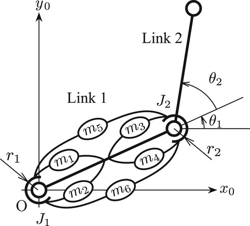
This paper considers a robot arm with two rotational joints, $J_1$ and $J_2$ move in a horizontal plane and mimic the human musculoskeletal system, as shown in Figure 1. The joints are driven by six prismatic actuators $m_1,m_2,\dots ,m_6$. $m_1$ and $m_2$ drive the first joint, $m_3$ and $m_4$ drive the second joint, and $m_5$ and $m_6$ drive both the joints.

Figure 1. Musculoskeletal-inspired robot arm driven by three pairs of antagonistic actuators. $m_1$ and $m_2$ move the first joint, $m_3$ and $m_4$ move the second joint, and $m_5$ and $m_6$ move both joints.

Let ${\theta }_i$ be the angle of joint $J_i$ ($i=1,2$) and $x_j$ be the displacement of actuator $m_j$ ($j=1,2,\dots ,6$). Assuming that the moment arm of each joint is constant regardless of the robot's posture, we have (1) $\mathit{x}=\mathit{Wq},$(1) where $\mathit{q}=[{\theta }_1,{\theta }_2{]}^{\mathrm{T}}$ is the vector of joint angles, and $\mathit{x}=[x_1,x_2,\dots ,x_6{]}^{\mathrm{T}}$ is the vector of actuator displacements. $\mathit{W}$ is a constant matrix describing the routing of the actuators and is given by (2) $\mathit{W}={\left[\begin{array}{cccccc}{r}_1& -r_1& 0& 0& r_1& -r_1\\ 0& 0& r_2& -r_2& r_2& -r_2\end{array}\right]}^{\mathrm{T}},$(2) where $r_i$ is the moment arm of joint $J_i$. Let ${\tau }_i$ be the torque acting on joint $J_i$ ($i=1,2$) and $F_j$ be the output of actuator $m_j$ ($j=1,2,\dots ,6$). Let $\mathit{\tau }$ be the vector of joint torques and $\mathit{F}$ be the vector of actuator outputs, then we have (3) $\mathit{\tau }={\mathit{W}}^{\mathrm{T}}\mathit{F}.$(3)

2.2. Force generation model

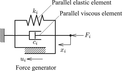
Assume that each actuator consists of a force generator and an elastic and a viscous element parallel to the force generator, as shown in Figure 2. We also assume that the force generator can generate positive and negative forces and that the output $F_i$ of actuator $m_i$ is described by (4) $F_i=u_i-k_i{u}_i{x}_i-c_i{u}_i{\dot{x}}_i,$(4) which is a linear approximation of the Hill model around its natural length [10]. $u_i$ is the force generated by the force generator and is called the active force. Note that the spring constant of the elastic element and the damping coefficient of the viscous element are described by $k_i{u}_i$ and $c_i{u}_i$ and depend on the active force $u_i$.

Figure 2. Force generation model of the actuator. It consists of an elastic element, a viscous element, and a force generator that generates active forces.

Getting together all the output yields (5) $\mathit{F}=\mathit{u}-{\mathit{K}}_x\left(\mathit{u}\right)\mathit{x}-{\mathit{C}}_x\left(\mathit{u}\right)\dot{\mathit{x}}.$(5) ${\mathit{K}}_x\left(\mathit{u}\right)$ and ${\mathit{C}}_x\left(\mathit{u}\right)$ are the stiffness and the viscous matrix with respect to the actuator displacements $\mathit{x}$. They are given by (6) $\begin{array}{rl}{\mathit{K}}_x\left(\mathit{u}\right)& =\mathrm{diag}\left(\begin{array}{cccc}{k}_1{u}_1& k_2{u}_2& \cdots & k_6{u}_6\end{array}\right),\end{array}$(6) (7) $\begin{array}{rl}{\mathit{C}}_x\left(\mathit{u}\right)& =\mathrm{diag}\left(\begin{array}{cccc}{c}_1{u}_1& c_2{u}_2& \cdots & c_6{u}_6\end{array}\right).\end{array}$(7) Combining Equations (1(1) $\mathit{x}=\mathit{Wq},$(1) ), (3(3) $\mathit{\tau }={\mathit{W}}^{\mathrm{T}}\mathit{F}.$(3) ), and (5(5) $\mathit{F}=\mathit{u}-{\mathit{K}}_x\left(\mathit{u}\right)\mathit{x}-{\mathit{C}}_x\left(\mathit{u}\right)\dot{\mathit{x}}.$(5) ), we obtain (8) $\mathit{\tau }={\mathit{W}}^{\mathrm{T}}\mathit{u}-{\mathit{K}}_q\left(\mathit{u}\right)\mathit{q}-{\mathit{C}}_q\left(\mathit{u}\right)\dot{\mathit{q}},$(8) where (9) $\begin{array}{rl}{\mathit{K}}_q\left(\mathit{u}\right)& ={\mathit{W}}^{\mathrm{T}}{\mathit{K}}_x\left(\mathit{u}\right)\mathit{W},\end{array}$(9) (10) $\begin{array}{rl}{\mathit{C}}_q\left(\mathit{u}\right)& ={\mathit{W}}^{\mathrm{T}}{\mathit{C}}_x\left(\mathit{u}\right)\mathit{W},\end{array}$(10) which are called the stiffness and the viscosity matrix in joint space.

2.3. Dynamics

The equations of motion for a standard industrial robot are given by (11) $\mathit{M}\left(\mathit{q}\right)\ddot{\mathit{q}}+\mathit{C}(\mathit{q},\dot{\mathit{q}})\dot{\mathit{q}}=\mathit{\tau }.$(11) $\mathit{M}\left(\mathit{q}\right)$ is the mass matrix, and $\mathit{C}(\mathit{q},\dot{\mathit{q}})\dot{\mathit{q}}$ represents the Coriolis and centrifugal forces. Substituting Equation (8(8) $\mathit{\tau }={\mathit{W}}^{\mathrm{T}}\mathit{u}-{\mathit{K}}_q\left(\mathit{u}\right)\mathit{q}-{\mathit{C}}_q\left(\mathit{u}\right)\dot{\mathit{q}},$(8) ) into Equation (11(11) $\mathit{M}\left(\mathit{q}\right)\ddot{\mathit{q}}+\mathit{C}(\mathit{q},\dot{\mathit{q}})\dot{\mathit{q}}=\mathit{\tau }.$(11) ) leads to the equations of motion of the musculoskeletal-inspired robot arm: (12) $\mathit{M}\left(\mathit{q}\right)\ddot{\mathit{q}}+\mathit{C}(\mathit{q},\dot{\mathit{q}})\dot{\mathit{q}}+{\mathit{C}}_q\left(\mathit{u}\right)\dot{\mathit{q}}+{\mathit{K}}_q\left(\mathit{u}\right)\mathit{q}={\mathit{W}}^{\mathrm{T}}\mathit{u}.$(12) The right-hand side of the above equation represents the joint torques that can be used to control the robot motion. The third term on the left-hand side is the viscous torques due to the parallel viscous element, and the fourth term is the restoring torques due to the parallel elastic element, both of which depend on the active force $\mathit{u}$. Therefore, we can control the motion, viscosity, and stiffness through the coactivation of the active forces.

3. Active force distribution problem

3.1. Active force distribution problem

In this research, we focus on the control of the position and stiffness except for the damping and consider the following problem called the active force distribution problem.

Problem 3.1

For a desired joint torque vector ${\mathit{\tau }}_d$ and a desired joint stiffness matrix ${\mathit{K}}_{\mathrm{qd}}$, find an active force vector $\mathit{u}$ such that (13) $\begin{array}{rl}{\mathit{\tau }}_d& ={\mathit{W}}^{\mathrm{T}}\mathit{u},\end{array}$(13) (14) $\begin{array}{rl}{\mathit{K}}_{\mathrm{qd}}& ={\mathit{K}}_q\left(\mathit{u}\right).\end{array}$(14)

3.2. Direct sum decomposition

To find a solution to the force distribution problem, we first define a representation matrix ${\mathit{K}}_m$ describing a linear transformation from an active force vector to a joint stiffness matrix.

Let ${\mathit{k}}_{\mathrm{qi}}\left(\mathit{u}\right)$ be the ith column vector in the joint stiffness matrix ${\mathit{K}}_q\left(\mathit{u}\right)$. We define a column vector ${\mathit{k}}_q\left(\mathit{u}\right)$ formed by stacking ${\mathit{k}}_{\mathrm{qi}}\left(\mathit{u}\right)$ vertically as (15) ${\mathit{k}}_q\left(\mathit{u}\right)=\left[\begin{array}{c}{\mathit{k}}_{q1}\left(\mathit{u}\right)\\ {\mathit{k}}_{q2}\left(\mathit{u}\right)\end{array}\right].$(15) The above equation can be rewritten as (16) ${\mathit{k}}_q\left(\mathit{u}\right)={\mathit{K}}_m\mathit{u},$(16) where ${\mathit{K}}_m$ is defined as (17) ${\mathit{K}}_m=\left[\begin{array}{c}{\mathit{K}}_{q1}\\ {\mathit{K}}_{q2}\end{array}\right],$(17) where (18) $\begin{array}{rl}{\mathit{K}}_{q1}& =\left[\begin{array}{cccccc}{r}_1^2{k}_1& r_1^2{k}_2& 0& 0& r_1^2{k}_5& r_1^2{k}_6\\ 0& 0& 0& 0& r_1{r}_2{k}_5& r_1{r}_2{k}_6\end{array}\right],\end{array}$(18) (19) $\begin{array}{rl}{\mathit{K}}_{q2}& =\left[\begin{array}{cccccc}0& 0& 0& 0& r_1{r}_2{k}_5& r_1{r}_2{k}_6\\ 0& 0& r_2^2{k}_3& r_2^2{k}_4& r_2^2{k}_5& r_2^2{k}_6\end{array}\right].\end{array}$(19) Then the following proposition [9] holds.

Proposition 3.1

Let U be the set of all active force vectors. Assume that the routing of a musculoskeletal-inspired robot is described by (1(1) $\mathit{x}=\mathit{Wq},$(1) ), the force generation of the actuators is governed by (5(5) $\mathit{F}=\mathit{u}-{\mathit{K}}_x\left(\mathit{u}\right)\mathit{x}-{\mathit{C}}_x\left(\mathit{u}\right)\dot{\mathit{x}}.$(5) ), and the force generators can create positive and negative forces. If $k_1=k_2$, $k_3=k_4$, and $k_5=k_6$, then the active force space U can be expressed by the direct sum of its subspaces as (20) $U=U_1\oplus U_2\oplus U_3,$(20) where $U_1=\mathrm{im}\mathit{W}\cap \ker {\mathit{K}}_m$ is the set of all active force vectors that change only the joint toques, $U_2=\mathrm{im}{\mathit{K}}_m^{\mathrm{T}}\cap \ker {\mathit{W}}^{\mathrm{T}}$ is the set of all active force vectors that change only the joint stiffness, and $U_3=\ker {\mathit{W}}^{\mathrm{T}}\cap \ker {\mathit{K}}_m$ is the set of all active force vectors that changes neither the joint torques nor the joint stiffness. The bases of $U_1$, $U_2$, and $U_3$ are given by $\{{\hat{\mathit{e}}}_1,{\hat{\mathit{e}}}_2\}$, $\{{\hat{\mathit{e}}}_3,{\hat{\mathit{e}}}_4,{\hat{\mathit{e}}}_5\}$, and $\left\{{\hat{\mathit{e}}}_6\right\}$, respectively, where ${\hat{\mathit{e}}}_i$ are given by (21) $\begin{array}{rl}{\hat{\mathit{e}}}_1& ={\left[\begin{array}{cccccc}-1& 1& 0& 0& -1& 1\end{array}\right]}^{\mathrm{T}},\end{array}$(21) (22) $\begin{array}{rl}{\hat{\mathit{e}}}_2& ={\left[\begin{array}{cccccc}0& 0& -1& 1& -1& 1\end{array}\right]}^{\mathrm{T}},\end{array}$(22) (23) $\begin{array}{rl}{\hat{\mathit{e}}}_3& ={\left[\begin{array}{cccccc}1& 1& 0& 0& 0& 0\end{array}\right]}^{\mathrm{T}},\end{array}$(23) (24) $\begin{array}{rl}{\hat{\mathit{e}}}_4& ={\left[\begin{array}{cccccc}0& 0& 1& 1& 0& 0\end{array}\right]}^{\mathrm{T}},\end{array}$(24) (25) $\begin{array}{rl}{\hat{\mathit{e}}}_5& ={\left[\begin{array}{cccccc}0& 0& 0& 0& 1& 1\end{array}\right]}^{\mathrm{T}},\end{array}$(25) (26) $\begin{array}{rl}{\hat{\mathit{e}}}_6& ={\left[\begin{array}{cccccc}-1& 1& -1& 1& 1& -1\end{array}\right]}^{\mathrm{T}}.\end{array}$(26)

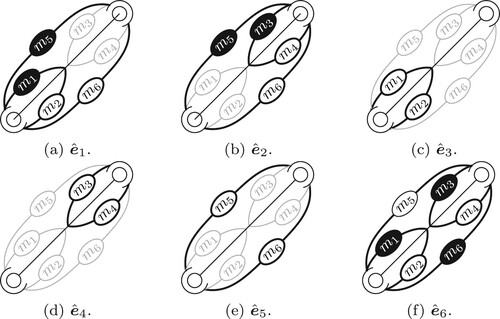
${\hat{\mathit{e}}}_i$ represents a coactivation pattern of actuators $m_i$, as shown in Figure 3. An actuator in white outputs an active force of 1, an actuator in black -1, and an actuator in gray zero. Every active force vector $\mathit{u}$ can be uniquely represented using the new basis as (27) $\mathit{u}={\hat{u}}_1{\hat{\mathit{e}}}_1+{\hat{u}}_2{\hat{\mathit{e}}}_2+\cdots +{\hat{u}}_6{\hat{\mathit{e}}}_6.$(27)

Figure 3. Coactivation pattern of actuators represented by the new bases ${\hat{\mathit{e}}}_1,{\hat{\mathit{e}}}_2,\dots ,{\hat{\mathit{e}}}_6$. The black actuators output a unit active force in the positive direction, the white actuators in the negative direction, and the gray actuators do not output any actives. (a) ${\hat{\mathit{e}}}_1$, (b) ${\hat{\mathit{e}}}_2$, (c) ${\hat{\mathit{e}}}_3$, (d) ${\hat{\mathit{e}}}_4$, (e) ${\hat{\mathit{e}}}_5$, (f) ${\hat{\mathit{e}}}_6$.

3.3. Rewriting active force distribution problem

Applying the above proposition to Equations (13(13) $\begin{array}{rl}{\mathit{\tau }}_d& ={\mathit{W}}^{\mathrm{T}}\mathit{u},\end{array}$(13) ) and (16(16) ${\mathit{k}}_q\left(\mathit{u}\right)={\mathit{K}}_m\mathit{u},$(16) ), we have (28) $\begin{array}{rl}{\mathit{W}}^{\mathrm{T}}\mathit{u}& ={\mathit{W}}^{\mathrm{T}}({\hat{u}}_1{\hat{\mathit{e}}}_1+{\hat{u}}_2{\hat{\mathit{e}}}_2)={\hat{\mathit{W}}}^{\mathrm{T}}{\hat{\mathit{u}}}_{12},\end{array}$(28) (29) $\begin{array}{rl}{\mathit{K}}_m\mathit{u}& ={\mathit{K}}_m({\hat{u}}_3{\hat{\mathit{e}}}_3+{\hat{u}}_4{\hat{\mathit{e}}}_4+{\hat{u}}_5{\hat{\mathit{e}}}_5)={\hat{\mathit{K}}}_m{\hat{\mathit{u}}}_{345},\end{array}$(29) where $\hat{\mathit{W}}$ and ${\hat{\mathit{K}}}_m$ are defined as (30) $\begin{array}{rl}{\hat{\mathit{W}}}^{\mathrm{T}}& ={\mathit{W}}^{\mathrm{T}}\left[\begin{array}{cc}{\hat{\mathit{e}}}_1& {\hat{\mathit{e}}}_2\end{array}\right]\in {\mathbf{R}}^{2\times 2},\end{array}$(30) (31) $\begin{array}{rl}{\hat{\mathit{K}}}_m& ={\mathit{K}}_m\left[\begin{array}{ccc}{\hat{\mathit{e}}}_3& {\hat{\mathit{e}}}_4& {\hat{\mathit{e}}}_5\end{array}\right]\in {\mathbf{R}}^{4\times 3}.\end{array}$(31) ${\hat{\mathit{u}}}_{12}$ and ${\hat{\mathit{u}}}_{345}$ are defined as (32) $\begin{array}{rl}{\hat{\mathit{u}}}_{12}& ={\left[\begin{array}{cc}{\hat{u}}_1& {\hat{u}}_2\end{array}\right]}^{\mathrm{T}},\end{array}$(32) (33) $\begin{array}{rl}{\hat{\mathit{u}}}_{345}& ={\left[\begin{array}{ccc}{\hat{u}}_3& {\hat{u}}_4& {\hat{u}}_5\end{array}\right]}^{\mathrm{T}}.\end{array}$(33) Combining Equations (15(15) ${\mathit{k}}_q\left(\mathit{u}\right)=\left[\begin{array}{c}{\mathit{k}}_{q1}\left(\mathit{u}\right)\\ {\mathit{k}}_{q2}\left(\mathit{u}\right)\end{array}\right].$(15) ), (16(16) ${\mathit{k}}_q\left(\mathit{u}\right)={\mathit{K}}_m\mathit{u},$(16) ), and (29(29) $\begin{array}{rl}{\mathit{K}}_m\mathit{u}& ={\mathit{K}}_m({\hat{u}}_3{\hat{\mathit{e}}}_3+{\hat{u}}_4{\hat{\mathit{e}}}_4+{\hat{u}}_5{\hat{\mathit{e}}}_5)={\hat{\mathit{K}}}_m{\hat{\mathit{u}}}_{345},\end{array}$(29) ), we obtain (34) $\left[\begin{array}{c}{\mathit{k}}_{q1}\left(\mathit{u}\right)\\ {\mathit{k}}_{q2}\left(\mathit{u}\right)\end{array}\right]={\hat{\mathit{K}}}_m{\hat{\mathit{u}}}_{345}\stackrel{\mathrm{△}}{=}\left[\begin{array}{c}{\hat{\mathit{k}}}_{q1}\left({\hat{\mathit{u}}}_{345}\right)\\ {\hat{\mathit{k}}}_{q2}\left({\hat{\mathit{u}}}_{345}\right)\end{array}\right].$(34) Thus the joint stiffness matrix ${\mathit{K}}_q$ can be rewritten as (35) $\begin{array}{rl}{\mathit{K}}_q\left(\mathit{u}\right)& =\left[\begin{array}{cc}{\mathit{k}}_{q1}\left(\mathit{u}\right)& {\mathit{k}}_{q2}\left(\mathit{u}\right)\end{array}\right]\\ & =\left[\begin{array}{cc}{\hat{\mathit{k}}}_{q1}\left({\hat{\mathit{u}}}_{345}\right)& {\hat{\mathit{k}}}_{q2}\left({\hat{\mathit{u}}}_{345}\right)\end{array}\right]\\ & \stackrel{\mathrm{△}}{=}{\hat{\mathit{K}}}_q\left({\hat{\mathit{u}}}_{345}\right)\in {\mathbf{R}}^{2\times 2}.\end{array}$(35) Therefore, we can rewrite the force distribution problem as follows.

Problem 3.2

For a desired joint torque vector ${\mathit{\tau }}_d$ and a desired joint stiffness matrix ${\mathit{K}}_{\mathrm{qd}}$, find ${\hat{\mathit{u}}}_{12}$ and ${\hat{\mathit{u}}}_{345}$ such that (36) $\begin{array}{rl}{\mathit{\tau }}_d& ={\hat{\mathit{W}}}^{\mathrm{T}}{\hat{\mathit{u}}}_{12},\end{array}$(36) (37) $\begin{array}{rl}{\mathit{K}}_{\mathrm{qd}}& ={\hat{\mathit{K}}}_q\left({\hat{\mathit{u}}}_{345}\right).\end{array}$(37)

Equations (36(36) $\begin{array}{rl}{\mathit{\tau }}_d& ={\hat{\mathit{W}}}^{\mathrm{T}}{\hat{\mathit{u}}}_{12},\end{array}$(36) ) and (37(37) $\begin{array}{rl}{\mathit{K}}_{\mathrm{qd}}& ={\hat{\mathit{K}}}_q\left({\hat{\mathit{u}}}_{345}\right).\end{array}$(37) ) are simple algebraic equations, and ${\hat{\mathit{u}}}_{12}$ and ${\hat{\mathit{u}}}_{345}$ can be easily obtained without numerical evaluations and iterative computations. Moreover, Equations (36(36) $\begin{array}{rl}{\mathit{\tau }}_d& ={\hat{\mathit{W}}}^{\mathrm{T}}{\hat{\mathit{u}}}_{12},\end{array}$(36) ) and (37(37) $\begin{array}{rl}{\mathit{K}}_{\mathrm{qd}}& ={\hat{\mathit{K}}}_q\left({\hat{\mathit{u}}}_{345}\right).\end{array}$(37) ) show that ${\hat{\mathit{u}}}_{12}$ and ${\hat{\mathit{u}}}_{345}$ can be determined independently.

3.4. Solution to active force distribution problem

From Equations (36(36) $\begin{array}{rl}{\mathit{\tau }}_d& ={\hat{\mathit{W}}}^{\mathrm{T}}{\hat{\mathit{u}}}_{12},\end{array}$(36) ) and (37(37) $\begin{array}{rl}{\mathit{K}}_{\mathrm{qd}}& ={\hat{\mathit{K}}}_q\left({\hat{\mathit{u}}}_{345}\right).\end{array}$(37) ), ${\hat{\mathit{u}}}_{12}$ and ${\hat{\mathit{u}}}_{345}$ are obtained as (38) $\begin{array}{rl}{\hat{\mathit{u}}}_{12}& =\frac{1}{6r_1{r}_2}\left[\begin{array}{cc}-2r_2& r_1\\ r_2& -2r_1\end{array}\right]\left[\begin{array}{c}{\tau }_{d1}\\ {\tau }_{d2}\end{array}\right],\end{array}$(38) (39) $\begin{array}{rl}{\hat{\mathit{u}}}_{345}& =\frac{1}{2r_1^2{r}_2^2{k}_1{k}_3{k}_5}{\tilde{\mathit{K}}}_q\left[\begin{array}{c}{K}_{\mathrm{qd}11}\\ K_{\mathrm{qd}12}\\ K_{\mathrm{qd}22}\end{array}\right],\end{array}$(39) where (40) ${\tilde{\mathit{K}}}_q=\left[\begin{array}{ccc}{r}_2^2{k}_3{k}_5& -r_1{r}_2{k}_3{k}_5& 0\\ 0& -r_1{r}_2{k}_5{k}_1& r_1^2{k}_1{k}_5\\ 0& r_1{r}_2{k}_1{k}_3& 0\end{array}\right].$(40) The answer to the force distribution problem, i.e. the active forces that generate the desired torques and stiffness, is given by Equation (27(27) $\mathit{u}={\hat{u}}_1{\hat{\mathit{e}}}_1+{\hat{u}}_2{\hat{\mathit{e}}}_2+\cdots +{\hat{u}}_6{\hat{\mathit{e}}}_6.$(27) ). We set ${\hat{u}}_6$ to zero because ${\hat{\mathit{e}}}_6\in U_3$; ${\hat{u}}_6{\hat{\mathit{e}}}_6=0$ holds for all ${\hat{u}}_6$.

3.5. Joint viscosity matrix

Equations (9(9) $\begin{array}{rl}{\mathit{K}}_q\left(\mathit{u}\right)& ={\mathit{W}}^{\mathrm{T}}{\mathit{K}}_x\left(\mathit{u}\right)\mathit{W},\end{array}$(9) ) and (10(10) $\begin{array}{rl}{\mathit{C}}_q\left(\mathit{u}\right)& ={\mathit{W}}^{\mathrm{T}}{\mathit{C}}_x\left(\mathit{u}\right)\mathit{W},\end{array}$(10) ) imply that the joint viscosity matrix ${\mathit{C}}_q\left(\mathit{u}\right)$ equals the joint stiffness matrix ${\mathit{K}}_q\left(\mathit{u}\right)$ if $c_i=k_i$. Therefore, we employ $c_1=c_2$, $c_3=c_4$, and $c_5=c_6$. Then the joint viscosity matrix depends on ${\mathit{u}}_2\in U_2$, but not ${\mathit{u}}_1\in U_1$, leading to (41) ${\mathit{C}}_q\left(\mathit{u}\right)={\hat{\mathit{C}}}_q\left({\hat{\mathit{u}}}_{345}\right).$(41)

3.6. Rewriting equations of motion

Using Equations (28(28) $\begin{array}{rl}{\mathit{W}}^{\mathrm{T}}\mathit{u}& ={\mathit{W}}^{\mathrm{T}}({\hat{u}}_1{\hat{\mathit{e}}}_1+{\hat{u}}_2{\hat{\mathit{e}}}_2)={\hat{\mathit{W}}}^{\mathrm{T}}{\hat{\mathit{u}}}_{12},\end{array}$(28) ), (35(35) $\begin{array}{rl}{\mathit{K}}_q\left(\mathit{u}\right)& =\left[\begin{array}{cc}{\mathit{k}}_{q1}\left(\mathit{u}\right)& {\mathit{k}}_{q2}\left(\mathit{u}\right)\end{array}\right]\\ & =\left[\begin{array}{cc}{\hat{\mathit{k}}}_{q1}\left({\hat{\mathit{u}}}_{345}\right)& {\hat{\mathit{k}}}_{q2}\left({\hat{\mathit{u}}}_{345}\right)\end{array}\right]\\ & \stackrel{\mathrm{△}}{=}{\hat{\mathit{K}}}_q\left({\hat{\mathit{u}}}_{345}\right)\in {\mathbf{R}}^{2\times 2}.\end{array}$(35) ), and (41(41) ${\mathit{C}}_q\left(\mathit{u}\right)={\hat{\mathit{C}}}_q\left({\hat{\mathit{u}}}_{345}\right).$(41) ), the equations of motion of the musculoskeletal-inspired robot can be rewritten as (42) $\begin{array}{rl}& \mathit{M}\left(\mathit{q}\right)\ddot{\mathit{q}}+\mathit{C}(\mathit{q},\dot{\mathit{q}})\dot{\mathit{q}}+{\hat{\mathit{C}}}_q\left({\hat{\mathit{u}}}_{345}\right)\dot{\mathit{q}}+{\hat{\mathit{K}}}_q\left({\hat{\mathit{u}}}_{345}\right)\mathit{q}\\ & ={\hat{\mathit{W}}}^{\mathrm{T}}{\hat{\mathit{u}}}_{12}.\end{array}$(42) The above equation shows that the motion and the stiffness of the robot can be controlled independently, improving the capability of stiffness control of the musculoskeletal-inspired robot arm.

4. Control of joint position and stiffness

4.1. Position and stiffness controller

Consider the following control law of the position and stiffness in joint space of the musculoskeletal-inspired robot arm [8]: (43) ${\hat{\mathit{W}}}^{\mathrm{T}}{\hat{\mathit{u}}}_{12}=-{\mathit{K}}_v\dot{\mathit{q}}-{\mathit{K}}_p\mathit{e}+{\hat{\mathit{K}}}_q\left({\hat{\mathit{u}}}_{345}\right){\mathit{q}}_d,$(43) where ${\mathit{q}}_d$ is a vector of desired angles, $\mathit{e}=\mathit{q}-{\mathit{q}}_d$ is the angle error vector, and ${\mathit{K}}_v$ and ${\mathit{K}}_p$ are positive definite matrices. The first and second terms on the right-hand side of Equation (43(43) ${\hat{\mathit{W}}}^{\mathrm{T}}{\hat{\mathit{u}}}_{12}=-{\mathit{K}}_v\dot{\mathit{q}}-{\mathit{K}}_p\mathit{e}+{\hat{\mathit{K}}}_q\left({\hat{\mathit{u}}}_{345}\right){\mathit{q}}_d,$(43) ) form a PD feedback law for position control. The third term is a feedforward law for stiffness adjustment and implies that the stiffness controller does not require a force sensor; changing the coactivation of the actuators can control the joint stiffness. ${\hat{\mathit{u}}}_{345}$ is determined using Equation (39(39) $\begin{array}{rl}{\hat{\mathit{u}}}_{345}& =\frac{1}{2r_1^2{r}_2^2{k}_1{k}_3{k}_5}{\tilde{\mathit{K}}}_q\left[\begin{array}{c}{K}_{\mathrm{qd}11}\\ K_{\mathrm{qd}12}\\ K_{\mathrm{qd}22}\end{array}\right],\end{array}$(39) ) so that Equation (37(37) $\begin{array}{rl}{\mathit{K}}_{\mathrm{qd}}& ={\hat{\mathit{K}}}_q\left({\hat{\mathit{u}}}_{345}\right).\end{array}$(37) ) holds. ${\hat{\mathit{u}}}_{12}$ is determined by solving Equation (43(43) ${\hat{\mathit{W}}}^{\mathrm{T}}{\hat{\mathit{u}}}_{12}=-{\mathit{K}}_v\dot{\mathit{q}}-{\mathit{K}}_p\mathit{e}+{\hat{\mathit{K}}}_q\left({\hat{\mathit{u}}}_{345}\right){\mathit{q}}_d,$(43) ) under ${\hat{\mathit{K}}}_q\left({\hat{\mathit{u}}}_{345}\right)={\mathit{K}}_{\mathrm{qd}}$. The controller (43(43) ${\hat{\mathit{W}}}^{\mathrm{T}}{\hat{\mathit{u}}}_{12}=-{\mathit{K}}_v\dot{\mathit{q}}-{\mathit{K}}_p\mathit{e}+{\hat{\mathit{K}}}_q\left({\hat{\mathit{u}}}_{345}\right){\mathit{q}}_d,$(43) ) can asymptotically stabilize the equilibrium point $(\mathit{e},\dot{\mathit{q}})=(\mathbf{0},\mathbf{0})$.

4.2. Switch from position control to stiffness control

Equation (43(43) ${\hat{\mathit{W}}}^{\mathrm{T}}{\hat{\mathit{u}}}_{12}=-{\mathit{K}}_v\dot{\mathit{q}}-{\mathit{K}}_p\mathit{e}+{\hat{\mathit{K}}}_q\left({\hat{\mathit{u}}}_{345}\right){\mathit{q}}_d,$(43) ) suggests that the proposed position and stiffness controller is likely able to simultaneously control the position and the stiffness and thus seamlessly perform tasks that involve transitions from free to constrained motion. In reference [8], we demonstrated the effectiveness of the proposed position and stiffness controller by simulation. Simulation results, however, revealed that the PD feedback controller affects the joint stiffness and that the stiffness controller reduces energy efficiency during position control. The results imply that the simultaneous use of the PD feedback and stiffness controllers is inappropriate.

Considering these results, we consider a task that involves a transition from position control to stiffness control and propose a switching method for the position and stiffness controller (43(43) ${\hat{\mathit{W}}}^{\mathrm{T}}{\hat{\mathit{u}}}_{12}=-{\mathit{K}}_v\dot{\mathit{q}}-{\mathit{K}}_p\mathit{e}+{\hat{\mathit{K}}}_q\left({\hat{\mathit{u}}}_{345}\right){\mathit{q}}_d,$(43) ). The switching method uses the position controller but not the stiffness controller during position control and does the opposite during stiffness control.

5. Simulation

This section investigates the effectiveness of the proposed switching method by simulation. Table 1 shows the physical parameters of the musculoskeletal-inspired robot arm. The spring constants per unit active force were $k_1=k_2=5.56\left[1/\mathrm{m}\right]$, $k_3=k_4=12.7\left[1/\mathrm{m}\right]$, and $k_5=k_6=4.85\left[1/\mathrm{m}\right]$, which were determined by referring to [11], and the damping coefficients per unit active force were $c_i=0.4k_i$ ($i=1,2,\dots ,6$). The MATLAB function ode45 was used to solve the differential equations given by Equation (42(42) $\begin{array}{rl}& \mathit{M}\left(\mathit{q}\right)\ddot{\mathit{q}}+\mathit{C}(\mathit{q},\dot{\mathit{q}})\dot{\mathit{q}}+{\hat{\mathit{C}}}_q\left({\hat{\mathit{u}}}_{345}\right)\dot{\mathit{q}}+{\hat{\mathit{K}}}_q\left({\hat{\mathit{u}}}_{345}\right)\mathit{q}\\ & ={\hat{\mathit{W}}}^{\mathrm{T}}{\hat{\mathit{u}}}_{12}.\end{array}$(42) ).

Table 1. Physical parameters of the musculoskeletal-inspired robot arm.

	First link	Second link	Unit
Length	0.31	0.27	$\left[\mathrm{m}\right]$
Mass	1.93	1.32	$\left[\mathrm{kg}\right]$
Center of mass $(x,y)$	$(0.165,0.05)$	$(0.135,0.03)$	$\left[\mathrm{m}\right]$
Inertia moment	0.141	0.120	$[\mathrm{kg}\cdot {\mathrm{m}}^2]$
Moment arm	0.05	0.035	$\left[\mathrm{m}\right]$

We assigned the robot the following task to verify the effectiveness of the proposed switching method. Moreover, we compared the result of the proposed switching method with the result when using the PD feedback and stiffness controllers simultaneously throughout the simulation (i.e.not switching).

1. Move the hand to the desired position using the PD feedback law consisting of the first and second terms of Equation (43(43) ${\hat{\mathit{W}}}^{\mathrm{T}}{\hat{\mathit{u}}}_{12}=-{\mathit{K}}_v\dot{\mathit{q}}-{\mathit{K}}_p\mathit{e}+{\hat{\mathit{K}}}_q\left({\hat{\mathit{u}}}_{345}\right){\mathit{q}}_d,$(43) ) but not the stiffness control law given by the third term.

2. Switch from position to stiffness control at t = 5 seconds, a while after the end-effector has reached the desired position: activate the stiffness controller and deactivate the PD feedback controller.

3. Apply an external force of 1N to the hand at t = 10 seconds. The angle between the external force and the x-axis of the task coordinate system is varied from 0 to 360 degrees in 5-degree increments.

4. Evaluate the stiffness ellipse at time t = 15 seconds, a while after the robot has arrived at rest under the external force.

The stiffness ellipse represents the tip stiffness properties of the robot and is defined by (44) $\frac{1}{2}{\left(\mathrm{\Delta }\mathit{r}\right)}^{\mathrm{T}}{\mathit{K}}_{\mathrm{qd}}\left(\mathrm{\Delta }\mathit{r}\right)=c,$(44) where $\mathrm{\Delta }\mathit{r}$ is the tip displacement from the desired tip position ${\mathit{r}}_d$, and c is a constant. The stiffness ellipse can be made by computing the work using the external force and the tip displacement $\mathrm{\Delta }\mathit{r}$.

The initial and desired joint angles, ${\mathit{q}}_0$ and ${\mathit{q}}_d$, were determined from the corresponding initial and desired tip positions, ${\mathit{r}}_0$ and ${\mathit{r}}_d$: (45) ${\mathit{r}}_0=\left[\begin{array}{c}0\\ 0.2\end{array}\right],{\mathit{r}}_d=\left[\begin{array}{c}0\\ 0.3\end{array}\right]\left[\mathrm{m}\right].$(45) The desired joint stiffness matrix ${\mathit{K}}_{\mathrm{qd}}$ was determined from the corresponding desired tip stiffness matrix ${\mathit{K}}_{\mathrm{rd}}$ using the following equation: (46) ${\mathit{K}}_{\mathrm{qd}}={\mathit{J}}^{\mathrm{T}}{\mathit{K}}_{\mathrm{rd}}\mathit{J},$(46) where $\mathit{J}$ is the Jacobian matrix at the desired joint angle ${\mathit{q}}_d$, and the desired tip stiffness ${\mathit{K}}_{\mathrm{rd}}$ was set as follows: (47) ${\mathit{K}}_{\mathrm{rd}}=\left[\begin{array}{cc}30& -3\\ -3& 30\end{array}\right]\left[\mathrm{N}/\mathrm{m}\right].$(47) The feedback gains were set as follows: (48) $\begin{array}{rl}{\mathit{K}}_p& =\left[\begin{array}{cc}27& 9\\ 9& 18\end{array}\right]\left[\mathrm{N}/\mathrm{rad}\right],\end{array}$(48) (49) $\begin{array}{rl}{\mathit{K}}_v& =0.3{\mathit{K}}_p=\left[\begin{array}{cc}9& 3\\ 3& 6\end{array}\right][\mathrm{N}\cdot \mathrm{s}/\mathrm{rad}].\end{array}$(49) Figure 4 shows the stiffness ellipse. The red crosses indicate the stiffness ellipse using the proposed switching method, the blue dots indicate the stiffness ellipse using the PD feedback and stiffness controllers simultaneously throughout the simulation (i.e.not switching), and the green solid line indicates the theoretical result. The figure shows that the proposed switching method can provide the desired tip stiffness but not the simultaneous controller. Equation (43(43) ${\hat{\mathit{W}}}^{\mathrm{T}}{\hat{\mathit{u}}}_{12}=-{\mathit{K}}_v\dot{\mathit{q}}-{\mathit{K}}_p\mathit{e}+{\hat{\mathit{K}}}_q\left({\hat{\mathit{u}}}_{345}\right){\mathit{q}}_d,$(43) ) implies that the PD feedback controller affects the joint stiffness, and thus, the simultaneous controller fails to generate the desired tip stiffness; however, the proposed switching method can overcome this problem by disabling the PD feedback controller in the stiffness control. The difference between the theoretical and stiffness controller results is due to the change in the robot's posture caused by the external force; The desired joint stiffness matrix ${\mathit{K}}_{\mathrm{qd}}$ calculated by Equation (46(46) ${\mathit{K}}_{\mathrm{qd}}={\mathit{J}}^{\mathrm{T}}{\mathit{K}}_{\mathrm{rd}}\mathit{J},$(46) ) is available at the desired joint angle ${\mathit{q}}_d$ and not at other postures.

Figure 4. Stiffness ellipsoid representing the tip stiffness properties.

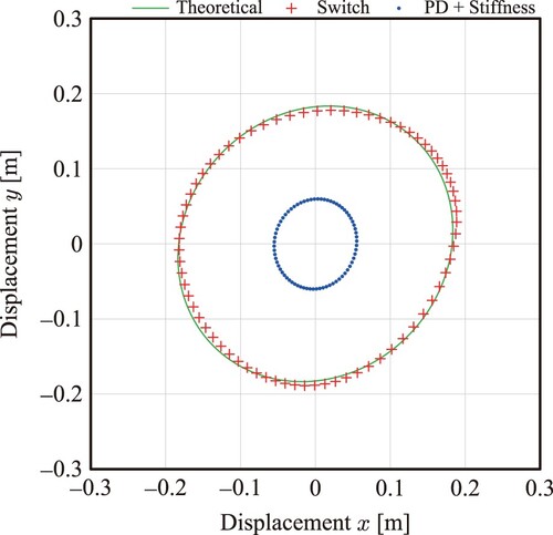
Figure 5 shows the time response of the tip position and velocity when the angle between the external force and the x-axis of the task coordinate system is 45 degrees. The red solid line shows the response using the proposed switching method, the blue dashed line shows the response using the simultaneous PD and stiffness controller, and the green solid line shows the desired value. The figure observes no disturbances in the tip position and velocity around the switching time t = 5 seconds, demonstrating a stable transition from position to stiffness control. Although the responses of the two controllers are almost the same until the end-effector receives the external force, the subsequent behaviours are quite different because of the failure of the stiffness control in the simultaneous control, as mentioned above.

Figure 5. Response of the tip position and velocity. We performed position control in the first five seconds, switched from position control to stiffness control at $t=5$ seconds, and applied an external force to the hand at $t=10$ seconds. (a) Tip position (x-direction), (b) Tip position (y-direction), (c) Tip velocity (x-direction), (d) Tip velocity (y-direction).

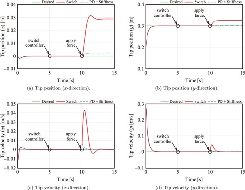
Figure 6 shows the active forces. The red solid line shows the active force using the proposed switching method, and the blue dashed line shows the active force using the simultaneous PD feedback and stiffness controller. Magnified views are provided to clear the small changes in the active forces after the end-effector receives the external force. In the proposed switching method, the active force during position control is given by the sum of the first and second terms of Equation (43(43) ${\hat{\mathit{W}}}^{\mathrm{T}}{\hat{\mathit{u}}}_{12}=-{\mathit{K}}_v\dot{\mathit{q}}-{\mathit{K}}_p\mathit{e}+{\hat{\mathit{K}}}_q\left({\hat{\mathit{u}}}_{345}\right){\mathit{q}}_d,$(43) ), and that during stiffness control is obtained by the third term. In the simultaneous controller, the active force throughout the simulation is given by the sum of all the terms.

Figure 6. Active forces. We performed position control in the first five seconds, switched from position control to stiffness control at t = 5 seconds, and applied an external force to the hand at t = 10 seconds. (a) $m_1$, (b) $m_2$, (c) $m_3$, (d) $m_4$, (e) $m_5$, (f) $m_6$.

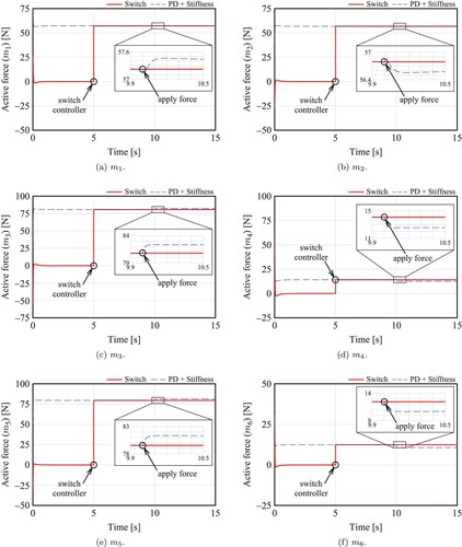
Figure 6 shows that the switching method produces small active forces during position control and large active forces during stiffness control. The large active forces during stiffness control arise from the antagonistic activation of the actuator pairs. Active forces produced by the stiffness controller are expressed by a linear combination of ${\hat{\mathit{e}}}_3$, ${\hat{\mathit{e}}}_4$, and ${\hat{\mathit{e}}}_5\in U_2$, and these basis vectors have activation patterns that antagonistically activate the actuator pairs as shown in Figure 3. The magnified views show that no changes in the active forces of the switching method are observed even though the external force is exerted on the end-effector since the basis vectors have no effect on the joint torques from Theorem 1. Meanwhile, the active forces of the simultaneous controller change slightly when the robot hand is subjected to an external force. This change coincides with the change in the output of the PD feedback controller.

Summarizing the above results, we can conclude that the proposed switching method can achieve the desired stiffness during stiffness control and improve energy efficiency during position control compared to the simultaneous PD feedback and stiffness controller.

6. Conclusion

This paper proposed a method of switching from position to stiffness control of a two-degree-of-freedom musculoskeletal-inspired robot arm utilizing the position and stiffness controller presented in reference [8]. The proposed method switches from position to stiffness control by disabling the position controller and enabling the stiffness controller. The simulation result demonstrated the effectiveness of the proposed switching method; the proposed method can achieve position control with low energy consumption, smooth switching from position to stiffness control, and the desired tip stiffness in stiffness control, resolving the problem arising from the simultaneous use of the position and stiffness controllers. The proposed method could be applied to more complicated tasks involving the transition from free to constrained motion. However, since the proposed controller is designed in joint space, it is unsuitable for controlling position and stiffness in task space, and further improvements are required. Future work will develop the control law in task space and validate its effectiveness using an experiment system.

Disclosure statement

The author reports that there are no competing interests to declare and that no one else except the author has contributed to this study.

Additional information

Funding

No financial support was received for this work.

Notes on contributors

Toshimi Shimizu

Toshimi Shimizu received his Dr. degree from Gifu University in 2003. He joined Niigata University as an assistant in 2004 and Ibaraki University as an associate professor in 2009. His research interests include the control of flexible-link manipulators, musculoskeletal-inspired robot arms.

References

- Hogan N. Adaptive control of mechanical impedance by coactivation of antagonist muscles. IEEE Trans Autom Control. 1984;29(8):681–690. doi: 10.1109/TAC.1984.1103644
- Hogan N. The mechanics of multi-joint posture and movement control. Biol Cybern. 1985;52(5):315–331. doi: 10.1007/BF00355754
- Katayama M, Kawato M. Learning trajectory and force control of an artificial muscle arm by parallel-hierarchical neural network model. Adv Neural Inf Process Syst. 1991;3:436–442.
- Stanev D, Moustakas K. Stiffness modulation of redundant musculoskeletal systems. J Biomech. 2019;85:101–107. doi: 10.1016/j.jbiomech.2019.01.017
- Salvucci V, Kimura Y, Oh S, et al. Force maximization of biarticularly actuated manipulators using infinity norm. IEEE/ASME Trans Mechatron. 2013;18(3):1080–1089. doi: 10.1109/TMECH.2012.2193670
- Jantsch M, Wittmeier S, Dalamagkidis K, et al. Adaptive neural network dynamic surface control: an evaluation on the musculoskeletal robot anthrob. In: Proceedings of 2015 IEEE International Conference on Robotics and Automation; May 2630; Seattle, WA; 2015. doi: 10.1109/ICRA.2015.7139799
- Tahara K, Arimoto S, Sekimoto M, et al. On control of reaching movements for musculo-skeletal redundant arm model. Appl Bionics Biomech. 2009;6(1):11–26. doi: 10.1155/2009/498363
- Toshimi S. Position and stiffness control of musculoskeletal-inspired robot arm based on direct sum decomposition. In: Proceedings of SICE Annual Conference; 2023 Sep 69; Tsu, Japan; 2023.
- Toshimi S. New solution to the force distribution problem for a special class of musculoskeletal robot arms based on direct sum decomposition. Mech Machine Theory. 2020;151:103900. doi: 10.1016/j.mechmachtheory.2020.103900
- Ito K, Tsuji T. Control properties of human-prosthesis systems with bilinear variable structure. In: Mancini G, Martensson L, Johannsen G, editors. Proceedings of 2nd IFAC/IFIP/IFORS/IEA Conference on Analysis, Design and Evaluation of Man-Machine Systems; Sep 10–12; Varese, Italy; 1985. doi: 10.1016/S1474-6670(17)60245-3
- Mera R, Okajima H, Matsunaga N, et al. Stiffness parameter estimation of the muscle for six muscle model using the longitudinal elastic modulus search with gradient method. Jpn J Ergon. 2012;48(4):187–195, (in Japanese).