Testing the suitability of v-Support Vector Machine for hyperspectral image classification

ABSTRACT

This research presents the novel application of v-Support Vector Machine (v-SVM) to hyperspectral image classification. The essence of this work is to test the suitability of v-SVM for hyperspectral image classification. The v-SVM provides an enhancement to the regularisation parameter in the classical Support Vector Machine (SVM). The regularisation parameter controls the trade-off between obtaining a high training error and a low training error which is the ability of the model to generalise the unseen data (or test data). The value of the regularisation parameter in the classical SVM ranges from $0$ to $+\mathrm{\infty }$; this makes it usually challenging to determine the most appropriate optimal regularisation parameter value. The invention of the v-SVM has made it easier to find an appropriate optimal regularisation parameter value since the regularisation parameter is narrowed down from a wide range of $0$ to +$\mathrm{\infty }$ to a narrow range of $0$ to $1$. In this study, two hyperspectral images of Indian Pines region in Northwest Indiana, USA and University of Pavia, Italy are used as test beds for the experiment. The result of the experiment shows that the v-SVM performed fairly better than the classical SVM; however, it fell short of the notable conventional classifiers.

KEYWORDS:

• Remote sensing
• v-Support Vector Machine
• classical support vector machine
• hyperspectral image
• classification

1. Introduction

Hyperspectral Image (HSI) sensors have the capacity of detecting thousands of different bands within the light spectrum (Ding et al. 2023, Yang et al. 2023, Gao et al. 2024, Zhu et al. 2024). HSIs possess high spectral resolution that enables them to detect the spectral properties of objects (Paoletti et al. 2018, Zhao et al. 2019, Shi et al. 2022, Sellami et al. 2023). HSI is an exceedingly robust image that facilitates the exploration of objects’ spectral information with high level of exactitude (Tejasree and Agilandeeswari 2024). They consist of numerous narrow bands that provide a continuous spectral measurement across the entire electromagnetic spectrum (Wang et al. 2019, Okwuashi and Ndehedehe 2020, Cao et al. 2023, Lv et al. 2024). The applications of hyperspectral remote sensing are in numerous areas such as agriculture, ecology, medicine, coastal management, and mineralogy (Imani and Ghassemian 2020, Okwuashi et al. 2022, Dalal et al. 2023, Arshad et al. 2024). Unlike the multispectral image where each pixel has a discrete sample spectrum, each pixel of the HSI has a continuous spectrum, and also the HSI is a more complex image to classifier due to its numerous contiguous spectral bands (Xing et al. 2023, Zhou et al. 2023, Huang et al. 2024).

By the process of image classification, information can be extracted from the HSI (He et al. 2022, Zou et al. 2023). Both classical and modern classifiers have been used for HSI classification. The classical classifiers are models such as K Means (KM), K Nearest Neighbour (KNN), and Gaussian Mixture Model (GMM). While prominent modern classifiers are classifiers such as Artificial Neural Network (ANN) and Support Vector Machine (SVM); nonetheless, our emphasis in this work is on SVM. Zhang et al. (2013) compared the performance of the traditional KM algorithm against the newly developed neighbourhood-constrained k-means (NC-k-means) algorithm for HSI classification. It was found that the new NC-k-means performed better than the traditional KM algorithm. Guo et al. (2018) combined the KNN and guided filter by employing the spectral-spatial technique rather than the traditional pixel-wise technique for HSI classification. The result showed that the spectral-spatial method performed better than the traditional pixel-wise method. Li et al. (2013) applied the GMM for HSI classification after pre-processing, to reduce the dimensionality of data using locality-preserving nonnegative matrix factorisation, as well as local Fisher’s discriminant analysis. The results showed that the proposed technique outperformed traditional approaches.

Several experiments have been done using various types of SVMs. Melgani and Bruzzone (2004) experimented the novel use of SVM for HSI classification. The One Against All (OAA), One Against One (OAO), and two hierarchical tree-based strategies were the four multiclass methods that were experimented. The result of the SVM was compared against those of the ANN and KNN. The results showed that the SVM is an effective alternative to traditional pattern recognition techniques. Archibald and Fann (2007) used the SVM to carryout HSI classification by employing Embedded-Feature-Selection (EFS) algorithm to perform band selection. Guo et al. (2016) employed the SVM to conduct hyperspectral imaging analysis of ripeness evaluation of strawberry. The SVM was used to build classification models on full spectral data, optimal wavelengths, texture features, and the combined dataset of optimal wavelengths and texture features, respectively. Zhang et al. (2022) proposed a method for predicting the mechanical parameters of apples after impact damage based on hyperspectral imaging with the range of 900–1700 nm by non-destructive testing of mechanical parameters using the SVM based on full-band and selected wavelengths. This research introduces the novel use of the v-Support Vector Machine (v-SVM) for HSI classification. The v-SVM was formulated by Schölkopf et al. (2000) and can be applied to both classification and regression problems. Zhao and He (2006) presented an application of the v-SVM to the classification of an unbalanced dataset, whose result showed that the v-SVM outperformed the classical SVM. Zhang and Xie (2007), p. did a forecast of short-term freeway volume with v-SVM. The v-SVM surpassed the classical SVM and the ANN by its ability to overcome local minima and overfitting common with the ANN. We intend to test the suitability of the v-SVM for HSI classification by experimenting it on two HSIs of Indian Pines region in Northwest Indiana, USA, and University of Pavia, Italy. The results will be compared against the traditional SVM and notable conventional classifiers.

2. V-Support Vector Machine

The goal of the SVM is to transform a signal to a higher dimensional feature space and thereafter solve a binary problem in a higher plane (Cortes and Vapnik 1995, Okwuashi and Ndehedehe 2015, Chen et al. 2023). In order to surpass the generalisation capability of the ANN, the SVM is based on structural risk minimisation principle (Wang et al. 2014). Given a dataset $\left(x_i,y_i\right)$, $\mathit{i}=1,2,\dots ,\mathit{N}$; $y_i\mathit{\epsilon }\left\{-1,1\right\}$, $x_i\mathit{\epsilon }{R}^d$, where $x_i$ is the $\mathit{ith}$ data vector that belongs to a binary class $y_i$. The data are separated by the hyperplane $\mathit{f}\left(\mathit{x}\right)=\mathit{w}\cdot \mathit{\varphi }\left(\mathit{x}\right)+\mathit{b}$ provided,

(1) $\left\{\begin{array}{c}\mathit{w}\cdot \mathit{\varphi }\left(\mathit{x}\right)+\mathit{b}\ge +1\mathit{for}{y}_i=+1,\\ \mathit{w}\cdot \mathit{\varphi }\left(\mathit{x}\right)+\mathit{b}\ge -1\mathit{for}{y}_i=-1,\end{array}\right.$(1)

where $\mathit{w}$ is a weight vector and $\mathit{b}$ is a scalar. The separating margin $2/\mathit{w}\cdot \mathit{\varphi }\left(\mathit{x}\right)$ of the classes is a nonlinear function for mapping from a lower dimensional space to a higher dimensional space. Because the samples cannot always be separated by this hyperplane a slack vector $\mathit{\xi }=\left({\xi }_1,{\xi }_2,\cdots ,{\xi }_N\right)$ is introduced to allow the misclassification of some samples. The slack vector is given as,

(2) ${\xi }_i\ge 0,\mathit{\hspace{0.17em}}\mathit{i}=1,2,\cdots ,\mathit{N}.$(2)

By relaxing the constraints the samples can be classified beyond the margins as,

(3) $y_i\left(⟨\mathit{w}\cdot \mathit{\varphi }\left(\mathit{x}\right)⟩+\mathit{b}\right)\ge 1-{\xi }_i\mathit{\hspace{0.17em}},\mathit{i}=1,2,\cdots ,\mathit{N}.\mathit{\hspace{0.17em}}$(3)

Now, for C-SVM, $\mathit{w}$ and $\mathit{\xi }$ is calculated by the minimisation of the objective function,

(4) $\left\{\begin{array}{c}\mathit{\tau }\left(\mathit{w},\mathit{\xi }\right)=\frac{1}{2}\parallel \mathit{w}{\parallel }^2+\mathit{C}\sum _{\mathit{i}=1}^N{\xi }_i\\ \mathit{s}.\mathit{t}.y_i\left(⟨\mathit{w}\cdot \mathit{\varphi }\left(\mathit{x}\right)⟩+\mathit{b}\right)\ge 1-{\xi }_i\mathit{\hspace{0.17em}},\mathit{\hspace{0.17em}}\mathit{i}=1,2,\cdots ,\mathit{N}\end{array}\right.$(4)

where $\mathit{C}$ is the penalty parameter such that $\mathit{C}\ge 0$. We now replace $\mathit{C}$ with another parameter $\mathit{v}$. Therefore equation 4 is rewritten as,

(5) $\left\{\begin{array}{c}\mathit{minimise}\mathit{\tau }\left(\mathit{w},\mathit{\xi },\mathit{\rho }\right)=\frac{1}{2}\parallel \mathit{w}{\parallel }^2-\mathit{v\rho }+\frac{1}{N}\sum _{\mathit{i}=1}^N{\xi }_i\\ \mathit{s}.\mathit{t}.y_i\left(⟨\mathit{w}\cdot \mathit{\varphi }\left(\mathit{x}\right)⟩+\mathit{b}\right)\ge 1-{\xi }_i\mathit{\hspace{0.17em}},\mathit{\hspace{0.17em}}\mathit{i}=1,2,\cdots ,\mathit{N}\mathit{\rho }\ge 0\end{array}\right.$(5)

where $0\le \mathit{v}\le 1$ denotes an upper bound and $2\mathit{\rho }/\parallel \mathit{w}\parallel$ is the separating margin of v-SVM.

The solution of equation 5 can be found by the following dual Lagrange equation,

(6) $\left\{\begin{array}{c}\mathit{maximise}\mathit{\tau }\left(\mathit{\alpha }\right)=-\sum _{\mathit{i},\mathit{j}=1}^N{\alpha }_i{\alpha }_j{y}_i{y}_j\mathit{K}\left(x_i,\mathit{x}\right)\\ \mathit{s}.\mathit{t}.\sum _{\mathit{i}=1}^N{\alpha }_i{y}_i=0;0\le {\alpha }_i\le \frac{1}{N};\sum _{\mathit{i}=1}^N{\alpha }_i\ge \mathit{v}\end{array}\right.$(6)

where $\mathit{K}\left(x_i,x_j\right)=⟨\mathit{\varphi }\left(x_i\right)\cdot \mathit{\varphi }\left(x_j\right)⟩$ is a kernel function, and $\mathit{\alpha }=\left({\alpha }_1,{\alpha }_2,\cdots ,{\alpha }_N\right)$ is called the Lagrange multipliers.

The following equation establishes the relationship between $\mathit{w}$ and $\mathit{\alpha }$,

(7) $\mathit{w}=\sum _{\mathit{i}=1}^N{\alpha }_i{y}_i{x}_i$(7)

The relationship between $\mathit{\rho }$ and b based on the Karush-Kuhn-Tucker (KKT) condition is given as,

(8) $\mathit{\rho }+\mathit{b}=\frac{{\sum }_{0<{\alpha }_i<1/\mathit{N},y_i=+1}\mathrm{\nabla W}\left({\alpha }_i\right)}{{\sum }_{0<{\alpha }_i<1/\mathit{N},y_i=+1}1}$(8)

(9) $\mathit{\rho }-\mathit{b}=\frac{{\sum }_{0<{\alpha }_i<1/\mathit{N},y_i=-1}\mathrm{\nabla W}\left({\alpha }_i\right)}{{\sum }_{0<{\alpha }_i<1/\mathit{N},y_i=-1}1},$(9)

and

(10) $\mathrm{\nabla W}\left({\alpha }_i\right)=\sum _{\mathit{i}=1}^N{\alpha }_i{y}_i{x}_i\mathit{K}\left(x_i,x_j\right).$(10)

We can calculate $\mathit{w}$, $\mathit{\rho }$, and $\mathit{\alpha }$ once $\mathit{v}$ is determined. The corresponding values of $x_i$ where ${\alpha }_i$ values are nonzero called the Support Vectors (SVs). We can determine the class of an input $x_0$ as,

(11) $\mathit{f}\left(x_0\right)=\sum _{\mathit{SVs}}{y}_i{x}_i\mathit{K}\left(x_i,x_j\right)+\mathit{b}$(11)

The binary decision $\left\{+1,-1\right\}$ is $\mathit{f}\left(x_0\right)>0$ for class $+1$, and $\mathit{f}\left(x_0\right)<0$ for class $-1$ (Wang et al. 2014).

3. Implementation

The implementation of the v-SVM was carried out using two HSIs. The first image is a HSI dataset over the Indian Pines region in Northwest Indiana, USA which covers the agricultural fields with regular geometry. Its acquisition was done by the Airborne Visible/Infrared Imaging Spectrometer (AVIRIS). Its pixels scene is 145 × 145with 20 m spatial resolution with 220 spectral bands in the 0.4–2.45$\mathit{\mu }$m region (Figure 1a); and 16 ground-truth classes (Figure 1b). It consists of one-third forest, two-thirds agricultural, and other natural perennial vegetations. The scene was taken in June, hence some of the crops are in the early stages of growth with less than 5% coverage. The second image is a HSI dataset over University of Pavia, Italy acquired by Reflective Optics Spectrographic Image System (ROSIS-03) sensor over the urban area of the University of Pavia, Italy (Figure 1c). It generates 115 spectral bands. It covers the agricultural fields with regular geometry and has a spatial resolution of 1.3 m and a scene that contains 610 × 340 pixels. It consists of 9 ground-truth classes (Figure 1d). The ground-truth enables the comparison of the image data with the real features on the ground and also the gathering of objective dataset for testing the model (Nagai et al. 2020., Okwuashi and Ndehedehe 2021). The ground-truth enhances the discerning, interpretation and analysis of the study area as well as ensuring the proper calibration of remote sensing data (Okwuashi and Ikediashi 2013, Warren and Korotev 2022, Dhiman et al. 2023, Jiang et al. 2024).

Figure 1. (a) False colour image of Indian pines (b) ground truth labels of Indian pines (c) false colour of University of Pavia (d) ground truth labels of University of Pavia.

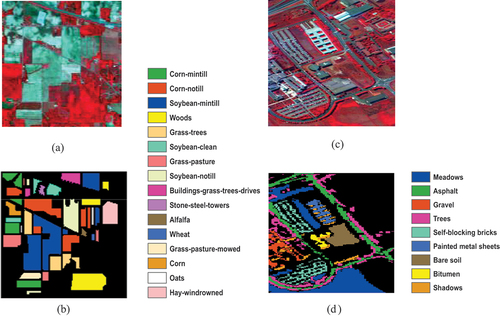
For Indian Pines 1,022 and 9,092 pixels (Table 1) were extracted as training and test datasets respectively; while for University of Pavia 441 and 42,338 pixels (Table 2) were extracted as training and test datasets respectively. The following algorithm gives a brief illustration on how the model was implemented. In order to implement the v-SVM, we began by setting the number of iterations to 1 (that is $\mathit{t}=1$). We input $x_i$ and $y_i$, then using the Gaussian Radial Basis Function kernel (GRBF) kernel $\mathit{K}\left(x_i,\mathit{x}\right)=\mathit{exp}\left(-\parallel x_i-\mathit{x}{\parallel }^2/2{\gamma }^2\right)$ we initialised and determined the values of the kernel parameters and the regularisation parameter, that is for $\mathit{\gamma }\ne 0$ and $0\le \mathit{v}\le 1$. Setting ${\alpha }_i=0$ satisfied the KKT condition indicating that the points that yielded ${\alpha }_i=0$ played no role in the classification. Conversely the points that yielded ${\alpha }_i>0$ played a role in the classification. Therefore, for ${\alpha }_i>0$, $\mathit{w}$ was computed as $\mathit{w}={\sum }_{i=1}^N{\alpha }_i{y}_i{x}_i$. The classification of any unknown point was computed as $\mathit{f}\left(x_0\right)={\sum }_{\mathit{SVs}}{y}_i{x}_i\mathit{K}\left(x_i,\mathit{x}\right)+\mathit{b}$. Convergence was achieved when $\parallel {\propto }_{new}^{i+1}-{\propto }_{new}^i\parallel \le \mathit{\epsilon }$, where $\mathit{\epsilon }$ is a constant.

Table 1. Training and test sets for Indian Pines.

Class	Name	Training set	Test set
1	Corn-mintill	84	754
2	Corn-notill	139	1282
3	Soybean-mintill	247	2211
4	Woods	130	1142
5	Grass-trees	74	657
6	Soybean-clean	57	531
7	Grass-pasture	48	436
8	Soybean-notill	95	873
9	Buildings-grass-trees-drives	42	351
10	Stone-steel-towers	10	87
11	Alfalfa	6	41
12	Wheat	8	44
13	Grass-pasture-mowed	8	26
14	Corn	25	211
15	Oats	7	17
16	Hay-windrowned	42	429
Total		1022	9092

Table 2. Training and test sets for University of Pavia.

Class	Name	Training set	Test set
1	Meadows	190	18449
2	Asphalt	66	6562
3	Gravel	21	2079
4	Trees	32	3031
5	Self-blocking bricks	42	3645
6	Painted metal sheets	15	1332
7	Bare soil	49	4980
8	Bitumen	15	1320
9	Shadows	11	940
Total		441	42338

Algorithm

• I. Set $\mathit{t}=1$, where $\mathit{t}$ denotes number of iterations.

• II. Input $x_i$ and $y_i$, then initialise and determine the values of the kernel parameters and the regularisation parameter, that is for $\mathit{\gamma }\ne 0$ and $0\le \mathit{v}\le 1$.

• III. Compute $\mathit{K}\left(x_i,\mathit{x}\right)$

• IV. Set ${\alpha }_i=0$ to satisfy the KKT condition; and if ${\alpha }_i=0$ go to step 1.

• V. Otherwise if ${\alpha }_i>0$ then compute ${\propto }_{new}^i$ and go to step 6.

• VI. Compute $\mathit{w}={\sum }_{i=1}^N{\alpha }_i{y}_i{x}_i.$

• VII. Compute $\mathit{f}\left(x_0\right)={\sum }_{\mathit{SVs}}{y}_i{x}_i\mathit{K}\left(x_i,\mathit{x}\right)+\mathit{b}$.

• VIII. $\mathit{t}=\mathit{t}+1$; end iteration if algorithm converges, that is if $\parallel {\propto }_{new}^{i+1}-{\propto }_{new}^i\parallel \le \mathit{ϵ}$, otherwise go to step 1.

For example if $\mathit{\gamma }=0.8$ the GRBF kernel $\mathit{K}\left(\mathit{x},\mathit{x}{ }^{\mathrm{\prime }}\right)=\mathit{exp}\left(-x_i-x^2/2{\gamma }^2\right)$ can be computed for $x_i$,

$x_i=\left[\begin{array}{cc}0.3& \begin{array}{cc}0.9& \begin{array}{cc}0.1& 0.5\end{array}\end{array}\\ \begin{array}{c}0.2\\ \begin{array}{c}0.5\\ \begin{array}{c}0.1\\ 0.4\end{array}\end{array}\end{array}& \begin{array}{ccc}\begin{array}{c}0.4\\ 0.3\\ \begin{array}{c}0.6\\ 0.3\end{array}\end{array}& \begin{array}{c}0.3\\ 0.1\\ \begin{array}{c}0.2\\ 0.7\end{array}\end{array}& \begin{array}{c}0.9\\ 0.7\\ \begin{array}{c}0.3\\ 0.8\end{array}\end{array}\end{array}\end{array}\right]=\left|\mathit{A}\right|$, and

$\mathit{K}\left(\mathit{exp}\left(-\parallel \mathit{x}-{\mathit{x}\parallel {\mathit{ }}^{\mathrm{\prime }}}^2/2{\gamma }^2\right)\right)=\mathit{exp}\left(-\frac{{\left(\left[\mathit{A}\right]{\left[\mathit{A}\right]}^{\prime }\right)}^2}{2\times {0.8}^2}\right)=\left[\begin{array}{ccc}0.27& 0.27& \begin{array}{ccc}0.33& 0.43& 0.25\end{array}\\ 0.27& 0.24& \begin{array}{ccc}0.30& 0.42& 0.22\end{array}\\ \begin{array}{c}0.33\\ 0.43\\ 0.25\end{array}& \begin{array}{c}0.30\\ 0.42\\ 0.22\end{array}& \begin{array}{ccc}\begin{array}{c}0.37\\ 0.48\\ 0.28\end{array}& \begin{array}{c}0.48\\ 0.58\\ 0.40\end{array}& \begin{array}{c}0.28\\ 0.40\\ 0.19\end{array}\end{array}\end{array}\right].$

Since the v-SVM outputs binary − 1 and + 1 labels, it was modified to a multi-class classifier by adopting the OAA technique. The OAA is one of the most renowned methods of extending binary classifiers to multi-class problems. The OAA is a method that modifies a binary classifier for multi-class classification by classifying each of the classes of interest against the remaining classes (Okwuashi I 2021, Belghit I 2023, Cavalcanti et al. 2024). Figures 2 and 3 showed, a cross-validation procedure to select an optimal kernel parameter value for gamma $\mathit{\gamma }$ (g) and optimal regularization parameter value for $\mathit{v}$; as g was sampled at 0.2, 0.4, 0.6, 0.8, and 1.0 thresholds. For Indian Pines, from Figure 2 apart from $\mathit{g}\left(0.2\right)$ the optimal $\mathit{v}$ value was 0.4. For University of Pavia, from Figure 3 apart from $\mathit{g}\left(0.2\right)$ the optimal $\mathit{v}$ value was 0.2.

Figure 2. Selection of optimal $\mathit{v}$ value at $\mathit{\gamma }$ thresholds for Indian Pines.

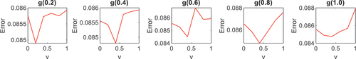
Figure 3. Selection of optimal $\mathit{v}$ value at $\mathit{\gamma }$ thresholds for University of Pavia.

From Figure 4 for Indian Pines, the computed r square values for $\mathit{g}\left(0.2\right)$, $\mathit{g}\left(0.4\right)$, $\mathit{g}\left(0.6\right)$, $\mathit{g}\left(0.8\right)$, $\mathit{g}\left(1.0\right)$ were 0.8926, 0.8992, 0.9626, 0.8718, 0.8370, respectively. While from Figure 5 for University of Pavia, the computed r square values for $\mathit{g}\left(0.2\right)$, $\mathit{g}\left(0.4\right)$, $\mathit{g}\left(0.6\right)$, $\mathit{g}\left(0.8\right)$, and $\mathit{g}\left(1.0\right)$ were 0.8579, 0.8818, 0.9673, 0.8638, and 0.8200, respectively. The results showed that for Indian pines and University of Pavia $\mathit{v}$ was best at 0.2 and 0.4 respectively; while $\mathit{g}$ was best at $\mathit{g}\left(0.6\right)$ for both the Indian pines and University of Pavia.

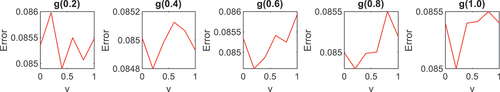
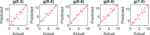
Figure 4. Correlation plots at $\mathit{\gamma }$ thresholds for Indian Pines.

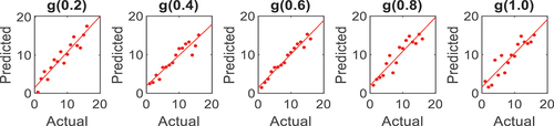
Figure 5. Correlation plots at $\mathit{\gamma }$ thresholds for University of Pavia.

The raw classification results and the overlaid classification results for Indian Pines were shown in Figures 6 and 7 respectively; while the raw classification results and the overlaid classification results for University of Pavia were shown in Figure 8 and 9, respectively. Figure 7 was obtained by overlaying the raw classification results in Figure 6 on the ground-truth data given in Figure 1b; while Figure 9 was obtained by overlaying the raw classification results in Figure 8 on the ground-truth data given in Figure 1d. Tables 3 and 4 contain the classification results for each agricultural class for Indian Pines and University of Pavia, respectively, while the mean classification results of Indian Pines and University of Pavia were displayed in Table 5. The mean classification results for both Indian Pines and University of Pavia indicated that the conventional supervised classifiers (GMM and KNN) performed better than the v-SVM and SVM. The v-SVM performed slightly better than the SVM. The KM is an unsupervised conventional classifier. It can be discerned that the KM yielded a mean classification accuracies of 22.63 and 23.29 for both Indian Pines and University of Pavia, respectively, that are by far lower than the means accuracies of the rest models v-SVM (Indian Pines 76.73 and University of Pavia 76.25), SVM (Indian Pines 73.85 and University of Pavia 73.30), GMM (Indian Pines 88.65 and University of Pavia 89.93), and KNN (Indian Pines 89.67 and University of Pavia 90.98).

Figure 6. Indian Pines raw classification results for v-SVM, SVM, GMM, KNN, and KM.

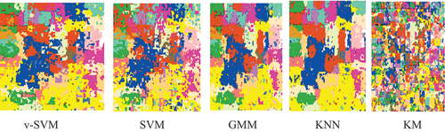
Figure 7. Indian pines overlaid classification results for v-SVM, SVM, GMM, KNN, and KM.

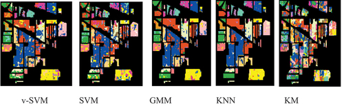
Figure 8. University of Pavia raw classification results for v-SVM, SVM, GMM, KNN, and KM.

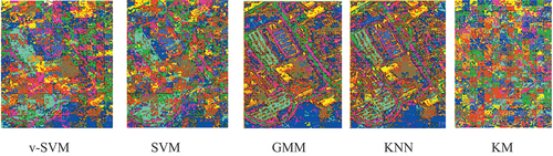
Figure 9. University of Pavia overlaid classification results for v-SVM, SVM, GMM, KNN, and KM.

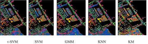
Table 3. Classification accuracy for Indian pines.

		Models
Class	Name	v-SVM	SVM	GMM	KNN	KM
1	Corn-mintill	75.95	74.82	92.68	92.06	22.87
2	Corn-notill	72.02	71.87	87.73	88.50	20.10
3	Soybean-mintill	76.24	73.09	90.42	94.74	28.84
4	Woods	70.65	69.64	91.08	93.18	19.52
5	Grass-trees	74.86	70.13	90.52	92.85	27.06
6	Soybean-clean	75.75	72.74	91.09	93.11	24.69
7	Grass-pasture	80.34	79.86	90.81	93.59	21.74
8	Soybean-notill	81.78	75.97	90.68	89.54	23.35
9	Buildings-grass-trees-drives	78.45	72.43	90.04	90.81	19.01
10	Stone-steel-towers	87.78	84.99	93.01	94.04	25.84
11	Alfalfa	82.03	81.42	88.43	89.75	22.27
12	Wheat	71.87	68.84	84.56	85.00	18.53
13	Grass-pasture-mowed	77.46	74.75	86.85	86.47	21.98
14	Corn	86.46	84.89	91.17	91.22	25.86
15	Oats	60.75	55.32	75.23	75.96	20.75
16	Hay-windrowned	75.21	70.77	84.10	83.90	19.64

Table 4. Classification accuracy for University of Pavia.

		Models
Class	Name	v-SVM	SVM	GMM	KNN	KM
1	Meadows	74.05	71.13	90.97	90.11	23.54
2	Asphalt	80.72	77.89	91.13	92.72	20.60
3	Gravel	74.03	70.28	86.96	87.65	24.53
4	Trees	76.98	72.56	84.73	86.54	22.45
5	Self-blocking bricks	78.99	75.03	93.56	94.83	23.41
6	Painted metal sheets	69.01	67.66	92.84	93.75	24.38
7	Bare soil	72.64	70.88	88.43	89.97	23.06
8	Bitumen	79.75	75.40	90.52	91.69	25.67
9	Shadows	80.11	78.87	90.19	91.53	22.01

Table 5. Summary of classification accuracies for Indian pines and University of Pavia.

Type	v-SVM	SVM	GMM	KNN	KM
Indian Pines	76.73	73.85	88.65	89.67	22.63
University of Pavia	76.25	73.30	89.93	90.98	23.29

4. Summary and conclusion

Even though the SVM was designed specifically for binary classification, it has been adapted for multiclass tasks (Park et al. 2023, Sahu and Pandey 2023, Egashira 2024, Wan et al. 2024). Since the advent of the SVM, it has experienced several improvements, such as Fuzzy Support Vector Machine (FSVM) (Lin and Wang 2002), Deep Support Vector Machine (DSVM) (Chui et al. 2020), Support Tensor Machine (STM) (Chen et al. 2016), Least Squares Support Vector Machine (LS-SVM) (Suykens and Vandewalle 1999) etc. In this work, we presented the novel v-SVM algorithm that utilises the regularisation parameter $\mathit{v}$ to improve the generalisation capability of the SVM (Chang and Lin 2001). Two HSIs Indian Pines and University of Pavia were used for the experiment. The two HSIs used for the experiment consist of sixteen and nine classes, respectively. The GRBF kernel was used to model the v-SVM. For convenience $\mathit{g}\left(0.2\right)$, $\mathit{g}\left(0.4\right)$, $\mathit{g}\left(0.6\right)$, $\mathit{g}\left(0.8\right)$, $\mathit{g}\left(1.0\right)$ gamma $\mathit{\gamma }$ values were used to find the optimal value of $\mathit{v}$. The optimal values of $\mathit{v}$ found for Indian Pines and University of Pavia were 0.4 and 0.2, respectively. Figures 5 and 6 are correlation plots that enable a statistical illustration between the actual and the predicted data; hence, the higher the computed r square, the higher the classification accuracy.

The advantage the v-SVM has over the traditional SVM is that it constraints the regularisation parameter to $0\le \mathit{v}\le 1$ (Liu and Pender 2015). This makes it easier to determine the best optimal regularisation parameter value, unlike the traditional SVM whose regularisation parameter value ranges from $0$ to $+\mathrm{\infty }$; hence, it is often difficult to determine its best optimal regularisation parameter value (Bai et al. 2013), thereby compromising unseen data (test data) generalisation by the model. The v-SVM was compared against the traditional SVM and three conventional classifiers GMM, KNN, and KM. The mean classification results in Table 5 indicated that v-SVM did fairly better than the traditional SVM. In comparison of the v-SVM with the GMM and KNN, it was found that GMM and KNN outperformed the v-SVM. Of the five models used in this experiment, the KM performed the least. It has been widely reported that conventional multiclass models can outperform the traditional binary SVM, the reason being that the SVM is intrinsically designed for binary tasks, unlike the GMM and KNN that are designed for multiclass tasks. For example, KNN is a nonparametric classifier that is distribution-free, that makes it exceedingly robust against highly skewed distribution (Wang et al. 2022, Lahmiri 2023, Hasan et al. 2024). Nonparametric classifiers are often more powerful than parametric classifiers (Chang and Wang 2006, Sheng and Yu 2023, Parr et al. 2024). Even though the SVM is a nonparametric classifier, its binary nature places it at a disadvantage over conventional multiclass classifiers.

Acknowledgments

Christopher E. Ndehedehe is supported by the Australian Research Council Discovery Early Career Researcher Award (DE230101327).

Disclosure statement

No potential conflict of interest was reported by the author(s).

References

- Archibald, R. and Fann, G., 2007. Feature selection and classification of hyperspectral images with support vector machines. IEEE Geoscience and Remote Sensing Letters, 4 (4), 674–677. doi:10.1109/LGRS.2007.905116
- Arshad, T., Zhang, J., and Ullah, I., 2024. A hybrid convolution transformer for hyperspectral image classification. European Journal of Remote Sensing, 2330979. doi:10.1080/22797254.2024.2330979
- Bai, J., Wang, J., and Zhang, X., 2013. A parameters optimization method of v-Support Vector Machineupport vector machine and its application in speech recognition. Journal of Computing, 8 (1), 113–120. doi:10.4304/jcp.8.1.113-120
- Belghit, A., et al. 2023. Optimization of one versus all-SVM using AdaBoost algorithm for rainfall classification and estimation from multispectral MSG data. Advances in Space Research, 71 (1), 946–963. doi:10.1016/j.asr.2022.08.075
- Cao, C., Duan, H., and Gao, X., 2023. Hyperspectral image classification based on three-dimensional adaptive sampling and improved iterative shrinkage-threshold algorithm. Journal of Visual Communication and Image Representation, 90, 103693. doi:10.1016/j.jvcir.2022.103693
- Cavalcanti, G.D., Soares, R.J., and Araújo, E.L., 2024. Subconcept perturbation-based classifier for within-class multimodal data. Neural Computing and Applications, 36 (5), 2479–2491. doi:10.1007/s00521-023-09144-1
- Chang, C.C. and Lin, C.J., 2001. Training v-support vector classifiers: theory and algorithms. Neural Computation, 13 (9), 2119–2147. doi:10.1162/089976601750399335
- Chang, L.Y. and Wang, H.W., 2006. Analysis of traffic injury severity: an application of non-parametric classification tree techniques. Accident Analysis & Prevention, 38 (5), 1019–1027. doi:10.1016/j.aap.2006.04.009
- Chen, H., et al. 2023. Incremental learning for transductive Support Vector Machine. Pattern Recognition, 133, 108982. doi:10.1016/j.patcog.2022.108982
- Chen, Y., Wang, K., and Zhong, P., 2016. One-class support tensor machine. Knowledge-Based Systems, 96, 14–28. doi:10.1016/j.knosys.2016.01.007
- Chui, K.T., et al. 2020. Predicting students’ performance with school and family tutoring using generative adversarial network-based deep Support Vector Machine. IEEE Access, 8, 86745–86752. doi:10.1109/ACCESS.2020.2992869
- Cortes, C. and Vapnik, V., 1995. Support-vector networks. Machine Learning, 20 (3), 273–297. doi:10.1007/BF00994018
- Dalal, A.A., et al. 2023. ETR: enhancing transformation reduction for reducing dimensionality and classification complexity in hyperspectral images. Expert Systems with Applications, 213, 118971. doi:10.1016/j.eswa.2022.118971
- Dhiman, G., Bhattacharya, J., and Roy, S., 2023. Soil textures and nutrients estimation using remote sensing data in north india-punjab region. Procedia computer science, 218, 2041–2048. doi:10.1016/j.procs.2023.01.180
- Ding, Y., et al. 2023. Multi-scale receptive fields: Graph attention neural network for hyperspectral image classification. Expert Systems with Applications, 223, 119858. doi:10.1016/j.eswa.2023.119858
- Egashira, K., 2024. Asymptotic properties of multiclass Support Vector Machine under high dimensional settings. Communications in Statistics - Simulation and Computation, 53 (4), 1991–2005. doi:10.1080/03610918.2022.2066693
- Gao, Q., Wu, T., and Wang, S., 2024. SSC-SFN: spectral-spatial non-local segment federated network for hyperspectral image classification with limited labeled samples. International Journal of Digital Earth, 17 (1), 2300319. doi:10.1080/17538947.2023.2300319
- Guo, C., et al. 2016. Hyperspectral imaging analysis for ripeness evaluation of strawberry with Support Vector Machine. Journal of Food Engineering, 179, 11–18. doi:10.1016/j.jfoodeng.2016.01.002
- Guo, Y., et al. 2018. K-Nearest neighbor combined with guided filter for hyperspectral image classification. Procedia Computer Science, 129, 159–165. doi:10.1016/j.procs.2018.03.066
- Hasan, N., Ahmed, N., and Ali, S.M., 2024. Improving sporadic demand forecasting using a modified k-nearest neighbor framework. Engineering Applications of Artificial Intelligence, 129, 107633. doi:10.1016/j.engappai.2023.107633
- He, Z., et al. 2022. Semi-supervised anchor graph ensemble for large-scale hyperspectral image classification. International Journal of Remote Sensing, 43 (5), 1894–1918. doi:10.1080/01431161.2022.2048916
- Huang, S., et al. 2024. Superpixel-based multi-scale multi-instance learning for hyperspectral image classification. Pattern Recognition, 149, 110257. doi:10.1016/j.patcog.2024.110257
- Imani, M. and Ghassemian, H., 2020. An overview on spectral and spatial information fusion for hyperspectral image classification: Current trends and challenges. Information Fusion, 59, 59–83. doi:10.1016/j.inffus.2020.01.007
- Jiang, C., et al. 2024. A vehicle imaging approach to acquire ground truth data for upscaling to satellite data: a case study for estimating harvesting dates. Remote Sensing of Environment, 300, 113894. doi:10.1016/j.rse.2023.113894
- Lahmiri, S., 2023. Integrating convolutional neural networks, kNN, and Bayesian optimization for efficient diagnosis of Alzheimer’s disease in magnetic resonance images. Biomedical Signal Processing and Control, 80, 104375. doi:10.1016/j.bspc.2022.104375
- Lin, C.F. and Wang, S.D., 2002. Fuzzy Support Vector Machines. IEEE Transactions on Neural Networks, 13 (2), 464–471. doi:10.1109/72.991432
- Li, W., Prasad, S., and Fowler, J.E., 2013. Hyperspectral image classification using Gaussian mixture models and Markov random fields. IEEE Geoscience and Remote Sensing Letters, 11 (1), 153–157. doi:10.1109/LGRS.2013.2250905
- Liu, Y. and Pender, G., 2015. A flood inundation modelling using v-Support Vector Machine regression model. Engineering Applications of Artificial Intelligence, 46, 223–231. doi:10.1016/j.engappai.2015.09.014
- Lv, H., et al. 2024. Multi-dimensional deep dense residual networks and multiple kernel learning for hyperspectral image classification. Infrared Physics & Technology, 138, 105265. doi:10.1016/j.infrared.2024.105265
- Melgani, F. and Bruzzone, L., 2004. Classification of hyperspectral remote sensing images with support vector machines. IEEE Transactions on Geoscience and Remote Sensing, 42 (8), 1778–1790. doi:10.1109/TGRS.2004.831865
- Nagai, S., et al. 2020.Importance of the collection of abundant ground‐truth data for accurate detection of spatial and temporal variability of vegetation by satellite remote sensing. In:K. Dontsova, Z. Balogh-Brunstad, and G. Le Roux, ed. Biogeochemical Cycles: Ecological Drivers and Environmental Impact, 223–244 doi:10.1002/9781119413332.ch11
- Okwuashi, O., et al. 2021. Deep support vector machine for PolSAR image classification. International Journal of Remote Sensing, 42 (17), 6498–6536. doi:10.1080/01431161.2021.1939910
- Okwuashi, O. and Ikediashi, D.I., 2013. GIS-based simulation of land use change. Applied GIS, 10 (1), 1–18.
- Okwuashi, O. and Ndehedehe, C., 2015. Digital terrain model height estimation using support vector machine regression. South African Journal of Science, 111 (9/10), 01–05. doi:10.17159/sajs.2015/20140153
- Okwuashi, O. and Ndehedehe, C.E., 2020. Deep support vector machine for hyperspectral image classification. Pattern Recognition, 103, 107298. doi:10.1016/j.patcog.2020.107298
- Okwuashi, O. and Ndehedehe, C.E., 2021. Integrating machine learning with Markov chain and cellular automata models for modelling urban land use change. Remote Sensing Applications: Society and Environment, 21, 100461. doi:10.1016/j.rsase.2020.100461
- Okwuashi, O., Ndehedehe, C.E., and Olayinka, D.N., 2022. Tensor partial least squares for hyperspectral image classification. Geocarto International, 37 (27), 1–16. doi:10.1080/10106049.2022.2129833
- Paoletti, M.E., et al. 2018. A new deep convolutional neural network for fast hyperspectral image classification. ISPRS Journal of Photogrammetry and Remote Sensing, 145, 120–147. doi:10.1016/j.isprsjprs.2017.11.021
- Park, J., et al. 2023. Efficient differentially private kernel support vector classifier for multi-class classification. Information Sciences, 619, 889–907. doi:10.1016/j.ins.2022.10.075
- Parr, T., Hamrick, J., and Wilson, J.D., 2024. Nonparametric feature impact and importance. Information Sciences, 653, 119563. doi:10.1016/j.ins.2023.119563
- Sahu, S.K. and Pandey, M., 2023. An optimal hybrid multiclass SVM for plant leaf disease detection using spatial fuzzy C-Means model. Expert Systems with Applications, 214, 118989. doi:10.1016/j.eswa.2022.118989
- Schölkopf, B., et al. 2000. New support vector algorithms. Neural Computation, 12 (5), 1207–1245. doi:10.1162/089976600300015565
- Sellami, A., Farah, M., and Dalla Mura, M., 2023. Shcnet: a semi-supervised hypergraph convolutional networks based on relevant feature selection for hyperspectral image classification. Pattern Recognition Letters, 165, 98–106. doi:10.1016/j.patrec.2022.12.004
- Sheng, H. and Yu, G., 2023. TNN: a transfer learning classifier based on weighted nearest neighbors. Journal of Multivariate Analysis, 193, 105126. doi:10.1016/j.jmva.2022.105126
- Shi, C., et al. 2022. Explainable scale distillation for hyperspectral image classification. Pattern Recognition, 122, 108316. doi:10.1016/j.patcog.2021.108316
- Suykens, J.A. and Vandewalle, J., 1999. Least squares support vector machine classifiers. Neural Processing Letters, 9 (3), 293–300. doi:10.1023/A:1018628609742
- Tejasree, G. and Agilandeeswari, L., 2024. An extensive review of hyperspectral image classification and prediction: techniques and challenges. Multimedia Tools and Applications, 1–98. doi:10.1007/s11042-024-18562-9
- Wan, H.P., et al. 2024. SS-MASVM: an advanced technique for assessing failure probability of high-dimensional complex systems using the multi-class adaptive support vector machine. Computer Methods in Applied Mechanics and Engineering, 418, 116568. doi:10.1016/j.cma.2023.116568
- Wang, G.F., et al. 2014. Vibration sensor based tool condition monitoring using ν Support Vector Machine and locality preserving projection. Sensors and Actuators A: Physical, 209, 24–32. doi:10.1016/j.sna.2014.01.004
- Wang, Y., Pan, Z., and Dong, J., 2022. A new two-layer nearest neighbor selection method for kNN classifier. Knowledge-Based Systems, 235, 107604. doi:10.1016/j.knosys.2021.107604
- Wang, A., Wang, Y., and Chen, Y., 2019. Hyperspectral image classification based on convolutional neural network and random forest. Remote Sensing Letters, 10 (11), 1086–1094. doi:10.1080/2150704X.2019.1649736
- Warren, P.H. and Korotev, R.L., 2022. Ground truth constraints and remote sensing of lunar highland crust composition. Meteoritics & Planetary Science, 57 (2), 527–557. doi:10.1111/maps.13780
- Xing, C., et al. 2023. Binary feature learning with local spectral context-aware attention for classification of hyperspectral images. Pattern Recognition, 134, 109123. doi:10.1016/j.patcog.2022.109123
- Yang, J., Du, B., and Zhang, L., 2023. From center to surrounding: an interactive learning framework for hyperspectral image classification. ISPRS Journal of Photogrammetry and Remote Sensing, 197, 145–166. doi:10.1016/j.isprsjprs.2023.01.024
- Zhang, B., et al. 2013. A neighbourhood-constrained k-means approach to classify very high spatial resolution hyperspectral imagery. Remote Sensing Letters, 4 (2), 161–170. doi:10.1080/2150704X.2012.713139
- Zhang, P., et al. 2022. Nondestructive prediction of mechanical parameters to apple using hyperspectral imaging by support vector machine. Food Analytical Methods, 15 (5), 1397–1406. doi:10.1007/s12161-021-02201-2
- Zhang, Y. and Xie, Y., 2007. Forecasting of short-term freeway volume with v-Support Vector Machines. Transportation Research Record, 2024 (1), 92–99. doi:10.3141/2024-11
- Zhao, G., et al. 2019. Multiple convolutional layers fusion framework for hyperspectral image classification. Neurocomputing, 339, 149–160. doi:10.1016/j.neucom.2019.02.019
- Zhao, Y. and He, Q., 2006. An unbalanced dataset classification approach based on v-Support Vector Machine. In: 2006 6th world congress on intelligent control and automation. Dalian, China: IEEE, 10496–10501. doi:10.1109/WCICA.2006.1714061
- Zhou, X., et al. 2023. Detection of lead content in oilseed rape leaves and roots based on deep transfer learning and hyperspectral imaging technology. Spectrochimica Acta Part A: Molecular and Biomolecular Spectroscopy, 290, 122288. doi:10.1016/j.saa.2022.122288
- Zhu, F., et al. 2024. Analysis and mitigation of illumination influences on canopy close-range hyperspectral imaging for the in situ detection of chlorophyll distribution of basil crops. Computers and Electronics in Agriculture, 217, 108553. doi:10.1016/j.compag.2023.108553
- Zou, Z., et al. 2023. Classification and adulteration of mengding mountain green tea varieties based on fluorescence hyperspectral image method. Journal of Food Composition and Analysis, 117, 105141. doi:10.1016/j.jfca.2023.105141