Neutron Fluence in Antiproton Radiotherapy, Measurements and Simulations

Abstract

Introduction: A significant part of the secondary particle spectrum from antiproton annihilation consists of fast neutrons, which may contribute to a significant dose background found outside the primary beam. Materials and Methods: Using a polystyrene phantom as a moderator, we have performed absolute fluence measurements of the thermalized part of the fast neutron spectrum using Lithium-6 and −7 Fluoride TLD pairs. The results were compared with the Monte Carlo particle transport code FLUKA. Results: The experimental results are found to be in good agreement with simulations. The thermal neutron kerma resulting from the measured thermal neutron fluence is insignificant compared to the contribution from fast neutrons. Discussion: The secondary neutron fluences encountered in antiproton therapy are found to be similar to values calculated for pion treatment, however exact modeling under more realistic treatment scenarios is still required to quantitatively compare these treatment modalities.

Introduction

Antiproton Radiotherapy is being investigated as a possible new radiation modality, where the additional energy from the annihilation process may lead to a more favorable dose distribution along the beam [1–4]. In the annihilation process a multitude of medium and high energy secondary particles is produced, which add to the total dose deposition. Here, we shall take a closer look at the contribution to the particle fluence from neutrons in the peripheral region, i.e. outside the primary antiproton beam. In the region outside the beam path, the dose is several magnitudes lower than in the target region, and carcinogenic effects caused by it are of a stochastic nature (ICRP 103 [5]). An overview of the secondary particle spectrum originating from antiproton annihilation has already been characterized by Monte Carlo simulation in reference [4]. However, only dose contributions of directly ionizing charged particles were shown herein. Neutrons are indirectly ionizing particles and their contribution to the total dose is included through the charged secondary particles they produce. Figure 1 shows the fluence contributions from the most dominant particles found along the beam axis, calculated with the particle transport code FLUKA [6,7] for a 126 MeV antiproton beam hitting a water phantom.¹ Apart from the primary antiprotons, we find a significant fluence of pions, neutrons, and protons. The fluence from other particles like deuterons and tritons are confined to the vicinity of the annihilation peak and therefore not shown since here we are only concerned with the peripheral field. The secondary radiation field is quite isotropic, since most antiprotons annihilate when they stop. Only a minor amount of antiprotons annihilate in-flight which leads to a slight increase of secondaries in the primary beam, also visible in Figure 1.

Figure 1. Simulated relative fluence of a 126 MeV primary antiprotons beam from the AD-4 beam line entering a water target. The contributions of secondary protons, pions, and neutrons along the beam axis are also shown. Heavier particles are not shown here since they would only be visible at the end of the primary beam trajectory, due to the linear scale on the ordinate axis.

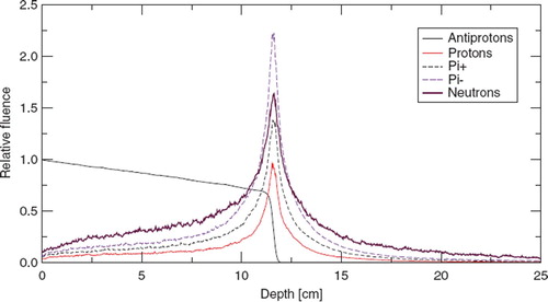
The multiplicity of neutrons originating from stopping beams of antiprotons in various media was experimentally investigated by Polster et al. [8], where the neutron energy spectrum was also characterized. From this reference it is possible to estimate that about 2 neutrons with energies above 1 keV are emitted per antiproton annihilation on a carbon ion. The neutron fluence calculated with FLUKA is approximately twice that of the antiproton fluence found in the annihilation peak, and dominates the fluence spectrum a few cm beyond the annihilation peak. Absolute neutron multiplicities from fast neutrons were also investigated by the AD-4 collaboration using neutron bubble detectors [9], and were found to be in agreement with Polster et al. [8], if accounting for the fact that the detectors used in the aforementioned reference also are sensitive to protons and pions. Still, we feel the need for an additional benchmark of the particle Monte Carlo code FLUKA for neutron production and transport. This is motivated by the discussion of the risk of secondary cancer induction by neutrons, which have very high relative biological effectiveness according to [10], especially at low dose. Currently this is the subject of active investigations for other particle beam therapy modalities, and several detailed studies have been published during the last several years [10–12].

The individual components of the mixed particle-energy spectrum emanating from the antiproton annihilation vertex have different ranges. Most nuclei have short ranges of a few mm from the annihilation vertex, but light particles with high energies like protons, pions, neutrons, as well as photons contribute to the dose in the peripheral region. Charged pions and photons interact only weakly with the target atoms and have ranges long enough that they can mostly escape the patient. Thus, in a treatment situation, they would leave the body with little interaction. Also these are believed to exhibit low-LET properties similar to those of protons [13]. The pion spectra shown in e.g. [14] indicates that most pions will have energies well above 40 MeV. Since pions have the similar stopping power as protons, if one calculates the energy in MeV per nucleon mass, a 40 MeV pion will have the similar range as a 270 MeV proton, which is 44 cm in polystyrene, using the continuous slowing down approximation (CSDA). Neutrons on the other hand, are moderated by the phantom body to lower energies, and are therefore in this context considered to have an intermediate range. Less energetic protons and light nuclei emerging from the annihilation vertex, have a shorter range, but the most energetic ones are still expected at a distance of roughly 3 cm from the annihilation vertex inside a polystyrene phantom (Figure 1) and are partially also discussed in [9]. In this paper we will show results from fluence determination experiments, which are aimed at characterizing the thermal neutrons found in the peripheral field inside a polystyrene phantom. The results are compared to Monte Carlo simulations and put in perspective with available literature on this subject.

Experimental Setup – Measuring Neutron Fluence with Thermoluminescent Detectors

Fast neutrons emerging from the antiproton annihilation vertex were studied earlier with bubble detectors and the results are described in [9]. As mentioned therein, the measurements were complicated by the fact that the bubble detectors also responded well to protons and presumably to pions, complicating the signal analysis. Therefore we designed a new experiment where we measure the thermal neutron fluence using pairs of thermoluminescent detectors (TLDs). We have used Mg,Ti doped LiF pellets consisting of either ⁶LiF or ⁷LiF, aka. TLD 600 or TLD 700 respectively. TLD 700 pellets are insensitive to thermal neutrons, whereas TLD 600 has a high cross section for thermal neutrons. In a radiation field where neutrons are present, an increased dose is expected to be seen in ⁶LiF TLDs relative to ⁷LiF, arising from the thermal neutron reaction ⁶Li(n,α)³H. Usually, TLD pairs are used in so-called Bonner spheres (see e.g. [15]), where various parts of the neutron energy spectrum can be thermalized and measured. The neutron energy spectrum from antiprotons annihilating on carbon is described by Polster et al in [8], and is a continous function which ranges from thermal energies up to ∼200 MeV. Most neutrons are found below 10 MeV. 10 MeV neutrons will reach thermal energies after 15 cm of polystyrene following the Fermi age model described by Uhm [16]. Our polystyrene phantom can be regarded as being similar to a Bonner sphere in the sense that we place TLD pairs at several distances from the annihilation vertex. For a TLD, surrounded by several centimeters of e.g. polystyrene (corresponding to the mean thermalization path-length), the thermal neutron field is expected to be rather isotropic. This, however, is not the case for the TLD pair located close to the edge of the phantom. In addition, the TLDs do not have a spherical symmetrical geometry, but are flat disks, being opaque to thermal neutrons. Hence, the orientation of the TLDs matters, when placed in a non-isotropic neutron field. This reduces the usability of the thermal neutron measurements for purposes other than benchmarking MC simulations or estimating the thermal neutron fluence at specific locations in the radiation field. All TLD pairs used in our experiment were calibrated at the Department of Physics and Astronomy at the University of Aarhus, Denmark in a thermal neutron field originating from a paraffin moderated Am-Be neutron source. Inside this paraffin block the thermal neutron fluence is well known and regulary checked for student excercises. We have irradiated three TLD 600 and three TLD 700 TLDs for 1 hour at 23000 neutrons/cm²/sec, in order to link the difference in TL response to the thermal neutron fluence.

TLD Handling Procedures

There are several ways of measuring the absorbed dose in TLDs. Measuring the thermoluminescent yield as a function of time, while increasing the heat at a constant rate will produce a glow curve, which reflects de-trapping of electrons and holes which recombine in thermoluminscent centers. The glow curve consists of several peaks, where each peak is related to a distinct trap level depth. One way of measuring the thermoluminscent (TL) signal is simply to integrate the light emitted by the TLD while heating up to e.g. 350 °C. When doing so, effects from fading of short lived shallow traps producing low temperature peaks should be considered, otherwise the integrated thermoluminescent (TL) yield may be less than expected. As a mitigation, the TLD which is about to be read out, can be pre-annealed, in order to reduce the light emitted from the low temperature glow peaks with short half-lives and thereby reducing the short term effect of fading. Pre-annealing of a TLD is usually done by maintaining the TLD at 100 °C for some minutes, before starting the readout cycle. Also, the individual glow curve peaks may show varying behaviour for different LET. For instance peak 6, here found at 564 K, is reported to show a LET dependence, being more sensitive to high-LET radiation than peak 5 [17,18], found at 497 K. To reduce the LET dependence of a TLD, one can integrate the thermoluminescent yield only up to the onset of peak 6, instead of integrating over the entire TL region. Here, we decided to overcome these problems by applying glow curve deconvolution into distinct peaks, and then express all TLD results in terms of peak 5 yield. This method reduces the amount of free parameters of the TLD handling protocol, which may have an impact on the acquired results. All TLDs used here are procured from TLD-Poland². MTS-6 and MTS-7 TLDs are used as Harshaw TLD 600 and TLD 700 equivalent TLDs, respectively. They will be referred to with their Harshaw equivalent names from here on. The TLDs are 0.025 cm thick and have a diameter of 0.45 cm. All TLDs were read out at the Aarhus University Hospital, Department of Medical Physics, using a TOLEDO 654 TLD reader from Pitman Instruments. This TLD reader is modified with a microprocessor board, to allow different TLD reader heating cycles to be programmed. In addition, four extra output ports are available: 2 analog ports which can be programmed to deliver a signal proportional to either the temperature, the time elapsed or the glow curve signal. The other two outputs are digital outputs, which provide TTL pulses for either temperature, time elapsed, or the glow curve signal at a programmable rate, and are intended for use with a multi channel analyzer (MCA). The temperature output is not transmitting the actual temperature on the TLD, but the requested target temperature as a function of time. This introduces a lag in the system, which underlines the importance of fixing the TLD readout protocol before any calibration and measurements are made. We programmed the TLD reader to heat a TLD to 60 °C and pause there for 20 seconds (including the warm-up phase). Then the temperature increases with a heating rate of 1 °C per second up to 380 °C. The heating rate is chosen to be low enough to achieve a good peak separation, which eases the glow curve deconvolution as described in section 2.2. Still, the heating rate should be sufficiently high to achieve enough signal for the TLD reader not to lose its calibration.

TLD Glow Curve Deconvolution

Usually the probability of releasing a trap at a temperature T is described by the Bolzmann distribution:

where E is the energy depth of the trap, T is the temperature in Kelvin, k is Boltzmann's constant, and s is an arbitrary frequency factor depending on the respective lattice defect. From equation 1 it is possible to derive an intensity function describing the glow curve generated by a single type of trap. Assuming a single trap in the luminescent material, a negligible retrapping of the electrons released, and recombination of all released electrons in the luminous centers, the intensity is related to the amount of trapped electrons n(t) at time t during heating [19]:

Applying a constant heating rate β so that T = T_o + βt, equation 2 transforms into the so-called first-order kinetic equation [20]:

where n_o is the trapped electron concentration at time t = 0. This equation cannot be solved analytically, but Kitis et al. [21] applied a second-order approximation to a rewritten version of the integral to express the first-order kinetic glow peak as a function of three parameters only:

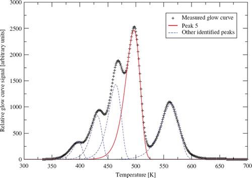
where I_m is the intensity maximum of a peak at the temperature T_m. Note, that the three parameters E, I_m, and T_m describe the width, height, and position of the peak, respectively. Δ = 2kT/E and Δ_m = 2kT_m/E. Several other glow-curve models exist as well, based on different assumptions than those mentioned above. The first-order kinetic model is a special case of the general one-trap (GOT) kinetic equation, as mentioned in Kitis et al. The GOT model also accounts for electron retrapping. In the limit that no significant electron hole retrapping takes place during the TL readout process, one obtains the first-order kinetics situation and equation 4 becomes a valid approximation. The second-order kinetics case occurs when the probability of retrapping is similar to the probability of light emitting electron-hole recombination. According to Levy [20] the first order kinetics function is applied for the “high dose” regime, whereas second-order kinetics are applied for “low doses”, without quantifying this closer. Here we merely observe that the first-order kinetics function yields credible fits to the glow curves from all our TLDs. Therefore the first-order kinetics model is used exclusively throughout this work, and thus the approximated intensity function presented in equation 4 is used to deconvolute the glow curve function. The area sum of each deconvoluted peak then corresponds to a certain amount of the absorbed dose for photon radiation. A glow curve deconvolution computer program is written, inspired by the CLEAN algorithm known from radio astronomy [22]. The above stated first-order kinetics function (eqn. 4), is the kernel function which is applied herein. The CLEAN algorithm is applied in order to get initial guesses for the position and amplitude of the peaks found in the glow curve. Here, we first locate the global maximum in the entire glow curve. This is usually the so called “peak number 5” found at around 500 K. I_m and T_m for this maximum are inserted in equation 4. E is always kept at a fixed value to reduce the amount of free parameters. (E was found earlier once from manual fits to the form of peak 5.) The calculated glow curve for peak 5 is then subtracted from the entire glow curve, and a new global maximum is found and again subtracted. This process is repeated until no new maxima above a certain threshold can be found. This table of initial guesses for I_m and T_m is then used for a parameter fit for the entire glow curve. To achieve the error bars of I_m, the fit is repeated a second time, but now only with I_m as a free parameter. Hence, the entire error of the glow curve deconvolution is expressed in the fitting error of I_m. Usually the error is less than 1% for peak 5. Finally, the result from the second fit is used to determine the areas of the individual peaks by numerical integration. Since more than a hundred TLDs were irradiated (including experiments not discussed here), the above stated deconvolution process was automated in a collection of scripts, reducing the workload significantly, and enabling fast deconvolution for possible future work. An example of glow curve deconvolution is shown in Figure 2.

Figure 2. Example of the automatic glow curve deconvolution for a TLD-700 equivalent pellet. The raw glow curve (“+” marks) is recorded a few hours after irradiation with 4 Gy of 6 MV X-rays. 5 peaks are deconvoluted in this example, but only the main peak at ∼500 K which is the so-called “peak 5” is used for further data processing.

TLD Calibration

All TLDs used in the experiment were calibrated using photons. Every single TLD is exposed to the 6 MV photon field of a medical linear accelerator. The accelerator is calibrated and its perfomance is checked with regular quality assurance procedures using absolute ionization chambers. The TLDs are covered with a few cm of solid water as a buildup material to achieve radiation equilibrium. The required dose was translated to monitor units and requested from the linear accelerator control system. The individual thermoluminescent signal (TL) from the calibration, TL_c, is then used as a reference for any other measurement afterwards. Instead of expressing the TL signal of a measurement in terms of arbitrary units, it is expressed in terms of a dose equivalent D_eq,γ [GyE] related to the calibration:

where D_c,γ is the dose applied at the TL calibration. Here we use the dose equivalent GyE term in order to discern between actual dose [Gy] and signal equivalent response, since the response per dose unit may change when exposed to high-LET radiation, which we except to be present in the neutron field. Since the calibration is done individually for each tablet, effects due to mass variations cancel out. Effects from light attenuation through the LiF material are considered negligible, since the LiF tables used here have a thickness d of 0.25 mm. The light attenuation through the TLD is described by Majborn et al. in [23] where a light absorption coefficient of μ = 2.38 cm⁻¹ is reported for their TLD 700 tablets. μ may vary depending on the crystalline structure of the TLD. Horowitz et al. [24] find μ = 1.8 cm⁻¹. In both cases the light attenuation is less than 3%. Here, the total light attenuation is not critical itself, as it would cancel out via the calibration, as long as the irradiation of the TLD can be considered aproximately equal from either side.

Phantom

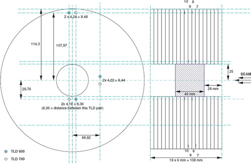
The phantom holding the TLD pairs is basically a hollow cylindrical block consisting of several slabs of polystyrene, as shown in Figures 3 and 4. Each slab can hold three pairs of TLDs, at three distances from the center axis. The entire phantom consisted of 18 slabs, but only four of the slabs were populated with TLD pairs, i.e. 12 TLD pairs in total. Each TLD pair consisted of one ⁶LiF TLD and one ⁷LiF TLD. The overall dimensions of the phantom resembles a typical human head. This configuration was subjected to a narrow beam of antiprotons twice: Once with a cylindrical polystyrene block inserted as a target to stop the antiproton beam in the center of the phantom, and once without a target so the beam could pass through the phantom unhindered, for background measurements. Also visible in Figure 3 is the aluminum block holding the white polystyrene phantom. The aluminum block has a 3 cm diameter central hole for the beam to pass unhindered.

Figure 3. The AD-4/ACE beam line at the antiproton decelerator at CERN with the thermal neutron phantom (the white plastic cylinder seen on the right). The antiproton beam enters the phantom from the left. Also seen on the image is the aluminum block holding the phantom. It has a hole which can let the beam pass unhindered. The box in front of the alumium holder, contains a thin scintilator foil which is monitored by a CCD camera (mounted at the top of the slant tube).

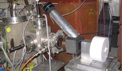
Figure 4. Technical drawing of the polystyrene neutron phantom, as seen from the beam (left) and from the side (right). On the right side, also the polystyrene annihilation target is shown in the center of the disks. The TLDs are located in disk number 7, 8, 9 and 10, counting downstream the beam direction. All dimensions are in mm.

Antiproton Beam

For irradiation we used a 300 MeV/c antiproton beam which corresponds to a kinetic energy of about 47 MeV, resulting in a range of about 2 cm in polystyrene. The beam profile was measured using GAF-chromic film and was determined to be gaussian with a FWHM of about 1 cm. A beam current transformer was used to measure the total number of antiprotons ejected to our experimental setup. Before entering the polystyrene phantom, the beam passes a scintillator foil which is being monitored with a CCD camera (also visible in Figure 3 as the box left to the aluminum block holding the polystyrene phantom). The antiproton decelerator (AD) at CERN delivers a spill of 3 • 10⁷ antiprotons every 90 seconds.

Experimental Results

The resulting background subtracted and calibrated TLD responses from this experiment are shown in Figure 5. For weakly interacting radiation, a r∼² dependence is expected since little attenuation (other than the inverse square law) happens. This is valid for both photons and pions. The pions from the annihilation vertex are expected to have a high energy. According to [14], most pions are found in the 100-300 MeV region, and apart from making the phantom transparent for them, this energy also leads to the estimated TLD response of approximately unity [18], again assuming that at these energies pions behave similar to protons. The upper plot in Figure 5 shows the individual and calibrated response of the TLD detectors, expressed in D_eq,γ. A kr⁻² curve fit was done to the TLD 700 set at 70 and 110 mm, and k was found to be 0.124 GyE mm² per 10 antiprotons. The measured trend is in good agreement with the inverse square law with the exception that the set at 30 mm exhibits a slightly larger signal. This may be attributed to the presence of protons, which most likely are still capable of reaching this detector set. The error bars are again a superposition of the error from the glow curve deconvolution and an estimated 5% inter-variability error resulting from the read-out procedure.

Figure 5. Top: ⁶LiF and ⁷LiF responses as a function of distance to annihilation vertex. k = 0.124 GyE mm². Bottom: difference in TLD 600 and TLD 700 responses in terms of thermal neutron fluence. a₀ = 2.86 · 10⁵. All results are absolute measurements expressed per 10⁷ antiproton annihilation. Error bars do not include a possible systematic underestimation of up to 20%.

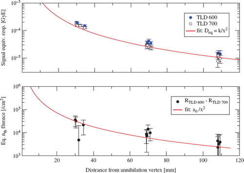
Using the Am-Be calibration, the response difference between ⁶Li and ⁷Li can be used to calculate the corresponding thermal neutron fluence. This measurement is an absolute measurement, since the result is expressed in terms of measured thermal neutron fluence per 10⁷ antiproton annihilations. The number of antiprotons hitting the phantom is not precisely known, since the antiproton count is done at a beam pickup well upstream the AD-4 beam line. Investigations indicate a possible loss of 10% percent of the beam measured at this point by the time it reaches the annihilation target. Additionally, the calibration of the beam pick-up occasionally revealed variations from year to year by about 10%. This could result in a possible systematic error of order 20% not reflected by the error bars in Figure 5. The experimental results are presented in table 1 below. In spite of the complicated nature of neutron moderation, an a₀r⁻² curve was fitted to the data to obtain a coarse estimation of the neutron fluence as a function of distance from the annihilation vertex. α₀ was found to be 2.86 · 10⁵ using a x² weighted fit to the data shown in Figure 5. It must be stressed that this curve has no foundation in any physical consideration.

Table I. Measured response of TLDs expressed in dose equivalent signal.

	[GyE] per 1e7 primary antiprotons
Position [mm]	TLD-600		TLD-600
30.0	1.99e-4	±1.56e-5	1.57e-4	±1.22e-5
30.4	1.87e-4	±1.48e-5	1.50e-4	±1.17e-5
32.0	1.55e-4	±1.36e-5	1.50e-4	±1.17e-5
34.5	1.50e-4	±1.23e-5	1.25e-4	±9.89e-6
69.0	3.52e-5	±4.95e-6	2.51e-5	±3.58e-6
69.2	3.73e-5	±5.48e-6	2.89e-5	±3.91e-6
69.9	4.17e-5	±7.88e-6	2.52e-5	±3.49e-6
71.1	3.48e-5	±5.51e-6	2.33e-5	±3.48e-6
108.0	1.28e-5	±3.65e-6	7.68e-6	±3.11e-6
108.1	1.50e-5	±3.85e-6	1.23e-5	±3.13e-6
108.6	1.45e-5	±4.14e-6	1.07e-5	±3.27e-6
109.3	1.41e-5	±4.02e-6	9.58e-6	±3.05e-6

Monte Carlo Simulations

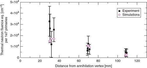
Based on excellent agreement with experimental measurements on antiproton beams achieved earlier [25,26] the MC particle transport code FLUKA 2008.3.7 [6,7] is used for Monte Carlo simulations of our set-up. During our simulations, the “HADRONTHE” default physics settings are used along with the “DPMJET-III” event generator [27]. The geometrical setup in FLUKA consists of the polystyrene phantom with 12 TLD pairs located as shown in Figure 4. An aluminum block serving to attach the phantom to the base plate of the AD-4 beam line is also included in the FLUKA simulations. The antiproton beam simulated is a 300 MeV/c beam with a momentum spread of 10 MeV/c and a divergence of 5 mrad. The radial profile is described by a Gaussian shape with a FWHM of 1 cm. For the results presented here, 5 · 10⁷ antiprotons were simulated. The result of the Monte Carlo calculation with FLUKA is compared with experimental results in Figure 6 and shows excellent agreement within the experimental error bars.

Figure 6. Measured and simulated thermal neutron fluence as a function of distance from the annihilation vertex inside the polystyrene phantom.

Discussion

The ⁷Li TLD measurements with the polystyrene phantom (with dimensions not unlike a human head) indicate a signal equivalent of (2.55 ± 0.18) · 10⁻⁵ GyE per 10⁷ antiprotons at a distance of 7 cm, for the contribution from photons and charged particles. The thermal neutron contribution at the same position yields a neutron fluence of (8.0 ± 2.4) · 10³ neutrons/cm² per 10⁷ antiprotons. The thermal neutron fluence can be translated to a kerma K [28]:

where [E(μ_tr/ρ)] is the neutron kerma factor. The thermal neutron kerma factor for an adult brain is 1.79 • 10⁻¹⁷ Gy m², according to ICRU 46 [28]. This yields a neutron kerma of about 1.4 · 10⁻⁹ Gy per 10⁷ antiprotons. Therefore, thermal neutrons themselves do not pose the major contribution to neutron dose in the body. It is instead expected that the primary contribution comes from fast neutrons. Additionally the neutron kerma factors increase with increasing neutron energy by about 2 orders of magnitude. For instance, at 1 MeV the neutron kerma factor for an adult brain is 2.58 · 10⁻¹⁵ Gy m². Initial calculations show, that a tumor of 1 liter ∼1 kg would require in the order of 10¹² antiprotons for 60 Gy(RBE) of target dose, assuming a field size of 10 × 10 cm², as well as an RBE of approximately 2 (RBE will decrease for larger SOBPs). Assuming 10¹² antiprotons, the contribution from thermal neutrons in terms of neutron kerma is about 100/μGy, which is low.

In contrast hereto, the measurements with the bubble detectors in [9] give an estimate of the fast neutron contribution, although for a different phantom. The reading of the bubble detectors are expressed in dose equivalent and is 12 mSv per 10⁷ antiprotons, or 1.20 Sv for 10¹² antiprotons, after subtracting the contribution from other charged particles. This was measured at a distance of roughly 8 cm from the annihilation vertex. The bubble detectors assume an isotropic field for the 1.2 Sv reading, as the unit Sv refers to the dose equivalent received by the entire body. The bubble detector measurements were made at a position close to a point-like source. Therefore this Figure may be misleading and additional modeling is still required to determine the dose equivalent.

Nonetheless, one may recall, that since the neutrons from antiproton annihilation arise from nuclear reactions induced by the pions, the neutron energy spectrum from a π⁻ beam is expected to be similar to that from antiprotons. For a comparison hereto, Vilaithong et al. [29] published calculations about the peripheral neutron dose from negative pion radiotherapy. Their estimations of absorbed neutron dose in tissue per stopped negative pion, is of similar magnitude as the bubble detector readings per antiproton, when using a weighting factor of 10 (see e.g. ICRP 60 [30]): Vilaithong et al. [29] find for a pion treatment dose of 50 Gy in a 1 litre treatment volume that the “total body” dose equivalent³ in this case is about 1.1 Sv, thus not unlike our 1.2 Sv per 1.0 liters for 60 Gy(RBE) target dose. Here they also assumed an RBE of 1.8 for the pions. The same group find a significant increase of neutron dose with treatment volume and speculate that this may limit the use of negative pions for therapeutic applications to tumor volumes smaller than 1 litre. Similar restrictions may need to be considered for antiprotons. Using the fit from the photon contribution measured with ⁷Li, one may calculate the photon/pion component. At 10 and 20 centimeter distance a TLD response equivalent to 1.24 GyE and 0.310 GyE can then be estimated, respectively, for 10¹² antiprotons.

Comparing passive proton beam delivery systems with antiproton therapy is rather pointless, since a passive system for antiproton would not only produce a large background dose but also be highly inefficient in delivering the rather precious antiprotons to the patient [31,32]. If ever an antiproton facility is to be build for medical applications, it must feature an active scanning system. Therefore comparisons of secondary radiation levels outside the target regions can reasonably only be performed using active beam scanning systems. In [12] a Figure with neutron dose equivalent (using the definition from [33]) as a function of distance is shown for proton beams, using both passive and active scanning systems. The active scanning data are partially based upon measurements made at the Paul Scherrer Institute in Switzerland. Schneider et al. [34] show neutron doses of about 2-3 mSv per treatment Gy at 10 cm distal from the beam central axis, which is one order of magnitude lower than what may be expected from antiproton irradation. For IMRT treatments the neutron doses are significantly lower, and the out-of-field equivalent dose is rather dominated by scattered photons [12]. According to ICRP 103 [5] the lifetime probability of developing a fatal secondary malignancy is about 5% per Sievert at low doses (i.e. below 100 mSv). Here we will not speculate further on the consequences for antiproton radiotherapy, since any further assesment of the neutron contribution to various organs will depend on the outcome of realistic treatment plans. Once this has been achieved, comparative studies of the stochastic effects of antiprotons versus other beam modalities can be undertaken as a next step, while using the here benchmarked Monte Carlo particle transport code.

Conclusion

We have performed measurements of the response of TLD detectors to the secondary particle spectrum resulting from antiproton annihilation. Using the difference between ⁷LiF and ⁶LiF detectors the thermal neutron fluence can be extracted. Results are in good agreement with model calculations using the FLUKA code version 2008.3.7. These results are also in general agreement with studies performed during the development of pion therapy in the 1980's. We find a low contribution from thermal neutrons, however the high substantial amounts of fast neutrons may still restrict antiproton therapy to smaller target volumes. The neutron exposure of the patient must be compared to the neutron background found in other particle beam therapy modalities like proton and carbon ion therapy. As these contributions are very system specific and vary widely with various delivery techniques a direct comparison may not be a valid approach and individual studies for each system my be more appropriate. Our findings indicate that FLUKA is well equipped to handle such questions, but idealy, a full neutron spectrum should be acquired using near clinical conditions.

Acknowledgements

The work was performed within the AD-4 collaboration and we are grateful to our colleagues for their support. The AD team worked diligently to provide the required antiproton beam and the beam diagnostics data necessary to obtain absolute results. The Danish Cancer Society and the ICE Center under The Danish Science Research Council supported this project with grants. MHH was supported in part by the National Science Foundation under grant CBET-0853157 and by the European Union through a Marie Curie International Incoming Fellowship grant PIIF-GA-2009-234814.

Declaration of interest: The authors report no conflicts of interest. The authors alone are responsible for the content and writing of the paper.

Notes

¹This calculation is for illustration purpose only, actual experiments described here were performed with a 47 MeV antiproton beam.

²http://www.tld.com.pl/

³In the reference simulated by a spherical shell with radii ranging from 6 to 26 cm.

References

- Holzscheiter MH, Agazarayan N, Bassler N, Beyer G, DeMarco JJ, Doser M, . Biological effectiveness of antiproton annihilation. NIM B. 2004;221:210–214.
- Holzscheiter MH, Bassler N, Agazaryan N, Beyer G, Blackmore E, DeMarco JJ, . The biological effectiveness of antiproton irradiation. Radiotherapy and Oncology. 2006;81:233–242.
- Experimental Studies Relevant for Antiproton Cancer Therapy. Aarhus University; 2006.
- Bassler N, Alsner J, Beyer G, DeMarco JJ, Doser M, Hajdukovic D, . Antiproton radiotherapy. Radiotherapy and Oncology. 2008;86:14–19.
- ICRP-103. Recommendations of the International Commission on Radiological Protection. The International Commission on Radiological Protection 2008. 103.
- Fassò A, Ferrari A, Ranft J, Sala PR. FLUKA: a multi-particle transport code; 2005. CERN-2005-10, INFN/TC_05/11, SLAC-R-773.
- Battistoni G, Muraro S, Sala PR, Cerutti F, Ferrari A, Roesler S, . The FLUKA code: Description and benchmarking. Albrow M, Raja R. Proceedings of the Hadronic Shower Simulation Workshop 2006. vol. 896 of AIP Conference Proceeding; 2007. 31–49. Fermilab 6–8 September 2006.
- Polster D, Hilscher D, Rossner H, von Egidy T, Hartmann FJ, Hoffmann J, . Light particle emission induced by stopped antiprotons in nuclei: Energy dissipation and neutron-to-proton ratio. Physical Review C. 1995;51:1167–1180.
- Bassler N, Knudsen H, Møller SP, Petersen JB, Rahbek D, Uggerhøj UI, . Bubble detector measurements of a mixed radiation field from antiproton annihilation. NIM B. 2006; 251:269–273.
- Brenner DJ, Hall EJ. Secondary neutrons in clinical proton radiotherapy: A charged issue. Radiotherapy and Oncology. 2008;86:165–170.
- Hall EJ. Intensity-Modulated Radiation Therapy, Protons and the risk of second Cancers. Int J Radiation Oncology Biol Phys. 2006;65:1–7.
- Xu XG, Bednarz B, Paganetti H. A review of dosimetry studies on external-beam radiation treatment with respect to second cancer induction. Phys Med Biol. 2008;53: R193–R241.
- Bassler N, Holzscheiter MH. Calculated LET spectrum from antiproton beams stopping in water. Acta Oncologica. 2009;48:223–226.
- Chamberlain O, Goldhaber G, Janeau L, Kalogeropoulos T, Segrè E, Silberberg R. Antiproton-Nucleon Annihilation Process. II. Physical Review. 1959;6:1615–1634.
- Hajek M, Berger T, Vana N. Passive In-Flight Neutron Spectrometry By Means of Bonner Spheres. Radiation Protection Dosimetry. 2004;110:343–346.
- Uhm HS. A theoretical model of neutron thermalization in a medium. J Appl Phys. 1992;72:2549.
- Schöner W, Vana N, Fugger M. The LET dependence of LiF:Mg,Ti Dosemeters and its applications for LET Measurements in mixed radiation fields. Radiation Protection Dosimetry. 1999;85:263–266.
- Horowitz YS, Satinger D, Fuks E, Oster L, Podpalov L. On the use of LiF:Mg,Ti Thermoluminescence Dosemeters in Space - a critical review. Radiation Protection Dosimetry. 2003;106.
- McKinlay AF. Thermoluminescence Dosimetry. vol. 5 of Medical Physics Handbooks. Adam Hilger Ltd; 1981.
- Levy PW. Thermoluminescence kinetics in materials exposed to the low doses applicable to dating and dosimetry. Nuclear Tracks and Radiation Measurements. 1985; 10:547–556.
- Kitis G, Gomez-Ros JM, Tuyn JWN. Thermoluminescence glow-curve de-convolution functions for first, second and general order of kinetics. J Phys D: Appl Phys. 1998;31:2636–2641.
- Högbom JA. Aperture Synthesis with a Non-Regular Distribution of Interferometer Baselines. Astronomy and Astrophysics Supplement. 1974 Jun;15:417.
- Majborn B, Bøtter-Jensen L, Christensen P. On the relative efficiency of TL phosphors for high-LET radiation. In: Proceedings of the Fifth International Conference on Luminescence Dosimetry; 1977. 124–130.
- Horowitz YS, Fraier I, Kalef-Ezra J, Pinto H, Goldbart Z. Non-universality of the TL-LET Response in Thermoluminescent LiF: the Effect of Batch composition. Phys Med Biol. 1979;24:1268–1275.
- Bassler N, Holzscheiter M, Knudsen H, the AD4/ACE Collaboration. Cancer Therapy with Antiprotons. Grzonka D, Czyzykiewicz R, Oelert W, Rozek T, Winter P. Low Energy Antiproton Physics-LEAP ′05. vol. CP796 of AIP Conference Proceedings. American Institute of Physics; 2005. 423–430.
- Bassler N, Hansen JW, Palmans H, Holzscheiter MH, Kovacevic S, the AD-4/ACE Collaboration. The Antiproton Depth Dose Curve Measured with Alanine Detectors. NIM B. 2008;266:929–936.
- Roesler S, Engel R, Ranft J. The Monte Carlo Event Generator DPMJET-III. Kling A, Barao F, Nakagawa M, Tavora L, Vaz P. Proceedings of the Monte Carlo 2000 Conference. Springer-Verlag Berlin; 2001. 1033–1038.
- ICRU-46. Photon, Electron, Proton and Neutron Interaction Data for Body Tissues. International Commision on Radiation Units and Measurements; 1991. 46.
- Vilaithong T, Madey R, Witten TR, Anderson BD, Baldwin AR, Waterman FM. Neutron doses in negative pion radiotherapy. Phys Med Biol. 1983;28:799–816.
- ICRP-60. Recommendations of the International Commission on Radiological Protection. The International Commission on Radiological Protection; 1990. 60.
- Paganetti H, Goitein M, Parodi K. Spread-out antiproton beams deliver poor physical dose distributions for radiation therapy. Radiotherapy and Oncology. 2010;95:79–86.
- Bassler N, Kantemiris I, Engelke J, Holzscheiter M, Petersen JB. Comparison of Optimized Single and Multifield Irradiation Plans of Antiproton, Proton and Carbon Ion Beams. Radiotherapy and Oncology. 2010;95: 87– 93.
- ICRP-26. Recommendations of the International Commission on Radiological Protection. The International Commission on Radiological Protection; 1977. 26.
- Schneider U, Agosteo S, Pedroni E, Besserer J. Secondary Neutron Dose During Proton Therapy Using Spot Scanning. Int J Radiation Oncology Biol Phys. 2002;53: 244–251.