Marginal Structural Models for Comparing Alternative Treatment Strategies in Ophthalmology using Observational Data

Treatment of many conditions in ophthalmology involves an extended sequence of decisions over a period of time. For example, in managing glaucoma, a target intraocular pressure (IOP) may be selected, and a topical eye drop prescribed, after which IOP is reassessed. If the IOP goal is not met using the one eye drop, another may be prescribed, and so on.1 Failure to adequately control IOP initially may lead to worsening of glaucoma as manifested by increased optic disk cupping and/or visual field loss, after which the target pressure may be revised further downward, and additional interventions considered. At each visit, a decision is made about whether or not to start a new treatment, or whether to stop an existing treatment. The goal of a clinician contemplating a series of decisions should be to choose the best available decision at each time or the best available strategy over time. Evaluation and comparison of such strategies using observational or non-experimental data is more difficult than the evaluation of simple one-time decisions or treatments, because of the complexities of characterizing the joint effects of a sequence of treatment decisions over time and adjusting for time-varying confounders in these settings.

The joint effects of a given series of treatments are evaluated with respect to a competing or comparison series as contrasts of what would happen under the different strategies.2,3 Even if one is interested in the effects of a single treatment among an extended series of treatments, it is important to avoid improperly attributing the effects of the treatment of interest to the effects of the other treatments in the sequence (each of which may be correlated with the treatment of interest). To accomplish these objectives, it is best to characterize these effects in terms of comparisons of treatment strategies which differ only at one point in time. In this editorial, we briefly describe these difficulties, present marginal structural models as an appropriate approach for dealing with them, and consider why some other popular methods are not appropriate for this setting.

Treatment strategies can be compared by a randomized trial in which each arm involves a different treatment strategy. For instance, the Multicenter Uveitis Steroid Treatment Trial compared a systemic versus a surgical implant strategy for non-infectious uveitis.4 However, it may not be feasible to conduct a randomized trial for every comparison of interest, particularly for less common diseases. In this situation, if evidence-based guidance is to be had, it is necessary to rely on observational data. When using observational data, one might think of simply comparing people who followed the different strategies, adjusting for confounding variables by using the standard approaches of regression adjustment or stratification for those confounders. This approach is problematic because of time-varying confounding variables affected by earlier treatment. Such variables have the following three characteristics2,3 (depicted in a causal diagram in Figure 1A): (1) they are independently associated with the outcome of interest – either because (1A) they cause that outcome, or because (1B) they share common causes with that outcome; (2) they are associated with the choice of subsequent treatment; and (3) they are affected by earlier treatment.

FIGURE 1. Causal diagrams depicting relationships among key variables, illustrating the issue of time-dependent confounding. (a) Actual relationships in a population, where the intermediate variable L is a time-dependent confounder. (b) Relationships in the pseudo-population created by weighting (condition 2 is removed). A_0, initial treatment; A₁, subsequent treatment; L, intermediate variable (disease activity); Y, outcome (visual acuity); U, common cause (possibly unmeasured) of L and Y. Conditions: (1) Covariate L is an independent predictor of outcome Y because of 1A (effect of L on Y) and/or 1B (unmeasured common cause U of L and Y). (2) Covariate L influences subsequent treatment A₁. (3) Covariate L is influenced by earlier treatment A₀.

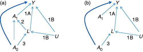
For instance, in the context of estimating the effects of treatment for ocular inflammatory disease, activity/severity of ocular inflammation likely plays this role. Because inflammatory activity is thought to be the major underlying cause of loss of visual acuity and most other adverse outcomes (condition 1A), observation of activity motivates the clinician to try a new (subsequent) therapy (condition 2), and is affected by prior treatment (condition 3). Elevated IOP in the context of glaucoma (see above) also may play this role, and several other examples may exist in ophthalmology. Characteristics 1A and 2 make the variable a confounder of the effect of subsequent treatment; to estimate that effect, one must adjust for the confounder. Characteristics 1A and 3 make the variable an intermediate on the causal pathway from earlier treatment to outcome.

It usually is inappropriate to adjust for a variable affected by treatment when one is attempting to estimate the treatment’s effect. For instance, in an observational dataset, it would be inappropriate to adjust for IOP after treatment when evaluating the effect of that treatment on the visual outcome of glaucoma cases. The reason for this is that when a variable (e.g. IOP) is an intermediate variable on the causal pathway (conditions 1A and 3), adjusting for it will produce biased estimates of the effect of the treatment of interest. If one tries to simultaneously estimate the effect of earlier and later treatments, adjusting by stratification or regression for an intermediate variable (e.g. IOP), the estimates of the effect of earlier treatment will be biased; the variable has characteristics 1A and 3 and so is an intermediate in the causal pathway by which a treatment has its effect on visual outcome (e.g. lower IOP may have a better visual outcome). However, if one tries to estimate the joint effects without adjusting for the intermediate variable (e.g. IOP), the estimates of the effect of the later treatment will be confounded, because characteristics 1 and 2 make that variable also a confounder which requires adjustment. Thus, in the presence of confounding by variables affected by prior and subsequent treatments (often known as time-varying or time-dependent confounders), standard analytic methods will be inappropriate.2,3

A fictitious illustration of these problems is given in Table 1. In this table, initial treatment decreases the proportion of subjects with increased IOP (condition 3); increased IOP both increases the probability of subsequent treatment (condition 2) and is associated with a higher probability of diminished visual acuity (condition 1A). Further, in this example, initial and subsequent treatment each reduce the probability of poor visual acuity by 10% within each subgroup. We performed standard regressions of diminished visual acuity simultaneously on treatment in both periods. When one does not adjust for IOP measured after the initial treatment, initial treatment is associated with a 10.7% decrease in poor visual acuity, whereas later treatment is associated with a 5.4% decrease. When adjusting for IOP, initial treatment is not associated with poor visual acuity, whereas later treatment is associated with a 10% decrease in poor acuity. Thus, neither regression correctly recovers the correct effects (10% reduction in the probability of poor visual acuity) of earlier and later treatments when both variables are included simultaneously in the regression models.

TABLE 1. Hypothetical data illustrating an observational study of the effect of IOP-lowering medication on visual acuity.

Initial use of IOP lowering medication (initial treatment status, A0)	Original population, n	Pseudo- population, n	IOP > 21 mmHg after A0 (intermediate variable, L)	Original population, n	Pseudo-population, n	Later IOP medication (subsequent treatment, A1)	Original population, n (%)	Pseudo-population, n (%)	Diminished visual acuity (%) (outcome, Y)
No	1000	4000	No	250	1000	No	200 (10.00)	500 (6.25)	35
						Yes	50 (2.50)	500 (6.25)	25
			Yes	750	3000	No	375 (18.75)	1500 (18.75)	55
						Yes	375 (18.75)	1500 (18.75)	45
Yes	1000	4000	No	750	3000	No	375 (18.75)	1500 (18.75)	35
						Yes	375 (18.75)	1500 (18.75)	25
			Yes	250	1000	No	50 (2.50)	500 (6.25)	55
						Yes	200 (10.00)	500 (6.25)	45

IOP, intraocular pressure.

The labels for the variables (A₀, A₁, L, and Y) refer to the corresponding labels in Figure 1. The pseudo-population represents what would have been seen had each person been able to participate simultaneously in each of the four arms of a clinical trial with treatment sequences no IOP medication-no IOP medication, no-yes, yes-no, and yes-yes; it essentially represents what might have been if IOP did not influence later treatment and so the effects of earlier and later treatment were un-confounded (note that initial treatment and IOP are associated with later treatment in the original population, column 5, but not in the pseudopopulation, column 6). In the weighted analysis, we simply regress the outcome on the treatment sequence, which is equivalent to the average in the weighted population of the outcome. Under the sequence no medication each time (“no-no”), this average is with diminished acuity. Similarly, the averages for the “no-yes,” “yes-no,” and “yes-yes” sequences are 40%, 40%, and 30%, respectively.

In response to this problem, Robins and co-workers developed a series of methods to estimate joint effects and model contrasts between treatment strategies in the presence of time-varying confounders: G-computation,5 G-estimation,6 and marginal structural models (MSMs).2,3 MSMs are the easiest to implement in practice, and so have become the method most commonly used to adjust for time-dependent confounding. MSMs typically are estimated using inverse probability of treatment weighting.2,3 The basic idea is to weight each subject by the inverse probability of receiving the treatment history that that subject actually had. This probability is computed from the probability of receiving treatment at each point in time given all that is known about that subject up to that time (i.e. prior covariates and treatment history). With the weighting, each subject stands in for himself or herself as well as all the subjects who fail to follow the same treatment history and who are otherwise comparable to that subject up until the time that their treatment history diverges from that of the index subject. The weighting process creates a pseudo-population in which prior covariate and treatment history are not associated with subsequent treatment, and so partially mimics a sequentially randomized trial in which treatment is randomized many times. The relationships among variables in the pseudo-population are depicted in Figure 1B; the approach removes the relationship between predictors of later treatment and treatment (Condition 2) and so removes confounding by those predictors. An example of how this is implemented is given in Table 1. Many standard regression programs (e.g. Stata and SAS) can perform weighted regressions. MSMs have been used in analysis of data in a variety of biomedical applications; their use for controlling confounding by time-varying variables often leads to substantially different and more plausible findings than more familiar methods.7

MSMs have their limitations. Unlike randomization, inverse probability weighting does not address the problem of unrecognized confounding due to unmeasured covariates. The approach thus requires that (1) the available covariates in fact do convey the information that was relevant to clinicians and patients in selecting the treatment that actually was used; and (2) that there is not enough unrecognized confounding to distort observed relationships. Thus, the inverse probability weighting only partially mimics randomized trials in that randomization addresses confounding not only by measured covariates but also by unmeasured ones.

Additionally, the weighting process can result in substantially increased uncertainty about treatment effects (wider confidence intervals) than standard regressions would when the latter are appropriate, increasing the probability of a type 2 error (false negative association result). This uncertainty can result from the fact that, in the weighted estimation, some subjects may have substantially lower weights than others. The increase in standard errors often but not always can be mitigated by using so-called stabilized weights;2,3 other strategies for dealing with large standard errors include weight truncation, which can induce bias.8 These problems with increased variance and some other problems also can be mitigated with G-computation and G-estimation, the other approaches to dealing with time-varying confounders; however, both currently are more difficult to apply than MSMs.

It is worth briefly contrasting MSMs with some other approaches which have become popular in recent years for similar problems. Propensity score adjustment9,10 is an appropriate approach to controlling confounding in simpler settings. However, standard propensity score adjustment cannot deal with confounding by variables affected by treatment and so is not appropriate for jointly estimating the effects of treatments given at multiple times when such confounding is present. Principal stratification11 provides a different approach for dealing with post-treatment variables but has not been used to define or estimate joint effects of a series of treatments in observational studies. Structural equations models, in their simpler forms,12 do not appropriately adjust for time-varying confounders. A more general version of structural equations models,12 not available in standard software, is essentially equivalent to G-computation.

As discussed above, the possibility of unmeasured confounders will prevent analysis of observational data using marginal structural models from displacing randomized clinical trials for key questions. However, the approach provides a much improved method for comparing alternative treatments in situations where clinical trials are not available but rich observational datasets are. Use of marginal structural models in this setting may improve substantially the quality of the evidence base available to guide treatment when clinical trials are not available or feasible.

Declaration of interest

The authors report no declaration of interest. The authors alone are responsible for the content and writing of this paper.

This study was supported primarily by National Eye Institute Grant EY014943 (Dr Kempen). Additional support was provided by Research to Prevent Blindness (RPB) and the Paul and Evanina Mackall Foundation. None of the sponsors had any role in the design and conduct of the report; collection, management, analysis, and interpretation of the data; nor in the preparation, review, and approval of this manuscript.

Financial disclosures: Marshall M. Joffe: Employment (E) University of Pennsylvania; Grant Funding (G) National Institutes of Health; Maxwell Pistilli: (E) University of Pennsylvania; (G) National Institutes of Health; John H. Kempen: (E) University of Pennsylvania; (Consultant (C)) Alcon, (C) Allergan, (C) Lux Biosciences, (C) Xoma, (G) EyeGate Pharmaceuticals, (G) National Institutes of Health, (G) Food and Drug Administration, (G) Lions Clubs International Foundation.

Contributions of authors: Conception and Design of the study (MMJ, JHK); Writing the Article (MMJ); Critical Review of the Article (MMJ, MP, JHK); Final Approval of the Article (MMJ, MP, JHK); Provision of Materials, Patients, or Resources (MMJ, JHK); Statistical Expertise (MMJ, MP); Obtaining Funding (JHK); Literature Search (MMJ); Administrative, Technical, or Logistic Support (MMJ, JHK).

Statement about conformity with author information: The material described in this paper is not research and therefore did not require institutional review board approval.

References

- Prum BEJ, Friedman DS, Gedde SJ, et al. Preferred practice pattern: primary open-angle glaucoma. San Francisco, CA: American Academy of Ophthalmology; 2010
- Hernan MA, Brumback B, Robins JM. Marginal structural models to estimate the causal effect of zidovudine on the survival of HIV-positive men. Epidemiology 2000;11:561–570
- Robins JM, Hernan MA, Brumback B. Marginal structural models and causal inference in epidemiology. Epidemiology 2000;11:550–560
- Kempen JH, Altaweel MM, Holbrook JT, et al. Randomized comparison of systemic anti-inflammatory therapy versus fluocinolone acetonide implant for intermediate, posterior, and panuveitis: the multicenter uveitis steroid treatment trial. Ophthalmology 2011;118:1916–1926
- Robins J. The control of confounding by intermediate variables. Stat Med 1989;8:679–701
- Robins JM, Blevins D, Ritter G, Wulfsohn M. G-estimation of the effect of prophylaxis therapy for pneumocystic carinii pneumonia on the survival of AIDS patients. Epidemiology 1992;3:319–336
- Suarez D, Borras R, Basagana X. Differences between marginal structural models and conventional models in their exposure effect estimates: a systematic review. Epidemiology 2011;22:586–588
- Cole SR, Hernan MA. Constructing inverse probability weights for marginal structural models. Am J Epidemiol 2008;168:656–664
- Rosenbaum PR, Rubin DB. The central role of the propensity score in observational studies for causal effects. Biometrika 1983;70:41–55
- Rubin DB. Propensity score methods. Am J Ophthalmol 2010;149:7–9
- Frangakis CE, Rubin DB. Principal stratification in causal inference. Biometrics 2002;58:21–29
- Pearl J. Causality: models, reasoning, and inference. 2nd ed. Cambridge: Cambridge University Press; 2009