Predicting changes in blood flow in patient-specific operative plans for treating aortoiliac occlusive disease

Abstract

Traditionally, a surgeon will select a procedure for a particular patient on the basis of past experience with patients with a similar state of disease. The experience gained from this patient will be selectively used when treating the next patient with similar symptoms. This article describes a surgical planning system that was developed to enable a vascular surgeon to create and test alternative operative plans prior to surgery for a given patient. One-dimensional and three-dimensional hemodynamic (i.e., blood flow) simulations were performed for rest and exercise for operative plans for two aorto-femoral bypass patients and compared with actual postoperative data. The information obtained from one-dimensional (volume flow distribution and pressure losses) and three-dimensional (flow, pressure, and wall shear stress) hemodynamic simulations may be clinically relevant to vascular surgeons planning interventions.

• Patient-specific
• hemodynamic simulation
• aortoiliac occlusive disease
• finite-element analysis

Introduction

Atherosclerosis is a degenerative vascular disease of clinical significance that leads to a narrowing of the flow lumen and, in more severe cases, prevents adequate flow to tissues and organs. In symptomatic patients with occlusive disease of the lower extremities, the infra-renal abdominal aorta and the iliac arteries are the most common sites of obliterative atherosclerosis [1]. Many patients asymptomatic under resting conditions experience ischemic pain under exercise conditions. The primary objective of a surgical intervention for aortoiliac occlusive disease is to restore adequate flow to the lower extremities under a range of physiological states including rest and exercise. Although volumetric flow distribution is of paramount concern initially following a surgical intervention, other quantities such as high particle residence time and low mean wall shear stress are theorized to be flow-related factors in disease progression and impact the long-term efficacy of a surgical intervention.

Several major classes of treatment exist for aortoiliac occlusive disease. One technique that may be appropriate for localized occlusive disease is to use catheter-based endoluminal therapies such as angioplasty and stenting. The use of angioplasty and stenting has received considerable attention recently because of probable cost savings and decreased morbidity when compared with traditional open surgical interventions. The most commonly used procedure for severe cases is direct anatomic surgical reconstruction and this is the focus of the work presented here. Direct surgical reconstruction refers to the insertion of grafts replacing or providing alternative pathways to flow through the infra-renal aorta and iliac arteries.

Currently, surgery planning for the treatment of vascular disease involves acquiring diagnostic imaging data to assess the extent of aortoiliac disease in a given patient. The surgeon then relies on his/her past experience, personal bias, and previous surgical training to devise a treatment strategy. Taylor et al. [2] proposed a new paradigm of simulation-based medical planning (SBMP) for vascular disease that involves using computational methods to evaluate alternative surgical options prior to treatment using patient-specific models of the vascular system. Blood flow (hemodynamic) simulations enable a surgeon to evaluate the flow features resulting from a proposed operation and to determine whether they pose potential adverse effects such as increased risk of atherosclerosis and thrombus formation.

Methods

There are several major steps in the SBMP process for vascular surgical applications [3–8]. First, patient-specific preoperative geometric models are created from medical imaging data by a technician. Additional imaging data may be needed to obtain physiological information. Next, geometric models representing several surgical alternatives to be evaluated are constructed under the guidance of the attending vascular surgeon. One- and three-dimensional numerical simulations are then performed on the different surgical interventions. Finally, clinically relevant analysis results are visualized and interpreted. This process can take a few hours to create preoperative geometric models and implement treatment plans, minutes to obtain flow and pressure results from the one-dimensional simulation methods, and several hours to obtain velocity, pressure, and shear stress results using the three-dimensional (3D) simulation methods.

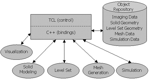
A modular software architecture has been developed as shown in Figure 1 to allow the use of best-in-class component technology and create a single application capable of surgical planning [3], [8]. Figure 1 shows three distinct parts: a front-end integration environment, a data repository for an abstract data exchange between modules, and modules roughly corresponding to the major tasks in the process. The remaining part of this section summarizes some of the important considerations.

Figure 1. Modular software architecture. Three distinct parts exist in the framework: a front-end integration environment (shown as a rectangle), an object repository (shown as a cylinder), and five modules (shown as ellipses).

Patient-specific geometric model construction and surgical planning

Magnetic resonance imaging (MRI) is a particularly useful imaging modality for SBMP because it can provide both physiological and 3D geometric information. In the case studies presented here, the medical imaging data were obtained using a GE Signa 1.5T MRI scanner (General Electric, Milwaukee, WI, USA). Ideally, the scanner creates linearly varying gradients of the magnetic field across the image volume. However, in practice, non-linearity of the magnetic field gradients exists, which must be accounted for or significant geometric errors will occur in the volumetric image data [9].

It is worthwhile pointing out the advantages and disadvantages of two- and three-dimensional image segmentation, because both are available in the system via an integrated multi-dimensional level set kernel [3]. For example, for small regions of interest with high signal-to-noise acquired with specialized surface coils (e.g., the carotid bifurcation), direct 3D reconstruction techniques are compelling. In contrast, in the case studies discussed herein, a body coil was used (because of the large extent of the vasculature required to model surgical interventions), reducing the quality of the acquired data. The presence of complex flow and significantly diseased vessels can cause poor signal and vessels only a few pixels in diameter in critical regions of interest (e.g., diseased common iliac arteries). The variability in the level of the contrast agent and noise in the image data can make the segmentation parameters a function of position. In addition, the human body contains a vast network of arteries, but it may be desired to simulate only a subset of them. It can be difficult to extract an accurate geometric representation using the level set method in 3D while preventing the front from advancing into undesired smaller branches (e.g., lumbar arteries). Finally, the one-dimensional simulation methods described in the next section require medial axis paths and circular cross-section segments. In any case, in vitro and in vivo animal validation studies have demonstrated that, despite the geometric approximations associated with using models lofted from two-dimensional curves, flow rates and velocity fields can be computed accurately using this approach [10–12]. Further discussion on possible improvements to the image segmentation may be found in the final section of this paper.

A detailed discussion of the methods used to construct preoperative geometric models from the MRA data can be found elsewhere [3], [4]. Briefly, a multi-stage process is used as shown in Figure 2. The first step involves extracting the medial axis paths for the vessels of interest, selecting points interactively or using a semi-automatic algorithm [13]. The 3D data are then sampled in planes perpendicular to the vessel paths at user-selected locations. Several segmentation techniques, including thresholding [14], interactively created contours, and level set techniques [15–18], can then be performed on the planar image samples to extract the lumen boundary. A solid modeling operation referred to as lofting is then used to create a 3D solid from the cross-sections of each vessel [19]. This consists of ordering and aligning the cubic splines created from the two-dimensional cross-sectional segmentations for a given vessel and creating a NURBS surface to represent the vessel wall where each segmentation is an isocurve on the underlying parametric map. A single 3D solid representing the flow domain is then constructed by Boolean addition (union) of the individual vessel solid models.

Figure 2. Overview of preoperative model construction. Initially, volumetric medical imaging data are acquired (a). Medial axis vessel paths are then extracted (b), followed by two-dimensional segmentation of the lumen boundary along each path (c). Solid models are then created for each vessel (d). Finally, the solid models representing the vessels are joined (Boolean addition) to create a solid model representing the flow domain (e). [Color version available online]

If a surgeon decides that a patient requires direct surgical revascularization and elects to perform an aorto-femoral bypass (AFB), three major design decisions are made to plan the procedure. First, the surgeon needs to select the type of graft (e.g., material, method of fabrication, etc.) and the appropriate size (e.g., standard sizes of bifurcated Dacron grafts include 14 mm × 7 mm, 16 mm  × 8 mm, 18 mm × 9 mm, and 20 mm × 10 mm). Inappropriate sizing can lead to inadequate restoration of flow or graft limb occlusion. The second decision is whether to use an end-to-end or an end-to-side proximal anastomosis [1]. Finally, the location, angle, and length of each distal anastomosis must be determined. Postoperative dilation of the graft, impact of graft coating such as Heparin, anastomotic aneurysm formation, thrombus, and hemodynamics of flow in the area of the anastomoses are areas of active research [20–26].

A surgeon can create a patient-specific surgical plan with the system using steps very similar to those used to construct the preoperative model. Specifically, for a direct reconstruction procedure, the surgeon defines the path(s) the graft will follow and the geometry of the graft flow domain by specifying elliptical and circular cross-sections that are lofted to create a solid model. The cross-sectional area specified should reflect the postoperative graft lumen diameter after implantation, i.e., after flow has been restored to the lower extremities. The degree of dilation is known to be device-specific [27].

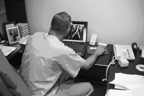
Although extensive research is underway in modeling, particularly with 3D geometric construction techniques, both balloon angioplasty and vascular stenting [28–33], the preoperative model construction process discussed previously allows for a straightforward first-order approximation of the stenting process. Specifically, when a lesion is identified, the surgeon can replace the actual contours in the affected region with idealized (circular or elliptical) segmentations that create an idealized lumen of the diameter and length of the stent(s). Figure 3 shows a vascular surgeon running the software developed as part of this work on his laptop computer to create a surgical plan.

Figure 3. The software system developed in this work was used by a vascular surgeon to create virtual surgical geometric models prior to the patient's actual surgery.

Boundary condition specification from PCMRI data

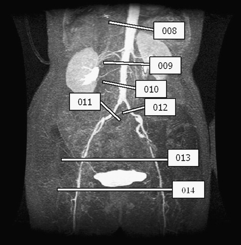
When MRA imaging data are acquired for the purpose of SBMP, planar slices of experimental data are also acquired, providing temporally and spatially resolved velocity fields (Figure 4). The technique used in the present work is known as cine-Phase-Contrast-Magnetic-Resonance-Imaging (PCMRI). PCMRI refers to a family of MR imaging methods that exploit the fact that nuclear spins that move through magnetic field gradients obtain a different phase than static spins, enabling the production of images with controlled sensitivity to flow [34]. With appropriate selection of imaging parameters, the technique can be used to quantify volumetric flow and provide insight into the spatial velocity fields in a given planar slice location [35].

Figure 4. PCMRI slice plane acquisition locations for 67-year-old female. Seven planes of through-plane velocity information were acquired at the locations shown in the figure.

Using PCMRI data to prescribe boundary conditions presents several challenges. First, the actual vessel deforms over the cardiac cycle. As the simulations used in this work rely on rigid-wall approximations, the temporally varying lumen must be mapped onto a rigid inlet surface as discussed later. Secondly, care must be taken when the volumetric flow from multiple PCMRI slices is used to prescribe various inlet and outlet flows. In reality, the net inflow of blood into the modeled vascular domain is equal to the net outflow. However, due to uncertainty and experimental error in the PCMRI data, it is often the case that the mean volumetric flow rates calculated from different slice locations are not conserved. In vivo, the instantaneous volumetric inflow is not required to equal the volumetric outflow because the vessel walls deform, providing a form of capacitance in the system. However, the incompressible rigid-wall approximation does enforce instantaneous conservation of mass.

If the experimentally determined velocity field is to be mapped directly onto the inlet of the model, it is typically required that the model be ‘trimmed’ at the location of the PCMRI plane. Initially, the geometric model is created to include the aorta proximal to the supra-celiac PCMRI slice plane location. This plane is then used to trim the solid model. Theoretically, the inlet surface of the model created by this trimming operation should correspond to the time-averaged cross-section contained in the PCMRI data. This is typically not the case, though, because of imaging limitations (spatial resolution, noise, partial volume effects, etc.).

Many of the applications of PCMRI to date have been for volumetric flow rate or volume fraction calculations [35]. The phase data experimentally acquired correspond to temporally discretized and spatially averaged velocity values in a given image voxel. For volumetric flow calculations, the volumetric flow is usually calculated with the through-plane velocity assumed to be a piecewise constant function. Although this is useful for volumetric flow calculations, the discontinuous nature of this representation is undesirable when creating velocity maps to be specified as the inlet boundary condition for a 3D hemodynamic analysis. If specifying velocity profiles directly from PCMRI data is desired, the software system developed as part of this work assumes that the velocity value is at the centroid of the voxel and uses bi-linear interpolation functions for each component of velocity to create a continuous representation of velocity [3].

As mentioned previously, in general, the lumen boundary in the PCMRI data is changing with respect to time. However, as rigid-wall approximations are being used, the temporally varying spatial velocity map from PCMRI needs to be mapped to the stationary inlet of the finite-element mesh. A simple mapping that assumes convexity of the lumen boundary and the inflow boundary of the finite-element mesh has been used in this work as discussed in reference 3. The mapping allows for rigid translation of the lumen in the PCMRI data with respect to the model constructed from the MRA data. However, any rotation between the two will contribute to error in the inflow boundary condition. An isotropic scaling is performed on the projected velocities to preserve volumetric flow rate. More sophisticated mappings may address some of the limitations of the current mapping strategy, although using mathematical models that account for wall deformability [36] seem more likely to improve the accuracy of the simulations.

It is often the case that one has only a volumetric flow rate and not a spatial velocity map such as the one provided by PCMRI data. This is typically the case for ‘small’ vessels, where insufficient spatial resolution of the PCMRI data does not yield a usable velocity field but does provide an approximation of the mean volumetric flow rate. In addition, mean volumetric flow through a vessel (e.g., the renal arteries) is often determined by taking slices above and below the branch location of the given vessel and using conservation of mass to calculate the unknown flow rate(s). In these cases, a useful approximation of the velocity field is given by assuming an analytic velocity profile as derived by Womersley for fully developed pulsatile flow of a Newtonian fluid in a rigid cylinder [37]. Note that, for even slight deviations from a circular cross-section or in the presence of insufficient length to generate a fully developed flow, this may be a poor approximation to the actual velocity profile.

PCMRI was acquired in the case studies presented here to quantify the volumetric flow through several arteries of interest. In addition to the relatively large (with respect to pixel dimension) arteries of interest such as the aorta, aorto-femoral reconstruction planning also requires the quantification of volumetric flow in small (relative to pixel dimension) and diseased vessels, such as the common iliac arteries. The software system described in reference 3 provides multiple segmentation and flow-calculating techniques needed for SBMP.

One-dimensional hemodynamic analysis

Postoperative volumetric flow distribution is of paramount clinical importance in alleviating the symptoms of claudication (i.e., inadequate flow to lower-extremity tissue). As discussed in reference 38, one-dimensional finite-element methods can be used to predict volumetric distributions and pressure losses. In addition to simulating resting conditions, volumetric flow distribution during exercise can be estimated by dilation and constriction of the distal vascular beds as described below.

With the assumptions that (1) blood flow velocity along the vessel axis is much greater than the flow perpendicular to the vessel axis, (2) blood can be approximated as a Newtonian fluid, and (3) the velocity profile along the axis is a scaled version of a parabolic cross-sectional velocity profile function, a non-linear one-dimensional equation for pulse wave propagation in elastic blood vessels has been derived [38]. The space-time finite-element formulation for solving the one-dimensional problem discussed in reference 38 has been integrated into the present software system (Figure 5). The major strength of the one-dimensional method is in its speed (CPU minutes versus CPU days for the 3D simulation described below). However, the disadvantage of the method is that it does not account for energy losses associated with secondary flows due to curvature, branching, stenoses, aneurysms, or complex 3D geometric features. As discussed in reference 38, minor losses due to pressure losses across a stenosis or branching can be incorporated to increase the accuracy of the one-dimensional method.

Figure 5. An example of the graphical user interface (GUI) of the system developed for surgical planning. The ‘Main Menu’ GUI guides a technician through the steps to go from medical imaging data to one- and three-dimensional hemodynamic simulation. The remaining windows in the figure are examples of controlling and running a one-dimensional analysis. [Color version available online]

An impedance boundary condition was used to simulate exercise [39], [40]. Briefly, a fractal-like tree, based on an input root radius, length-to-radius ratio, and asymmetric branching factor, was used to calculate an impedance function of time that produced reasonable physiological pressures and closely matched the preoperative flow distribution determined experimentally using PCMRI. By reducing the radii of the resistance vessels in the structured tree of the viscera and dilating those in the extremities, an outlet impedance approximating exercise conditions were obtained [39], [41].

Three-dimensional hemodynamic analysis

Mean wall shear stress and particle residence time are theorized to play an important role in disease progression. The patency of the bypass graft and long-term relief of the claudication symptoms are likely determined by flow features, which can only be determined from 3D analysis, whereas the one-dimensional analysis results provide estimates of flow distribution and pressure losses. In the 3D analyses presented here, due to current software limitations, it was assumed that the vessel walls were rigid and that blood behaves as a Newtonian fluid.

The geometric models were discretized using a commercial automatic tetrahedral mesh generator (Simmetrix, Inc., Clifton Park, NY, USA). Several of the advanced features of the meshing kernel were used in this work. Specifically, curvature-based refinement (mesh density in the area of larger curvature on the surface of the solid), model face refinement (mesh density specified on a model face), spatially based refinement (defining spheres or oriented right circular cylinders of mesh density in 3D space), and boundary layer meshing (highly anisotropic mesh refinement near the vessel wall) were used to increase the accuracy of the solution while reducing the overall number of elements. That is, by concentrating elements in regions of interest (e.g., stenoses), bifurcations, the outlets, and near the vessel wall, the quality of the numerical solution was improved while minimizing the computational cost of the simulation when compared with isotropic meshes of equivalent refinement. It should be noted that, although not explicitly used in this work, a postori error-based adaptive mesh techniques hold promise for automatically adapting the mesh to the error in the solution, further improving accuracy and reducing computational cost [42].

There are several options when specifying boundary conditions for rigid-wall 3D simulations. First, if the volumetric flow distributions are known, it is possible to specify the boundary conditions using assumed velocity profiles. In much of the authors' previous work [3], [5],[43–45], this was done by specifying Womersley analytic profiles with the desired volumetric flow rate at all the outlets of the flow domain, except for a single outlet where a constant pressure was prescribed. Conservation of mass will ensure that the flow through the zero-pressure outlet matches the desired volumetric flow rate.

However, in the case of SBMP, the postoperative flow distribution is not typically known a priori. A method commonly used (partially due to its wide availability in commercial flow solvers) to avoid explicitly specifying outlet flows is to prescribe zero pressure at all the outlets of the modeled flow domain. The flow distribution is then dictated by the geometry of the flow domain. In reality, however, the flow distribution is principally governed by the downstream vascular beds that are too small or extensive to be modeled directly from diagnostic imaging data. This can lead to significant errors even in simple model problems [46]. For this reason, Taylor and Hughes [47] proposed coupling zero- and one-dimensional models to represent the downstream domain. In addition to the methods employed in this work [46], several other approaches have been used successfully [48–51]. Although some have proposed prescribing volumetric outflow distributions assigned to the arteries based on the one-dimensional analysis results [6], in this work appropriate resistance values were calculated using a coarse mesh as described in the Results section.

A flow solver developed by Jansen and colleagues [52–54], extended by Vignon et al. [46], and based on a stabilized finite element method introduced by Brooks and Hughes [55] was used to solve the Navier–Stokes equations (see also reference 43 for additional details on the solution strategy). The meshes were decomposed using a domain decomposition algorithm [56], enabling calculations to be performed in parallel. Two machines were used: a 128-processor (400 MHz IP35 MIPS), 32-node SGI Origin 3800 supercomputer with 64 GB of shared memory, and a mini-cluster of five Shuttle XPC Windows XP-based personal computers (each with a Pentium IV 3.0-GHz processor, 800-MHz front side bus with 1-MB L2 cache, 2 GB of PC3200 DDR RAM, 250 GB of RAID 1 storage) connected via standard gigabit ethernet.

Hemodynamic visualization

The hemodynamic simulations yield hundreds of megabytes (often gigabytes) of analysis results. Scientific visualization transforms the millions of scalars and vectors produced during the analysis into visual images that can be used to understand the flow solutions [14]. The system used [3] directly integrates standard and application-specific visualization (i.e., postprocessing) capabilities directly relevant to surgical planning, as discussed below.

Three specific examples highlight the benefit of the integrated visualization environment provided by reference 3. First, the analysis results can be viewed directly inside the same window with the volumetric image data to provide additional anatomic context to the solutions. In addition, the user can specify the location of a cut plane on the basis of a PCMRI slice, enabling the direct comparison of finite-element results to experimentally acquired velocity results. Secondly, information used in the construction of the solid model can be used directly to query the analysis results. For example, the user can plot velocity and pressure along a medial axis path. Finally, additional functionality is integrated to calculate postprocessing quantities of interest such as wall shear stress.

A surgeon may want to review velocity profiles, pressure distributions, and scalar clearance time for a proposed surgical procedure. In addition, several postprocessed quantities are also of interest because of their theorized role in atherosclerosis. Specifically, instantaneous wall shear stress, mean wall shear stress, shear stress pulse, and oscillatory shear index (OSI) are all derived quantities of the solution of interest to a vascular surgeon.

Results

Two case studies demonstrate the application and limitations of the system for planning an aortofemoral reconstruction procedure. The first case involves a 67-year-old female patient, while the second case involves a 55-year-old male patient.

Case study of a 67-year-old female patient

A 67-year-old female with rest pain and calf claudication at 20 feet and with a past medical history significant for peripheral vascular disease (ankle brachial index 0.50 bilaterally), chronic obstructive pulmonary disease, nicotine abuse, and cerebral vascular occlusive disease (60% carotid stenosis) was studied. Non-invasive imaging was consistent with atherosclerotic occlusive disease of the iliac and femoral arteries bilaterally.

Imaging data were acquired preoperatively (Figure 6a) to obtain geometric information (using MRA) and quantify volumetric flow (using PCMRI) in the aorto-iliac–femoral system. Approximately 2 weeks after the acquisition of the preoperative data, the patient underwent an end-to-side aorto-femoral reconstruction. A Dacron bypass graft with nominal dimensions of 14 mm × 7 mm was used.

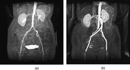
Figure 6. MIP of preoperative and postoperative MRA for a 67-year-old female. (a) The extent of the occlusive disease preoperatively (notice the tight stenosis in the patient's left external iliac) and (b) the bypass graft and the occlusion of the external iliac arteries postoperatively.

Postoperative image data were acquired ∼6 months after the operation (Figure 6b). The patient was symptom free at that time (i.e., she felt better than prior to the operation), although diagnostic imaging and testing indicated a progression of the disease. There was mild narrowing of the profunda femoris arteries distally, and the external iliac arteries that were bypassed had occluded completely.

Geometric modeling and operative planning

Prior to the patient's surgery, a preoperative geometric model and a postoperative geometric model of a direct revascularization procedure were constructed (Figure 7). However, for the retrospective study included in this paper, an improved geometric model was constructed for both the preoperative and postoperative models, using improvements in the software architecture and insight gained from subsequent model construction. As discussed below, a radiologist with expertise in reading MR images provided assistance in interpreting the preoperative MRA. In addition, to reduce the error of modeling the bypass graft dilation and location, a plan was created that was similar to the actual operation.

Figure 7. Two surgical alternatives for the 67-year-old female. (a) The preoperative model constructed prior to surgery. (b) A close-up of a high-grade stenosis in the left femoral artery. (c) The idealized endovascular repair (angioplasty and stenting), and (d) an aorto-femoral direct reconstruction using a Dacron bifurcating graft. [Color version available online]

Constructing geometric models for surgical patients presents significant challenges not found in volunteer subjects [15] and many in vivo validation studies [10]. In this particular case, the combination of a female patient with significant occlusive disease caused many of the vessels of interest to be small in relation to the resolution of the volumetric image data (in certain cases, only a few image pixels were seen across the diameter of the vessel). The image resolution and diffuse vascular disease led to three specific geometric modeling challenges discussed below.

The first geometrically challenging region, shown in Figure 8a, was proximal to the renal vessels in the abdominal aorta. It was initially unclear whether the celiac trunk, superior mesenteric artery, or both were patent. Although the image data showed what appears to be only a single vessel branching off from the aorta, it seemed plausible that two vessels could branch off very close to each other and blur together within the limitations of the image resolution. After a consultation with a radiologist, however, it was determined that only the superior mesenteric artery was patent and that it branched from the aorta in the region shown in Figure 8a.

Figure 8. Anatomic variability caused by vascular disease. The preoperative solid model is shown (in red) with three views created from the MRA data using thresholding. (a) The celiac trunk is not patent because of advanced vascular disease. (b) A dissection near the branch of the left internal iliac artery. (c) A tight stenosis that causes the vessel to appear disjoint because of the limitations in the image resolution and the threshold value selected. [Color version available online]

A second challenging area occurred near the branch point of the left internal iliac artery from the left common iliac artery (Figure 8b). Several different anatomical possibilities seem to exist to explain the imaging data shown. For example, this area could be an aneurysm (with flow recirculation causing a drop in signal intensity). It also could be a stenosis of the external iliac artery, with the left internal and external iliac arteries being ‘twisted’ around each other, making them appear as seen in the figure. Upon consultation with a radiologist and the attending vascular surgeon, it is believed that this region represents an ‘intimal flap’ causing limited flow in the ‘hole’ of the ‘donut.’ Given the difficulty of modeling this region using the lofting techniques described previously, and the fact that this region is removed from the areas of principal interest, it was approximated as a mild aneurysm in this work.

Finally, the imaging data made it difficult to ascertain the level of stenosis and patency of the left external iliac artery (Figure 8c). In the opinion of the surgeon, the external left iliac artery was severely occluded but patent. He estimated a 90% stenosis on the basis of other diagnostic imaging data, but a more conservative stenosis of 70% stenosis was used in the analyses presented here for meshing and numerical reasons.

For the AFB surgical plan, a geometric model was created similar to the actual operation. The objective was to use the knowledge and data gained from the postoperative MRA to create a plan as close as possible to the actual operation on the preoperative model. There is an important distinction between the procedure to be described and simply creating a model from the postoperative data. In particular, the external iliac arteries have completely occluded in the postoperative scan, making it impossible to build a model directly from the postoperative scan to study the flow in the external iliac arteries immediately following the surgical procedure. However, using the postoperative data, the dilation of the graft and the proximal take-off angle as a result of the actual surgery can be accurately modeled. To achieve an operative plan as similar as possible to the real surgery, the following steps were performed:

1. A preoperative model was constructed from the preoperative MRA data.

2. Three points were selected on the model (the location of the aortic bifurcation, the left internal iliac bifurcation, and the right iliac bifurcation), and the preoperative model was rigidly rotated into the same space as the postoperative MRA data.

3. Paths for the left and right limbs of the bypass were automatically extracted from the postoperative MRA data.

4. A surgical plan was constructed using the paths from step 3 as a guide. Specifically, the paths from step 3 were used explicitly until approximately the S/I coordinate of the internal iliac bifurcations. The paths then maintained the approximate shape of the real bypass but were extended and stretched, so that the bypass would intersect the preoperative model at the approximate S/I location of the distal anastomosis, as seen in the postoperative MRA.

Processing PCMRI data

MRI data were acquired in this case study to quantify the volumetric flow through several arteries of interest. Many previous studies have focused mainly on quantifying volumetric flow in the supra-celiac and infra-renal aorta in healthy subjects [57], [58], partially due to the large size of the aorta in relation to the in-plane image resolution. SBMP, however, also requires the quantification of volumetric flow in small (relative to pixel dimension) and diseased vessels, such as the common iliac arteries. In this case study, the vessels were roughly divided into three categories: large, medium-size, and small.

For large vessels (typically over 10 image pixels in diameter), the level set segmentation technique was used to determine the lumen boundary from the potential data. Figure 9 shows two representative frames of data from the supra-celiac aorta. The in-plane image resolution in this acquisition was 1.25 mm × 1.25 mm. This resulted in approximately 20 pixels across the lumen during peak systole in the supra-celiac aorta (Figure 9a). For medium-size vessels (roughly between 5 and 10 pixels across the vessel diameter), a threshold of the image intensity data was used to segment the lumen boundary. Finally, for small vessels with five or fewer pixels across the diameter, the individual pixels were selected and used in calculating the volumetric flow rate through the artery. This was done interactively, where the user can select an individual pixel in the image data and a volumetric flow waveform for that pixel will be displayed. The user then decides whether the waveform corresponds to what would be expected through the vessel of interest and includes the pixel if desired. This technique introduces significant user-dependence into the volumetric flow calculation because the inclusion/exclusion of a single image pixel can significantly alter the mean volumetric flow through a small artery of interest.

Figure 9. Two different time points of the supra-celiac aorta acquired using PCMRI. During peak systole (a), the supra-celiac aorta is approximately 20 pixels across and the lumen boundary is clearly visible in the zoomed view of the magnitude of the gradient plot (b). However, during parts of diastole, the lumen boundary is not as clearly defined, as seen in (c) and the corresponding zoomed magnitude of the gradient plot (d).

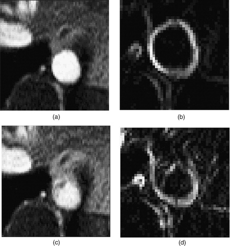
It should be noted that even for major arteries with 20 image pixels across the diameter, the lumen boundary is not always well defined. For example, a selected image frame from diastole in the supra-celiac aorta (Figure 9c) shows the ambiguity that can occur. The potential data at this time point do not clearly define a lumen boundary. While the software provides several options for creating lumen boundaries that may be applicable to this type of situation, the predominant technique used here was to copy segmentations from previous frames in the cardiac cycle where the boundary was well defined. This assumes the vessel does not change significantly between time points in the PCMRI acquisition, which may be reasonable given the increased rigidity of diseased vessels such as the ones studied here.

For this case study, seven slices of PCMRI data were acquired preoperatively, as shown in Figure 4. During acquisition, the plane locations are selected to be perpendicular to a given vessel of interest. Only the through-plane component of velocity was acquired to improve the temporal resolution of the data. As discussed elsewhere [35], a common postprocessing technique used to eliminate the effects of eddy currents leading to erroneous velocity in otherwise stationary tissue is known as ‘baseline correction’. Differences in lumen segmentation and user-selected regions for baseline correction can have a significant impact on mean volumetric flow rate [3]. For the purposes of this work, baseline correction was not used. Postoperative PCMRI data were acquired 6 months after the operation, at the same time as the postoperative MRA data shown in Figure 6b. The segmentation and processing issues are similar to those described previously. Table I summarizes the preoperative PCMRI data and Table II summarizes the postoperative experimental data.

Table I.  Mean volumetric flow rate, vessel cross-sectional area, and diameter from PCMRI data.

Series*	Location	Mean volumetric flow (ml/min)	Mean area (mm^2)	Effective diameter (mm)
8	Supra-celiac aorta	2247	417.97	23.07
9	Infra-renal aorta	796	110.30	11.85
10	Supra-bifurcation	716	109.00	11.78
11	Right common iliac	320	39.30	7.07
12	Left common iliac	400	45.10	7.58
13	Right infra-internal iliac	263	29.70	6.15
13	Left infra-internal iliac	214	20.30	5.08
14	Right femoral	148	20.30	5.08
14	Left femoral	119	12.50	3.99

*Refer to Figure 4.

Table II.  Mean volumetric flow rates from postoperative PCMRI data.

Location	Mean volumetric flow rate (ml/min)
Supra-SMA	2171
Infra-renal supra-bypass	492
Right common iliac	90
Left common iliac	113
Bypass body	230

Although the PCMRI data provide insight into the flow in the supra-celiac and infra-renal aorta, they do not provide information on the flow split between the superior mesenteric artery and the renal arteries. For the numerical simulations, however, flow distributions at each outlet are needed. As the patient represents abnormal (i.e., diseased) anatomy, standard flow distributions found in the medical literature [59] are not directly applicable. For the purposes of this study, it was assumed that flow lost between the supra-celiac slice and the infra-renal slice was divided as follows: 50% in the superior mesenteric artery and 25% to each renal artery. In addition, the patients' blood pressure during the MR acquisition was not acquired, so a physiologically reasonable mean pressure of ∼100 mmHg was assumed and used as discussed below.

Three-dimensional hemodynamic simulation

For the 3D simulations, as the primary quantities of interest were postoperative flow distributions, constant resistance boundary conditions [46] were employed for simplicity. That is, the pressure and volumetric flow rate at each outlet of the model were related via a constant resistance given by the equation (analogous to Ohm's law for circuit analysis):where P (t) is the pressure at a given outlet as a function of time, Q (t) the volumetric flow rate at a given outlet as a function of time, and R the constant to match the experimental data.

As only the desired mean volumetric flow rate is initially known, a simple iterative procedure was used. A coarse mesh of the preoperative geometric model consisting of 263,349 elements (56,282 nodes) was constructed. An initial guess of the outlet resistances was made, assuming the mean outlet pressures were uniformly 100 mmHg, by R = P_mean/Q_mean. This simulation was then run for three cardiac cycles (to achieve periodicity in the solution due to inexact initial conditions). The mean pressure on each outlet was then calculated from the finite-element solution, and an updated resistance value (using the desired flow rate and the current mean outlet pressure solution) was derived. This new resistance was then used for an additional simulation, and so forth until the discrepancy between desired mean volumetric and actual volumetric flow rate fell below a desired error threshold. After four such iterations, the maximum error in mean volumetric flow rate was less than 2.5%, so the resistances were assumed to be adequate for surgical planning purposes. Table III summarizes the iterations.

Table III.  Iterations to calculate resistance values for three-dimensional simulation to match target mean volumetric flow distribution.

Vessel	Target flow rate (ml/min)	Volumetric flow rate (ml/min)				Deviation from target mean flow rate (%)
		Sim 1	Sim 2	Sim 3	Sim 4	Sim 1	Sim 2	Sim 3	Sim 4
Supra-celiac	2247	2247	2247	2247	2247	0.0	0.0	0.0	0.0
SMA	725	662	706	717	719	−8.7	−2.7	−1.2	−0.8
Left renal	363	385	364	357	354	6.3	0.4	−1.6	−2.3
Right renal	363	339	361	366	366	−6.5	−0.6	0.8	0.9
Infra renal	796	860	816	808	807	8.0	2.6	1.5	1.4
Left common iliac	392	408	396	397	398	3.9	0.9	1.2	1.4
Right common iliac	404	451	422	413	410	11.9	4.5	2.3	1.5
Internal left iliac	182	216	190	186	185	18.4	4.1	1.9	1.6
Internal right iliac	146	170	152	149	148	16.9	4.2	2.0	1.4
Left femoral	210	192	206	211	212	−8.7	−1.8	0.5	1.2
Right femoral	258	281	270	264	262	9.0	4.6	2.5	1.5

Sim = simulation.

After the resistances are known, and given the inflow waveform from PCMRI shown in Figure 10, simulations of the surgical alternatives at rest were performed. A refined mesh for the preoperative model (621,679 elements with 124,758 nodes), AFB model (410,742 elements with 85,859 nodes), and PTA and stented model (632,713 elements and 126,788 nodes) was created. Figure 11 shows a representative mesh of the AFB operative plan. Blood flow simulations were performed assuming a blood viscosity of 0.04 poise and density of 1.06 g/cm³ for three cardiac cycles with 600 time steps per cardiac cycle. Convergence studies in reference 3 suggest that these are reasonable values for mesh density, time-step size, and number of cardiac cycles to achieve periodic solutions. Table IV summarizes the flow results at rest for the preoperative mode and two different surgical interventions. As mentioned previously, the 3D solutions provide additional potential quantities of interest, including wall shear stress. Figure 12 shows a representative mean wall shear stress plot for the preoperative model at rest and Figure 13 shows the mean wall shear stress plot for the AFB surgical plan. In addition to wall shear stress, particle residence time is theorized to play a part in disease progression. To gain some insight into particle residence time, a scalar clearance-time simulation has been performed. Conceptually, an initially uniform dye is passively advected by the flow and allowed to diffuse into the domain. When run over several cardiac cycles, areas of low flow tend to maintain a higher concentration than surrounding areas of higher flow. Figure 14 shows an example of a dye-clearance simulation for the AFB operative plan [3]. Notice that the external iliac arteries have significantly higher concentrations of dye compared with the native aorta and the bifurcating bypass graft after several cycles. As discussed in greater detail below, the simulation results could explain the clinically observed occlusion of the external iliac arteries postoperatively.

Figure 10. Rest and exercise supra-celiac flow waveforms for the 67-year-old female. The rest flow waveform was experimentally acquired using PCMRI. The exercise flow waveform was generated by shortening the diastolic portion of the rest curve by one-third and scaling the mean volumetric flow rate by a factor of two.

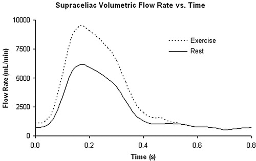
Figure 11. Exterior surface mesh for the model of the 67-year-old female patient. The mesh consists of 1.8 million tetrahedral elements.

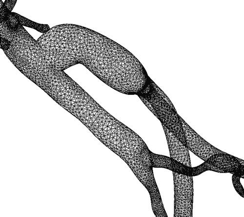
Figure 12. Mean wall shear stress for preoperative model. (a) shows the mean wall shear stress for the entire preoperative model. (b) shows a zoomed anterior view of the infra-renal aorta, while (c) shows a posterior view of the infra-renal aorta. Notice the region of low mean wall shear stress located just proximal to the aortic bifurcation, an area predisposed to atherosclerosis.

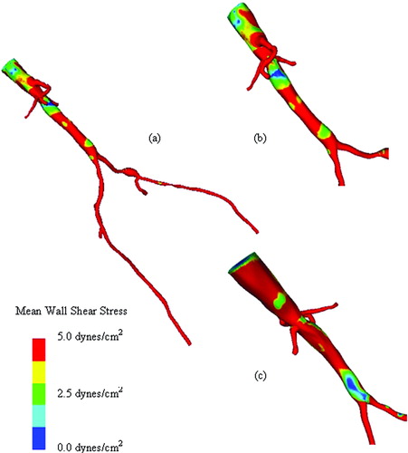
Figure 13. Mean wall shear stress for AFB model. Regions of low mean wall shear stress (shown in blue) are theorized to be sites of high risk for the development of atherosclerosis or neointimal hyperplasia.

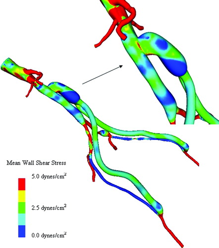
Figure 14. Scalar clearance time for AFB model. (a) The scalar field is initially set to 1.0 (shown in red) with a zero scalar Dirichlet boundary condition at the inlet. The scalar is then advected and diffused out of the flow domain over several cardiac cycles (where time is increasing from (a) until the final time point shown in (d)). The vessel walls have a scalar flux of zero.

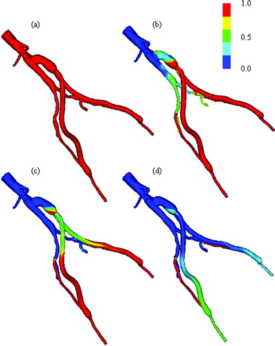
Table IV.  Comparison of mean volumetric flow rates from three-dimensional simulations of rest and exercise.

Location	Rest			Exercise
	Preoperative (ml/min)	AFB (ml/min)	Stent (ml/min)	Preoperative (ml/min)	AFB (ml/min)	Stent (ml/min)
IR aorta (proximal bypass)	792	888	837	3472	3901	3660
Bypass body		555			2340
IR aorta (distal bypass)		333			1564
Bypass right limb		247			1098
Bypass left limb		306			1243
Right external iliac	258	14	248	1107	73	1053
Left external iliac	208	2	276	527	− 23	907
Right femoral	258	262	248	1107	1171	1053
Left femoral	208	309	276	527	1221	907

Simulating exercise conditions

In addition to resting conditions, the benefit of an intervention due to mild exercise (e.g., walking) is of clinical significance. As discussed in the Methods section, Steele et al. [39] proposed that constricting the final generations of branches of the fractal trees in the viscera and dilating the vessels of the peripheral arteries can simulate exercise conditions. Given the outlet resistances calculated previously and the root radius of the fractal tree (given by the outlet diameters of the geometric model branch), an inverse iterative calculation can be performed to calculate a given length-to-radius ratio for the fractal tree. As exercise flow data were not collected for this patient, the values for constriction of the viscera (0.7) and dilation of the periphery (5.0) proposed by Steele et al. [39] for healthy young subjects were used. Given the length-to-radius ratio, inlet radius of the fractal tree, and dilation and constriction factors, the resistance of each branch can be calculated. The zero-order frequency mode for rest and exercise at the model outlets is summarized in Table V.

Table V.  Zero frequency mode of impedance boundary conditions at outlets for rest and exercise.

Vessel outlet	Root radius (cm)	Length- to-radius ratio	Z(0) rest (dyne*s/cm^5)	Z(0) exercise (dyne*s/cm^5)
Right femoral	0.202	40.34	36277	6197
Left femoral	0.203	34.37	30460	5739
SMA	0.192	10.07	10365	33049
Left renal	0.157	15.35	26393	85335
Right renal	0.154	11.59	21027	68957
Left internal iliac	0.257	115.28	55029	11726
Right internal iliac	0.159	41.49	68649	10550

As the exercise flow data were not collected, an inlet waveform for exercise had to be created. Although studies have shown a 2.4-fold increase in abdominal aortic flow during exercise for healthy female subjects maintaining a 150% increase in heart rate [60], [57], as a conservative estimate, given the diseased state of the patient, a 2-fold increase in supraceliac flow was assumed. For the simulations in this study, the length of the diastolic portion of the flow-rate curve was shortened by one-third and the entire waveform was scaled to increase the mean volumetric flow rate by a factor of two. The new waveform is shown in Figure 10. The flow during simulated exercise can be found in Table IV.

One-dimensional hemodynamic simulations

In addition to the 3D analyses discussed previously, one-dimensional analyses were performed for the three models for both rest and exercise. As discussed in the Methods section, the one-dimensional methods do not inherently account for energy losses associated with secondary flows due to curvature, branching, stenoses, aneurysms, or complex 3D geometric features. To improve the accuracy of the flow and pressure distributions, a stenosis model developed by Seeley and Young [61] integrated into the one-dimensional flow solver was used to model the pressure loss across the 70% stenosis in the left external iliac artery. For purposes of comparison to 3D simulation results, impedance boundary conditions with zero frequency modes equivalent to the resistances given in Table V were used.

A convergence test on the preoperative model under rest and exercise conditions indicated time-step independence for simulations of 150 time steps per cardiac cycle. In addition, the solution was found to be periodic after two cardiac cycles. As the one-dimensional simulations are computationally inexpensive, however, the simulations were run for three cardiac cycles with 300 time steps per cycle. This corresponded to run times varying from approximately 5 min to 20 min per simulation on a standard single-processor personal computer (Pentium IV 3.0 GHz with Windows XP). The maximum element size was 0.1 cm. Table VI presents the volumetric flow distributions from the one-dimensional simulations for rest and exercise, and Table VII presents the corresponding pressure values (mean, maximum, and minimum) for each vessel.

Table VI.  Mean volumetric flow results from one-dimensional simulations.

Location	Rest			Exercise
	Preoperative (ml/min)	AFB (ml/min)	Stent (ml/min)	Preoperative (ml/min)	AFB (ml/min)	Stent (ml/min)
IR aorta (proximal bypass)	726	777	762	3843	4057	3947
Bypass body		479			2193
IR aorta (distal bypass)		299			1864
Bypass right limb		213			1012
Bypass left limb		268			1182
Right external iliac	232	18	226	1353	235	1166
Left external iliac	212	7	261	484	135	1106
Right femoral	232	232	226	1353	1247	1166
Left femoral	212	276	261	484	1318	1106

Table VII.  Pressure results from one-dimensional simulations.

Location	Preoperative rest			Preoperative exercise
	Mean (mmHg)	Max (mmHg)	Min (mmHg)	Mean (mmHg)	Max (mmHg)	Min (mmHg)
IR aorta (proximal bypass)	111.0	148.4	78.1	160.8	203.6	111.2
Bypass body
IR aorta (distal bypass)
Bypass right limb
Bypass left limb
Right external iliac	107.3	148.0	74.1	115.0	142.8	81.4
Left external iliac	83.1	102.1	63.0	41.1	47.1	32.8
Right femoral	105.6	147.5	72.5	105.3	132.2	73.1
Left femoral	81.1	100.3	61.1	35.7	40.8	28.5
	AFB rest			AFB exercise
IR aorta (proximal bypass)	106.9	129.0	85.7	112.6	138.6	83.5
Bypass body	107.1	130.0	85.1	114.0	141.2	82.7
IR aorta (distal bypass)	107.0	129.7	85.2	112.9	139.6	82.7
Bypass right limb	107.0	131.4	83.8	113.1	142.4	80.1
Bypass left limb	106.9	130.6	84.1	112.9	141.6	80.5
Right external iliac	106.5	130.6	83.6	105.4	131.6	75.8
Left external iliac	105.8	129.3	83.1	96.6	119.5	70.3
Right femoral	105.7	130.2	82.4	97.3	121.7	69.8
Left femoral	105.4	128.9	82.6	95.2	118.2	69.0
	Stent rest			Stent exercise
IR aorta (proximal bypass)	108.2	144.8	76.0	138.6	185.3	85.8
Bypass body
IR aorta (distal bypass)
Bypass right Limb
Bypass left limb
Right external iliac	105.0	144.3	72.6	101.4	133.7	63.7
Left external iliac	102.2	136.3	71.4	92.4	116.8	62.0
Right femoral	103.0	143.9	70.5	91.1	120.1	57.1
Left femoral	100.0	134.1	69.4	80.3	101.3	54.0

It should be noted that for the one-dimensional simulations of the preoperative model under rest and exercise conditions, variations of less than 0.5% were observed in mean volumetric flow rate and mean pressure when comparing the impedance and resistance boundary conditions. This indicates that a direct comparison between the solutions from the three- and one-dimensional finite-element solutions for this patient can be made. The results of the comparison are given in Table VIII.

Table VIII.  Mean volumetric flow-rate differences between three-dimensional and one-dimensional simulations.

Location	Differences for rest simulation			Differences for exercise simulation
	Preoperative (%)	AFB (%)	Stent (%)	Preoperative (%)	AFB (%)	Stent (%)
IR aorta (proximal bypass)	− 8.1	− 12.5	− 9.0	10.7	4.0	7.8
Bypass body		− 13.7			− 6.3
IR aorta (distal bypass)		− 10.3			19.2
Bypass right limb		− 13.8			− 7.8
Bypass left limb		− 12.5			− 4.9
Right external iliac	− 10.0	32.0	− 9.1	22.2	222.6	10.7
Left external iliac	2.5	260.0	− 5.5	− 8.3	− 693.8	21.9
Right femoral	− 10.0	− 11.5	− 9.0	22.2	6.5	10.7
Left femoral	2.5	− 10.8	− 5.4	− 8.3	8.0	22.0

Case summary

On the basis of the 3D simulation results in Table IV, several conclusions may be drawn. First, under resting conditions, there is a slightly better improvement with the AFB procedure (increase of 12.1%) over the angioplasty and stenting procedure (increase of 5.7%) in terms of infra-renal flow when compared with the preoperative state. Almost all of this increase in infra-renal flow ends up in the femoral arteries. Under exercise conditions, the increase in infra-renal flow for the AFB is 12.4%, whereas it is 5.4% for the angioplasty and stenting. However, the difference between rest and exercise is more significant at the level of the femoral arteries. The AFB provides increased volumetric flow by 34.6% in the left artery and 11.2% in the right artery over the stenting procedure. It is unknown what level of flow increase would be required to alleviate symptoms of claudication for this patient. It seems plausible, however, that a 3-fold difference between two therapeutic options (as seen in the left femoral artery under exercise) may have clinical significance. Table IV also indicates extremely low volumetric flow (an order of magnitude lower than the preoperative flow rates) in the external iliac arteries during resting conditions in the simulations. The simulation results could explain the clinically observed occlusion of these arteries postoperatively.

The volumetric flow results from the one-dimensional analysis in Table VI indicate trends similar to those in Table IV. Under resting conditions, the one-dimensional solutions predict ∼10% lower infra-renal flow when compared with the 3D simulations. The increase of the infra-renal flow for the AFB over the preoperative infra-renal flow (7.0%) was slightly greater than that found for stenting (5.0%). Under exercise conditions, the increase in infra-renal flow over the preoperative state was found to be 5.6% for the AFB and 2.7% for stenting. Interestingly, one-dimensional simulations of resting conditions predict lower infra-renal flow compared with 3D simulations of rest, whereas they predict higher infra-renal flow during exercise. Similar to the 3D simulations, the AFB provides increased volumetric flow by 19.2% in the left femoral artery and 6.9% in the right femoral artery over the stenting procedure.

It is worth noting that in the simulations presented here, no mathematical model of the heart or cardiac output was included. Rather, an explicit increase of the supra-celiac flow was specified. Although any increase in volumetric flow can be specified in the numerical simulations, this can result in non-physiological pressures being required to drive the flow. For the one-dimensional simulations, Table VII shows the mean, maximum, and minimum pressure results. Table VII suggests that, under exercise conditions, the arterial pressure will remain in a normal (139 /84 mmHg) range for the AFB, whereas the maximum pressure will be significantly higher for the angioplasty and stenting (185/86 mmHg).

Case study of a 55-year-old male patient

As a second example, a 55-year-old male experiencing severe pain in his legs during mild exercise was studied. After examination, it was determined he had the following relevant medical history: peripheral vascular disease (ankle brachial index 0.4 bilaterally), chronic obstructive pulmonary disease, nicotine abuse, and coronary artery disease. Non-invasive imaging was consistent with severe aorto-iliac–femoral occlusive disease. Angiography confirmed the diagnosis and an aorto-femoral reconstruction was planned. Preoperative medical imaging data were acquired two days prior to the AFB procedure (Figure 15a). The preoperative data indicated a patent right internal iliac artery, a long segment occlusion of the right external iliac artery, an occluded left common iliac artery with diminished filling of the left internal iliac artery, and a long segment stenosis of the left external iliac. A highly visible collateral vessel (possibly branching from the superior mesenteric artery) was feeding the vascular bed supplied by the left internal iliac artery. An end-to-side AFB procedure was performed. The postoperative MRA clearly indicated a complete occlusion of the distal native aorta. Figure 16 shows an isosurface of the proximal anastomosis from the postoperative MRA. The attending radiologist noted that the right internal iliac artery was still patent, although no longer receiving flow from the right common iliac artery. Eleven days after the operation, PCMRI data were acquired to quantify the volumetric flow in the native aorta and bypass. The operation was successful and the patient was symptom-free.

Figure 15. MIP of preoperative and postoperative MRA for a 55-year-old male. (a) shows the extent of the occlusive disease preoperatively (the tight stenosis in the left and right external iliac arteries), while (b) shows the bypass graft. Postoperatively, the distal native aorta and the external iliac arteries are occluded. The postoperative data were acquired 9 days after the surgery.

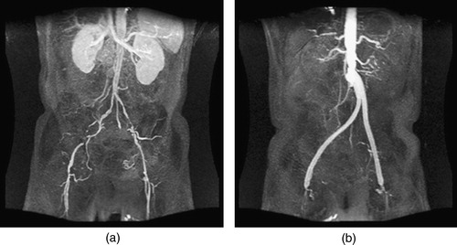
Figure 16. Views of the proximal anastomosis from the postoperative MRA dataset for the 55-year-old male. An isosurface of the postoperative MRA data set in the neighborhood of the proximal anastomosis is shown from two different angles. The distal native aorta occluded after surgery. [Color version available online]

Geometric modeling and operative planning

Prior to the patient's surgery, a preoperative model shown in Figure 17a was constructed. Owing to the significant vascular disease present, the arteries distal to the aortic bifurcation presented a geometric modeling challenge. On the patient's right side, for example, the right external iliac artery was occluded, and a collateral vessel branching off from the right common iliac artery had enlarged to feed the right femoral artery. The vessel was tortuous and small compared to the image resolution. Unlike the previous example, the profunda femoris arteries were highly visible in the scan (with several generations of branching), so they were included in the preoperative model.

Figure 17. Two bypass plans for 55-year-old male patient. (a) shows the preoperative model, (b) shows plan 1, and (c) shows plan 2. In (d), both plans are shown together to highlight differences between the two plans. [Color version available online]

Prior to the operation, the surgeon created two operative plans as shown in Figure 17. Plan 1 considered the option of using a 14 mm × 7 mm Dacron graft with an assumed uniform dilation of 14% (Figure 17b). Plan 2 considered the option of using a 16 mm × 8 mm Dacron graft with an assumed dilation of 22.5% for the bypass body and a 12.5% dilation of the bypass limbs. In addition, the location and path of the bypass are different in both surgical plans, as highlighted in Figure 17d. The variation in the location and path of the bypass is motivated both by the different size grafts and by the desire of the surgeon to test how differences in the procedure can impact the resulting flow. However, the location of the graft is limited by the anatomical structures of the body during actual placement.

A 16 mm × 8 mm Dacron graft was used in the actual surgery. The grafts are cut and trimmed specifically for each patient. When designing an anastomosis, the surgeon cuts the circular graft cross-section at an angle to create an elliptical cross-section to attach to the native vessel. This is done because it is believed that the resulting anastomosis leads to better hemodynamic conditions. The proximal anastomosis of the graft measured 27 mm × 16 mm prior to attachment to the native aorta. On the basis of the postoperative MRA data, the bypass body had a nominal diameter of 22 mm (37.5% dilation) and the bypass limbs were nominally 10 mm in diameter (25% dilation). For this case study, both surgical plans underestimated the dilation of the graft in vivo under physiological pressures.

Processing PCMRI data

In theory, processing the PCMRI data should resemble that for the previous example. In practice, however, there were acquisition problems that made processing the PCMRI data for this case study particularly difficult. Properly selecting encoding parameters can be a challenge, and for several of the slices of preoperatively acquired PCMRI data aliasing occurred (i.e., velocity wraparound as the velocity value is encoded in the phase angle). When acquiring PCMRI data, the operator sets a parameter (VENC) which is related to the maximum expected magnitude of velocity in a given slice location. Keeping the VENC low increases the accuracy of the velocity values obtained but risks aliasing. In this case study, however, higher-than-expected velocities were observed in the slices through the common iliac arteries preoperatively and aliasing occurred. Technical difficulties caused the postoperative MRA data and the PCMRI data to be acquired at different times. As the data were acquired on different days, the patient's physiology and position in the magnet could have changed between acquisitions, adding an additional source of error. Owing to the patient anatomy and boundary conditions used in the present study, only supra-celiac and infra-renal aorta volumetric flow rates were needed. From the preoperative scan, these were determined to be 1.8 liters/minute in the supra-celiac aorta and 0.7 liters/minute in the infra-renal aorta. On the basis of an estimate from a preoperative PCMRI slice plane at the aortic bifurcation, it appeared that 67.5% of the distal aortic flow was entering the right common iliac artery (∼470 ml/min) and 32.5% of the flow was entering the left common iliac artery (∼230 ml/min). Note that the right common iliac artery was providing flow to both the internal iliac artery and the femoral artery on the patient's right side.

Three-dimensional hemodynamic simulation

Isotropic tetrahedral meshes were generated for each plan shown in Figure 17. The mesh for plan 1 consisted of 1,781,661 elements (355,413 nodes) and the mesh for plan 2 consisted of 1,937,880 elements (382,393 nodes). These simulations were performed prior to the integration of resistance or impedance boundary conditions into the flow solver, so a combination of prescribed velocity and constant pressure outlets was used [3]. The three-component velocity data obtained experimentally from the preoperative PCMRI data were prescribed at the mesh inlet. Approximately 1.1 liters/minute of combined outflow was prescribed in the superior mesenteric, celiac trunk, and renal arteries. This effectively prescribed an infra-renal flow of 0.7 liters/minute. A simple distribution was assumed (22.7% to each renal artery, 27.3% to the celiac trunk and superior mesenteric artery) for the branch vessels between the supra-celiac and infra-renal image slices. The flow waveforms of the prescribed analytic boundary conditions were scaled versions of the inlet waveform.

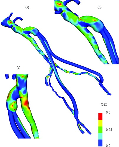
Blood flow simulations were performed assuming a blood viscosity of 0.04 poise and density of 1.06 g/cm³. A total of six cardiac cycles were simulated with 400 time steps per cardiac cycle. Simulations show flow in the distal native aorta between 170 and 200 ml/min postoperatively during resting conditions. Recall that the postoperative MRA data indicated that the distal native aorta occluded within 9 days of the surgery (Figure 15b). The results from the simulations presented here are not necessarily consistent with the clinically observed occlusion of the distal native aorta. In addition, as was the case in the previous example, clinically relevant quantities such as mean wall shear stress (Figure 18) and oscillatory shear index (Figure 19) were calculated.

Figure 18. Mean wall shear stress for plan 1. (a) the entire model; (b) an anterior view; and (c) a posterior view of the proximal anastomosis.

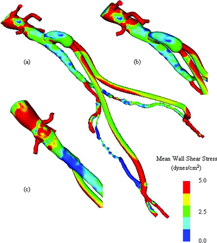
Figure 19. OSI for plan 1. (a) the entire model; (b) an anterior view; and (c) a posterior view of the proximal anastomosis.

Case summary

The significance of this case study was the demonstration of model construction and operative planning in a clinically relevant time frame. The preoperative model and PCMRI data were processed in less than 24 h after the data acquisition, and the surgeon was able to create two surgical plans prior to performing the actual surgery. Each plan required ∼1 h of the surgeon's time. The data for this case study presented additional processing challenges when compared with the previous example due to difficulties with the PCMRI acquisition. In addition, the closure of the native distal aorta was not expected. There are several possible explanations for the apparent inconsistency between the simulation results and the observed clinical outcome. One of the most likely is that when the surgeon clamped the native aorta during the operation, thrombus or plaque was dislodged and traveled downstream, impeding flow in the distal native aorta. It is currently unknown how frequently debris becomes dislodged due to surgical interventions.

Discussion

The methods and results presented in this work represent the most comprehensive investigation of using simulation-based techniques for aortoiliac occlusive treatment planning to date. The challenges in acquiring and processing MRA and PCMRI data for two patient data sets have been discussed in detail. A software system that enabled a vascular surgeon to preoperatively create geometric models representing alternative surgical procedures for a patient has been described. In addition, the system enabled the processing of PCMRI data for prescribing velocity boundary conditions needed for hemodynamic simulation. One- and three-dimensional simulation results have been presented and compared, and their respective trade-offs discussed.

The results of this work indicate several important potential research directions. First, improvements in image processing techniques to create preoperative models and process image data for flow and boundary information are vital. As discussed in the Results section, the resolution of the MRA data provides significant challenges when constructing models for diseased patients. Although the resolution of MRA imaging continues to improve, in recent years CTA resolution has significantly increased. It is now possible to acquire high-resolution full-body CT studies (1500 + slices). These data sets provide a practical challenge in that they typically contain over 1 GB of raw data, which may require special graphical hardware and algorithms just to interact with it. In addition, the high signal of bone in CTA provides segmentation challenges not found in processing MRA data.

The geometric challenges for simulation-based surgical planning of treatments for aortoiliac occlusive disease from CT data include creating accurate 3D geometric models in the abdomen and using the remaining anatomic information in the specification of the outflow boundary conditions applied to the 3D simulation domain. Challenges also remain in developing an intuitive, interactive environment for surgeons to create alternative surgical plans. Improvements in modeling synthetic graft dilation, balloon angioplasty, and stent deployment will likely be required to accurately predict the therapeutic benefit of various interventions.

It seems likely that the integration of one- and three-dimensional hemodynamic analysis into a common framework will be critical in developing clinically applicable protocols and software tools, given their corresponding trade-offs for accuracy and computational expense. The results discussed in this paper motivate investigation of additional improvements in one-dimensional modeling, including additional complex downstream boundary conditions and improved minor loss terms for special conditions such as flow in a stenosis, junction losses, and flow in aneurysms. In three dimensions, research into relaxing the assumption of rigid vessel walls and integration of impedance boundary conditions is underway. Modeling the viscoelastic properties of the vessel wall and the non-Newtonian behavior of blood may also improve the accuracy of the simulations.

Finally, additional experimental validation studies and clinical trials are essential to improve the numerical models and quantify the accuracy of these predictive methods. The patients selected for this study were chosen because they were scheduled to undergo direct vascular reconstructions. The differences between direct revascularization and endovascular repair may be less dramatic for patients with less extensive vascular disease. Open surgical and endovascular procedures have significantly different risks of complications, cost, and therapeutic benefit to the patient. Some vascular surgeons today argue that the standard of care should be to resort to open surgical procedures only if minimally invasive procedures fail. This philosophy can subject patients to unnecessary procedures which yield little clinical benefit. In addition, the mounting cost of health care worldwide continues to be an important socio-political issue. Providing further insight into the benefit of alternate interventions for individual patients may assist public planners [62] in creating health-care reimbursement policy.

Acknowledgments

This material is based on work supported by the National Science Foundation under Grant no. 0205741. The authors gratefully acknowledge Dr Mette Olufsen for the use of her methods to compute input impedance of vascular trees, Dr Farzin Shakib for his linear algebra package (http://www.acusim.com), and Professor Kenneth Jansen at Rensselaer for the use of his finite-element flow solver. Finally, the authors gratefully acknowledge the assistance of Dr Mary Draney for acquiring the subject-specific MRI data and Irene Vignon for her assistance with resistance and impedance boundary conditions.

References

- Rutherford R B. Vascular surgical procedures. R B Rutherford. WB Saunders Company, Philadelphia, PA 2000
- Taylor C A, Draney M T, Ku J P, Parker D, Steele B N, Wang K, Zarins C K. Predictive medicine: computational techniques in therapeutic decision-making. Comput Aided Surg 1999; 4: 231–247
- Wilson N M. Geometric algorithms and software architecture for computational prototyping: applications in vascular surgery and MEMS. Department of Mechanical Engineering, Stanford University, Stanford, CAUSA December, 2002, PhD Dissertation
- Wilson N M, Wang K, Dutton R W, Taylor C A (2001) A software framework for creating patient specific geometric models from medical imaging data for simulation based medical planning of vascular surgery. Proceedings of the 4th International conference on Medical Image Computing and Computer-Assisted Intervention (MICCAI 2001), UtrechtThe Netherlands, October, 2001, W Niessen, M Viergever. Springer;, Berlin, 449–456, Lecture Notes in Computer Science Vol. 2208
- Taylor C A. A computational framework for investigating hemodynamic factors in vascular adaptation and disease. Department of Mechanical Engineering, Stanford University, Stanford, CAUSA August, 1996, PhD Dissertation
- Wilson N M, Arko F R, Taylor C A (2004) Patient-specific operative planning for aortofemoral reconstruction procedures. Proceedings of the 7th International Conference on Medical Image Computing and Computer-Assisted Intervention (MICCAI 2004), St. MaloFrance, October, 2004, C Barillot, D R Haynor, P Hellier. Springer;, Berlin, 422–429, Lecture Notes in Computer Science Vol. 3217
- Wilson N M, Arko F R, Zarins C K, Olcott C, Taylor C A. Preoperative computational modeling of aortofemoral reconstructions to predict postoperative hemodynamic results. Proceedings of the 32nd Annual Symposium on Vascular Surgery, Rancho Mirage, CA, 10–13 March, 2004, 110
- Wilson N M, Arko F R, Taylor C A. An integrated software system for preoperatively evaluating aortofemoral reconstruction procedures. Proceedings of the American Society of Mechanical Engineers Summer Bioengineering Conference, Miami, FL, 25–29 June, 2003, 899–900
- Draney M T, Alley M T, Tang B T, Wilson N M, Herfkens R J, Taylor C A. Importance of 3D nonlinear gradient corrections for quantitative analysis of 3D MR angiographic data. Proceedings of International Society for Magnetic Resonance in Medicine Tenth Scientific Meeting & Exhibition (ISMRM 2002), Honolulu, Hawaii, 18–24 May, 2002
- Ku J P, Draney M T, Arko F R, Lee W A, Chan F P, Pelc N J, Zarins C K, Taylor C A. In vivo validation of numerical predication of blood flow in arterial bypass grafts. Ann Biomed Eng 2002; 30: 743–752
- Steele B N, Wan J, Ku J P, Hughes T J.R, Taylor C A. In vivo validation of a one-dimensional finite element method for simulation-based medical planning for cardiovascular bypass surgery. IEEE Trans Biomed Eng 2003; 50: 649–656
- Ku J P, Elkins C J, Taylor C A. Comparison of CFD and MRI flow and velocities in an in vitro larger artery bypass graft model. Ann Biomed Eng 2005; 33(3)257–269
- Paik D S, Beaulieu C F, Jeffrey R B, Rubin G D, Napel S. Automated flight path planning for virtual endoscopy. Med Phys 1998; 25: 629–637
- Schroeder W, Martin K, Lorensen W. The Visualization Toolkit. Prentice-Hall;, New Jersey 1998
- Wang K. Level set methods for computational prototyping with application to hemodynamic modeling. Department of Electrical Engineering, Stanford University, Stanford, CAUSA August, 2001, PhD Dissertation
- Osher S, Sethian J A. Fronts propagating with curvature-dependent speed: algorithms based on Hamilton–Jacobi formulations. J Comput Phys 1988; 79: 12–49
- Malladi R, Kimmel R, Adalsteinsson D, Sapiro G, Caselles V, Sethian J A. A geometric approach to segmentation and analysis of 3D medical images. Proceedings of the Workshop on Mathematical Methods in Biomedical Image Analysis, San Francisco, CA, June, 1996, 244–252
- Sethian J A. Level set methods and fast marching methods. Cambrige University Press;, Cambridge 1999
- Parasolid reference manual, EDS, Inc., Plano, TX, USA
- Davidovic L B, Lotina S I, Kostic D M, Cinara I I, Cvetkovic S D, Stojanovic P L, Velimirovic L B, Markovic D M, Pejkic S L, Pavlovic G. Dacron and polytetrafluoroethylene aortobifemoral grafts. Srp Arh Celok Lek 1997; 125(3–4)75–83
- Devine C, McCollum C. Heparin-bonded dacron or polytetrafluoroethylene for femoralpopliteal bypass grafting: a multicenter trial. J Vasc Surg 2001; 33(3)533–539
- Zakhariev T, Grozdinski L, Stankev M, Chirkov A. A comparative assessment of the results of end-to-end and end-to-side anastomoses in arterial reconstructions of the aortoiliac segment. Khirurgiia (Sofiia) 1995; 48(1)37–42
- den Hoed P T, Veen H F. The late complications of aortoilio-femoral Dacron prostheses: dilatation and anastomotic aneurysm formation. Eur J Vasc Surg 1992; 6(3)282–287
- van der Akker P J, Brand R, van Schilfgaarde R, van Bockel J H, Terpstra J L. False aneurysms after prosthetic reconstructions for aortoiliac obstructive disease. Ann Surg 1989; 210(5)658–666
- Harris P, How T. Haemodynamics of cuffed arterial anastomoses. Int J Vasc Med 1999; 9(1)20–26
- Sieswerda C, Skotnicki S H, Barentsz J O, Heystraten F M. Anastomotic aneurysms—an underdiagnosed complication after aortoiliac reconstructions. Eur J Vasc Surg 1989; 3(3)233–238
- Swartbol P, Albrechtsson U, Parsson H, Norgren L. Dialation of aortobifemoral knitted Dacron grafts after a mean implantation of 5 years. Int Angiol 1996; 15(3)236–239
- Florez-Valencia L, Montagnat J, Orkisz M (2002) 3D graphical models for vascular-stent pose simulation. Proceedings of International Conference on Computer Vision and Graphics (ICCVG), Zakopane, Poland, September, 2002, 25–29
- Isokangas J M, Hietala R, Perala J, Tervonen O. Accuracy of computer-aided measurements in endovascular stent-graft planning. Invest Radiol 2003; 38(3)164–170
- Dumoulin C, Cochelin B. Mechanical behaviour modelling of balloon-expandable stents. J Biomech 2000; 33: 1461–1470
- Coenegrachts K, Rigauts H, Letter J D. Prediction of aortoiliac stent graft length: comparison of a semiautomated computed tomography angiography method and calibrated aortography. J Comp Assist Tomogr 2003; 22(2)284–288
- Auricchio F, Loreto M D, Sacco E. Finite-element analysis of a stenotic artery revascularization through a stent insertion. Comp Methods Biomech Biomed Eng 2001; 4: 249–263
- Holzapfel G A, Schulze-Bauer CAJ, Stadler M. Mechanics of angioplasty: wall, balloon and stent. Proceedings in Mechanics in Biology, J Casey, G Bao. New York 2000; AMD-Vol. 242, BED-Vol. 46: 141–156
- Pelc N J, Herkens R J, Shimakawa A, Enzmann D R. Phase contrast cine magnetic resonance imaging. Magn Reson Quart 1991; 7(4)229–254
- Pelc N J, Sommer F G, Li KCP, Brosnan T J, Herfkens R J, Enzmann D R. Quantitative magnetic resonance flow imaging. Magn Reson Quart 1994; 10(3)125–147
- Figueroa C A, Jansen K C, Hughes TJR, Taylor C A. A coupled momentum method to model blood flow in deformable arteries. Proceedings Sixth World Congress on Computational Mechanics, BeijingChina, 5–10 September, 2004, Paper n. o. 635 on CDROM
- Womersley J R. Oscillatory motion of a viscous fluid in a thin-walled elastic tube—I: the linear approximation for long waves. Phil Mag 1955; 7: 199–221
- Wan J, Steele B, Spicer S A, Strohband S, Feijoo G R, Hughes TJR, Taylor C A. A one-dimensional finite element method for simulation-based medical planning for cardiovascular disease. Comp Methods Biomech Biomed Eng 2002; 5(3)195–206
- Steele B N. A simulation-based medical planning system for occlusive cardiovascular disease using one dimensional analysis techniques. Department of Mechanical Engineering, Stanford University, Stanford, CAUSA August, 2003, PhD dissertation
- Vignon I E, Taylor C A. Outflow boundary conditions for one-dimensional finite element modeling of blood flow and pressure waves in arteries. Wave Motion 2004; 39: 361–374
- Steele B N, Taylor C A. Simulation of blood flow in the abdominal aorta at rest and during exercise using a 1-D finite element method with impedance boundary conditions derived from a fractal tree. In:. Proceedings of ASME Summer Bioengineering Meeting, Key Biscayne, FL, June, 2003, 813–814
- Müller J, Nagrath S, Li X, Jansen K E, Shephard M S. Efficient computational methods for the investigation of cardiovascular disease. Proceedings of the US National Congress on Computational Mechanics (USNCCM7), Albuquerque, NM, July, 2003
- Taylor C A, Hughes TJR, Zarins C K. Finite element modeling of blood flow in arteries. Comp Methods Appl Mech Eng 1998; 158: 155–196
- Taylor C A, Hughes TJR, Zarins C K. Finite element modeling of three-dimensional pulsatile flow in the abdominal aorta: relevance to atherosclerosis. Ann Biomed Eng 1998; 26: 975–987
- Taylor C A, Hughes TJR, Zarins C K. Effect of exercise on hemodynamic conditions in the abdominal aorta. J Vasc Surg 1999; 29(6)1077–1089
- Vignon I E, Figueroa C A, Jansen K E, Taylor C A. Outflow boundary conditions for three-dimensional finite element modeling of blood flow and pressure in arteries. Comp Meth Appl Mech Eng, in press
- Taylor C A, Hughes TJR. A multiscale finite element method for blood flow in deformable vessels. Proceedings of the 1998 World Congress of Biomechanics. SapporoJapan 1998
- Shim E B, Kamm R D, Heldt T, Mark R G. Numerical analysis of blood flow through a stenosed artery using a coupled multiscale simulation method. Comp Cardiol 2000; 27: 219–222
- Laganà K, Dubini G, Migliavacca F, Pietrabissa R, Pennati G, Veneziani A, Quarteroni A. Multiscale modelling as a tool to prescribe realistic boundary conditions for the study of surgical procedures. Biorheology 2002; 39(3–4)359–364
- Formaggia L, Gerbeau J F, Nobile F, Quartoni A. Numerical treatment of defective boundary conditions for the Navier–Stokes equations. SIAM J Numer Anal 2002; 40(1)376–401
- Formaggia L, Gerbeau J F, Nobile F, Quartoni A. On the coupling of 3D and 1D Navier–Stokes equations for flow problems in compliant vessels. Comp Meth Appl Mech Eng 2001; 191: 561–582
- Franca L P, Frey S L. Stabilized finite element methods i. i. The incompressible Navier–Stokes equations. Comp Methods Appl Mech Eng 1992; 99(2–3)209–233
- Jansen K E, Whiting C H, Hulbert G M. Generalized-α method for integrating the filtered Navier–Stokes equations with a stabilized finite element method. Comp Methods Appl Mech Eng 2000; 190(3–4)305–319
- Whiting C H, Jansen K E. A stabilized finite element method for the incompressible Navier–Stokes equations using a hierarchical basis. Int J Numer Methods Fluids 2001; 35: 93–116
- Brooks A N, Hughes TJR. Streamline upwind Petrov–Galerkin formulation for convection dominated flows with particular emphasis on the incompressible Navier–Stokes equations. Comp Methods Appl Mech Eng 1981; 32: 199–259
- Karypis G, Kumar V. Multilevel algorithms for multi-constraint graph partitioning. University of Minnesota. Department of Computer Science/Army HPC Research Center, Minneapolis, Technical Report no. 98—019
- Cheng C P, Parker D, Taylor C A. Quantification of wall shear stress in large blood vessels using Lagrangian interpolation functions with cine PC-MRI. Ann Biomed Eng 2002; 30(8)1020–1032
- Taylor C A, Cheng C P, Espinosa L A, Tang B T, Parker D, Herfkens R J. In vivo quantification of blood flow and wall shear stress in the human abdominal aorta during lower limb exercise. Ann Biomed Eng 2002; 30(3)402–408
- Ganong W FM. Review of medical physiology. Englewood Cliffs: Appleton & Lange 1995
- Cheng C P, Herfkens R J, Taylor C A. Comparison of abdominal aortic hemodynamics between men and women at rest and during lower limb exercise. J Vasc Surg 2002; 37(1)118–123
- Seeley B D, Young D F. Effect of geometry on pressure losses across models of arterial stenoses. J Biomech 1976; 9(7)439–448
- Post P N, Kievit J, van Bockel J H. Optimal follow-up strategies after aortoiliac prosthetic reconstruction: a decision analysis and cost-effectiveness analysis. Eur J Vasc Endovasc Surg 2004; 28(3)287–295