Blending Bayesian and Classical Tools to Define Optimal Sample-Size-Dependent Significance Levels

ABSTRACT

This article argues that researchers do not need to completely abandon the p-value, the best-known significance index, but should instead stop using significance levels that do not depend on sample sizes. A testing procedure is developed using a mixture of frequentist and Bayesian tools, with a significance level that is a function of sample size, obtained from a generalized form of the Neyman–Pearson Lemma that minimizes a linear combination of α, the probability of rejecting a true null hypothesis, and β, the probability of failing to reject a false null, instead of fixing α and minimizing β. The resulting hypothesis tests do not violate the Likelihood Principle and do not require any constraints on the dimensionalities of the sample space and parameter space. The procedure includes an ordering of the entire sample space and uses predictive probability (density) functions, allowing for testing of both simple and compound hypotheses. Accessible examples are presented to highlight specific characteristics of the new tests.

KEYWORDS:

• Hardy–Weinberg equilibrium
• Neyman–Pearson lemma
• Predictive distribution
• Significance test

1 Introduction

It has become clear that the tests performed by comparing a p-value to 0.05 are not adequate for science in the 21st Century. Classical p-values have multiple problems that can make the results of hypothesis tests difficult to understand, multiple kinds of “p-hacking” can be used to try to get a p-value below the “magic” number of $0.05,$ and as many researchers have discovered, tests using standard p-values just aren’t useful when the sample size gets large, because they end up rejecting any hypothesis. Jeffreys’s tests using Bayes factors with fixed cutoffs also tend to have problems with large samples. However, hypothesis testing is a useful tool and is now a more-than-familiar way of thinking about how to do experiments and a very broadly used way of understanding and reporting experimental results. What is a researcher to do?

The present article introduces one solution for researchers who recognize that the hypothesis tests of the 20th Century are inadequate, but don’t want to have to change the way they think about experiments and the ways they interpret and report experimental results. Section 2 delves into some of the problems that arise with the most widely used hypothesis tests and why those problems occur. Section 3 presents a new kind of hypothesis test that avoids the problems described, but doesn’t “throw out the baby with the bath water,” retaining the useful concept of statistical significance and the same operational procedures as currently used tests, whether frequentist (Neyman–Pearson p-value tests) or Bayesian (Jeffreys’s Bayes-factor tests). Section 4 presents examples of the new tests being used, to highlight some of the advantages of the new tests and show researchers operational details of how the new tests can be used. Final considerations are given in Section 5. The article is written for researchers who are interested in a more modern tool for hypothesis testing, but who are not necessarily statisticians. It therefore does not go into deep theoretical detail, focusing instead on issues of more direct relevance to would-be users of the new tests. However, references are provided for those interested in the details of the theory behind the tests.

2 Context and Motivation: What’s Wrong With the Tests People Have Been Using for so Many Years?

The subject of hypothesis testing and some of the problems that arise has been the subject of vigorous debate for several decades. Because frequentist tests using p-values are the most widely used, the use of p-values has been the subject of the most and harshest criticism. The journal Basic and Applied Social Psychology even went so far as to prohibit the use of p-values in articles—see Trafimow and Marks (2015). The controversy over the use of p-values has been so great that the American Statistical Association issued an official statement on p-values: Wasserstein and Lazar (2016).

It is worth saying that hypothesis tests based on p-values are not the only tools subject to valid criticism. Hypothesis testing in general has been criticized, for example, in Cohen (1994), Levine et al. (2008), and Tukey (1969), and some of the alternative methods of hypothesis testing, such as the Bayes-factor hypothesis tests created by Jeffreys, have been the subject of specific criticisms like those of Gelman and Rubin (1995) and Weakliem (1999). Further, hypothesis tests are not the only statistical tools that can be criticized. Every statistical tool relies on a model of some kind, and ultimately seeks to do something that can’t be done in an exact and perfect way: make inferences based on limited quantities of data. Even when there are many, many data available, the sample is always finite, and so the inference must be imperfect. As a result, there are valid criticisms of every statistical tool. Tests based on p-values get special attention because of the fact that they are so widely used, and their misuse has contributed greatly to the “reproducibility crisis” in science and medicine.

The way p-values are used in statistical tests is based on the work of Fisher and of Neyman and Pearson in the 1930s. Fisher produced “significance tests” in which a “null hypothesis” about a parameter in a statistical distribution is tested without any consideration of what the alternative or alternatives are. Neyman and Pearson created “hypothesis tests,” in which a null hypothesis is tested against a specific alternative or alternatives. In both cases, the null hypothesis is usually something like “there is no effect.”¹ When the null is rejected, the inference is that there is some interesting effect to be reported. In both cases, the null is rejected based on the comparison of a p-value to a “significance level.” A p-value has multiple possible definitions. It is not always defined as a probability (see, for example, Schervish (2012)), but its calculation is always a probability calculation. Given an experimental result $x_0,$ a p-value is calculated as the probability, if the null hypothesis were true, of an observation x that supports the null hypothesis as much or less than the actual experimental result $x_0.$ When the p-value is sufficiently small, the researcher decides that the actual observation x₀ is sufficiently unlikely under the null hypothesis that he or she can conclude that the null is false.

How small is “sufficiently small”? This is where the concept of “statistical significance” comes into the story. The p-value is generally compared to some small number that ends up being the probability of incorrectly rejecting a null hypothesis that is true. In his original work on significance testing, Fisher mentioned a one-in-twenty chance ($5\%,$ or 0.05) of rejecting a correct null as a convenient cutoff for declaring a statistically significant result, but did not intend for this number to be used universally. He states in his 1956 article “Statistical Methods and Scientific Inference” that the significance level should be set according to the circumstances. In the seminal work on statistical hypothesis testing, Neyman and Pearson (1933), an attempt is made to explicitly control errors in finding the best kind of test to choose between a null hypothesis and one or more specific alternative hypotheses. Two kinds of possible errors are considered: rejecting a true null hypothesis, called “errors of the first kind” (here called“errors of type I” or “type-I errors”) and accepting a false null hypothesis, an “error of the second type” (here, “type-II error”). Neyman and Pearson write “The use of these statistical tools in any given case, in determining just how the balance should be struck, must be left to the investigator,” where “the balance” refers to the balance between the probabilities of the two types of error. Ironically enough, the very mathematical approach adopted by Neyman and Pearson makes it close to impossible for a researcher to determine “just how the balance should be struck.” Neyman and Pearson fix the probability of a type-I error, which is denoted here and in many statistics texts as $\alpha ,$ and then prove that the test that minimizes the probability of a type-II error, here and elsewhere denoted as $\beta ,$² is a test based on comparing the ratio of the likelihoods³ of the competing hypotheses to some cutoff value, with the cutoff chosen so that the probability of incorrectly rejecting a correct null hypothesis is $\alpha .$ As shown in Pericchi and Pereira (2016), adopting this approach can lead to imbalances so great that the probabilities of the two types of error can vary by orders of magnitude.

In addition to the imbalance between the error probabilities of the two types described above, fixing α can lead to an even more serious problem. Because p-values tend to decrease with increasing sample size, the easiest and most common form of “p-hacking” is to keep taking data until the p-value falls below 0.05 or whatever other level of significance is chosen and fixed. No matter what level is chosen, a large-enough sample will almost inevitably lead to rejection of any null hypothesis. In the words of Berger and Delampady (1987), “In real life, the null hypothesis will always be rejected if enough data are taken because there will be inevitably uncontrolled sources of bias.” According to Pericchi and Pereira (2016), more information paradoxically ends up being “a bad thing” for Neyman–Pearson hypothesis testing (and Fisherian signficance testing). Fixing a lower value for declaring a statistically significant result, say, 0.005 instead of $0.05,$ as suggested recently by a group of 72 researchers, many of them quite prominent, and some of them highly respected statisticians (Benjamin et al. (2018)), will only postpone the problem to larger sample sizes. This is folly even at the dawn of the era of “Big Data,” and not a good solution in general. More data will still be “a bad thing” for tests with a cutoff that is lower, but still fixed, in direct conflict with the common-sense idea that a result based on a larger sample should be more believable.

A definition of the p-value for a null hypothesis H and observation x₀ commonly used in statistics textbooks is represented in Pereira and Wechsler (1993) as follows⁴:

Definition 1

(PW2.2). The p-value is the probability, under H, of the event composed by all sample points that are at least as extreme as x₀ is.

“[S]ample points” here refers to possible experimental observations. Note that this definition does not in any way take into account the alternative hypothesis $\mathbf{A}.$ One problem with this definition is that in some cases, a p-value defined this way can’t even be calculated. For example, when the range of possible observations (“sample space”) consists of separate intervals, or when it is multidimensional, it can be unclear what “extreme” means. Throughout this article, “p-value,” with a lower-case “p,” is used to refer to a quantity calculated using Definition 1. A contrasting definition of a quantity analogous to the small-p p-value was presented in Pereira and Wechsler (1993) and is reproduced in the next section, along with an explanation of its advantages over traditional p-values.

Another problem with commonly used hypothesis tests is that the results can be hard to interpret, and their correct interpretation depends on the intent of the experimenter. An issue that has been the subject of vigorous debate among statisticians for decades is the Likelihood Principle (LP). While it still has the status of a principle that one either accepts or does not⁵, and there are greatly respected statisticians who do not accept the LP, it is still true that LP-compliant tests have intuitive appeal and can be easier to interpret. For example, Cornfield (1966), Lindley and Phillips (1976), and Berger and Wolpert (1988) show that while frequentist tests that are not LP-compliant can give conflicting results for the same data, depending on what “stopping rule” is chosen for an experiment, the results of LP-compliant tests do not depend on the stopping rule and permit a single, unique inference based on the data without needing to know the intent of the experimenters. This brings the added advantage of allowing the collected data to be used while permitting researchers to stop an experiment early. Ethics can demand an early end to an experiment, for example, in the case of a medical study in which it becomes very clear that the patients receiving a new treatment are recovering, while those in the control group are not, or when patients receiving a new treatment are suffering serious side effects. Non-LP-compliant tests would require the researchers either to carry out the experiments to their pre-planned end, possibly in conflict with medical ethics, or to throw away all the collected data upon being forced by ethical concerns to stop the experiments earlier than planned.

There are Bayesian alternatives to frequentist hypothesis tests, the tests based on Bayes factors created by Jeffreys in the 1930s (see Jeffreys (1935, 1939)) and reviewed 60 years later in Kass and Raftery (1995). They are not as widely used as frequentist tests, but they have gained some acceptance in certain areas of research and are sometimes held up as a better alternative. As noted earlier, no tool is perfect, and Bayes-factor tests have also been criticized by both Bayesian and frequentist statisticians. For the purposes of this article, it is worth noting that Bayes factors, once calculated, are also compared to fixed cutoffs in Jeffreys’s tests. The calculation of Bayes factors is described in the next section. For now, it is enough to know that the Bayes factor ${\text{BF}}_{\mathbf{HA}}$ is a measure of the evidence favoring H over $\mathbf{A}.$ Jeffreys proposed an initial table of evidence grades against a null hypothesis $\mathbf{H},$ with cutoffs at half-integer powers of 10, and Kass and Raftery updated the table by reducing the number of grades of evidence, noting that the Bayes factor measuring evidence against a null hypothesis H in favor of an alternative $\mathbf{A}, {\text{BF}}_{\mathbf{AH}}$, is $1/{\text{BF}}_{\mathbf{HA}}$, and compiling a table of cutoff values of ${\text{BF}}_{\mathbf{AH}}$. No justification is given for the cutoffs, other than Kass and Raftery stating “From our experience, these categories seem to furnish appropriate guidelines.” Jeffreys’s Bayes-factor tests do not take experimental error into account, and the cutoffs, whether those proposed by Jeffreys or those proposed by Kass and Raftery, do not take sample size into account. As with frequentist hypothesis tests with fixed cutoffs, inconvenient behavior with large samples is to be expected. This manifests itself in multiple ways, including a tendency of Bayes factors to favor null hypotheses strongly for large samples, especially in cases of small effect sizes.

3 Solving Some of the Problems in Hypothesis Testing

Most readers of this article already knew before starting to read it that there are some problems with the kinds of hypothesis testing done in many fields of research. In the previous section, some of those problems have been described in a bit more detail than a news article can usually dedicate to the subject. So now what? What can a researcher do? In this section, one solution is presented, and some of its advantages over currently used hypothesis tests are described. The approach uses both frequentist and Bayesian methods and results in hypothesis tests that are operationally very similar to the commonly used tests that compare a p-value to a significance level $\alpha .$

The authors of this article take the position taken over 60 years ago by both a Bayesian statistician, Lindley (1957), and a frequentist statistician, Bartlett (1957): a major part of the problems with p-value-based tests is in fixing a significance level that does not depend on the sample size. That is, the problem is not as much in the use of p-values themselves as in comparing p-values to fixed signficance levels. The solution to this issue is surprisingly simple and is rooted in the presentation of Neyman and Pearson’s lemma in DeGroot’s widely used textbook (DeGroot 1986), perhaps the greatest bridge between the frequentist and Bayesian “schools” of statistics. Instead of starting with a fixed α and determining the tests that minimize β as Neyman and Pearson did, DeGroot presented a generalized form of the Neyman–Pearson Lemma in which a linear combination of α and β is minimized. When α is then fixed, the result is the same as the one presented by Neyman and Pearson in 1933. In its full generality, the version presented by DeGroot has a major advantage: by minimizing a linear combination of α and $\beta ,$ it allows the probabilities of both types of error to vary, avoiding the kind of drastic imbalance between the probabilities of the two types of errors described in Pericchi and Pereira (2016), because instead of α being fixed and β tending to decrease with increasing sample size, both error probabilities depend on the sample size. By controlling the ratio of the coefficients of α and β in the linear combination that is minimized, a researcher can actually determine “just how the balance should be struck,” realizing the vision of Neyman and Pearson in a way Neyman-Pearson tests simply cannot. Cornfield (1966) suggested optimizing tests by minimizing a linear combination of α and β.

How should the coefficients a and b in the linear combination $a\alpha +b\beta$ be chosen? The coefficients a and b represent the relative seriousness of errors of the two types or, equivalently, relative prior preferences for the competing hypotheses. If, for example, $a>b,$ that means type-I errors are considered more serious than type-II errors. That means incorrectly rejecting H in favor of A is considered more serious than incorrectly rejecting A in favor of $\mathbf{H},$ which indicates a prior preference for $\mathbf{H}.$ Here is a concrete example: imagine a state in which there have been more cases of meningitis than usual, and where the governor is very budget-conscious. Take H to be the hypothesis that there is not a meningitis epidemic in the state, and A to be the competing hypothesis that there is an epidemic. The governor may consider the unnecessary spending from an incorrect rejection of H to be more serious than the consequences of not declaring an epidemic, or equivalently, favor hypothesis H over $\mathbf{A},$ and so would set $a>b.$ Decision theory allows for the underlying assumptions to be made even more explicit by going more deeply into the meaning of a and b. The details can be found in the section on “Bayes test procedures” in DeGroot (1986), but the important point here is that if the losses due to incorrect rejection of each hypothesis can be quantified, and the prior probability that H is true can be estimated, then a and b can be calculated from those numbers. It is worth mentioning that the absolute scale of a and b, and therefore the absolute scale of the losses from the two possible types of errors, do not matter; only the ratio of a and b affects the actual decision whether to reject a hypothesis.

The Neyman–Pearson Lemma and the extended version of it presented by DeGroot are proved for simple-vs.-simple hypotheses, that is, for comparing specific values of a parameter. For example, for a normal (Gaussian) distribution with mean θ and variance $1, \mathcal{N}(\theta ,1),$ one might compare the hypotheses $\mathbf{H}:\theta =0$ and $\mathbf{A}:\theta =0.7.$ For a given observation x, the ratio of likelihoods $\ell (\theta =0|x)/\ell (\theta =0.7|x)$ would be compared to a cutoff chosen so that the probability, under hypothesis $\mathbf{H},$ that is, if x obeyed a $\mathcal{N}(0,1)$ distribution, of an observation falling in the rejection region would be some fixed value $\alpha ,$ like the commonly used 0.05 or the recently suggested 0.005. For certain types of distributions and certain types of hypotheses (see DeGroot (1986) or other statistics textbooks for details), the Neyman–Pearson Lemma can be extended to find the best tests for composite hypotheses, that is, hypotheses involving multiple values or continuous ranges of values of the parameter of interest. A Bayesian approach to extending beyond optimal simple-vs.-simple hypothesis tests offers a simple and obvious way to extend to tests where one or both of the hypotheses can be composite hypotheses, and where either or both hypotheses may be very complex.

As usual, consider a random vector x representing experimental results, with a probability (density) function⁶ $f(x|\theta )$ having a parameter vector $\theta ,$ with x and θ elements of real sample space $\mathfrak{X}$ and parameter space $\Theta ,$ respectively, each space having some positive integer dimensionality. The competing hypotheses H and A must partition the parameter space, that is, divide it into nonoverlapping pieces ${\Theta }_{\mathbf{H}}$ and ${\Theta }_{\mathbf{A}}$ such that the hypotheses can be expressed as(1) $$\mathbf{H}: \theta \in {\Theta }_{\mathbf{H}} \text{and} \mathbf{A}: \theta \in {\Theta }_{\mathbf{A}}.$$(1)

As long as the two pieces make up the entire space ($\Theta ={\Theta }_{\mathbf{H}}\cup {\Theta }_{\mathbf{A}}$) and do not overlap (${\Theta }_{\mathbf{H}}\cap {\Theta }_{\mathbf{A}}=\varnothing$), the hypotheses can be of any dimensionality and arbitrarily complex.

Define the binary parametric function $\lambda (\theta )$ as follows:(2) $$\lambda (\theta )=\{\begin{array}{cc}0\hfill & \theta \in {\Theta }_{\mathbf{H}}\hfill \\ 1\hfill & \theta \in {\Theta }_{\mathbf{A}}.\hfill \end{array}$$(2)

Because λ is a function of $\theta ,$ one can write(3) $$f\left(x\right|\theta )=f(x|\theta ,\lambda ).$$(3)

Now treat the original parameter θ as a “nuisance parameter” and remove it the Bayesian way: by taking averages of $f(x|\theta ,\lambda ),$ weighted by a prior $g(\theta ),$ over the two pieces of the parameter space ${\Theta }_{\mathbf{H}}$ and ${\Theta }_{\mathbf{A}}.$ The result is two predictive probability (density) functions(4) $$\begin{array}{cc}{f}_{\mathbf{H}}\left(x\right)\hfill & =f\left(x\right|\lambda =0) \text{and}\hfill \\ f_{\mathbf{A}}\left(x\right)\hfill & =f\left(x\right|\lambda =1).\hfill \end{array}$$(4)

Using the approach based on the generalized form of the Neyman–Pearson Lemma presented by DeGroot and previously used by Cornfield, as described earlier in this section, but now with the likelihoods averaged over ${\Theta }_{\mathbf{H}}$ and ${\Theta }_{\mathbf{A}}$ to produce $f_{\mathbf{H}}$ and $f_{\mathbf{A}},$ one obtains averaged error probabilities α and β that are optimal in the sense of the generalized Neyman–Pearson Lemma, and the optimal averaged α can be used as a significance level that depends strongly on the sample size.

As stated in the previous section, one problem with hypothesis tests comes from the use of definitions like Definition 1 to calculate p-values. A second definition that takes into account the alternative hypothesis $\mathbf{A},$ unlike Definition 1, is presented in Pereira and Wechsler (1993). As in the previous definition, x₀ represents the observation and H is the null hypothesis.

Definition 2

(PW2.1). The P-value is the probability, under $\mathbf{H},$ of the event composed by all sample points that favor A (against H) at least as much as x₀ does.

Note that the quantity defined here is a capital-P “P-value,” to distinguish it from the small-p “p-values” defined by Definition 1. The P-value has the advantage that, unlike a small-p p-value, it can be calculated for arbitrarily complex hypotheses that lead to arbitrarily complex rejection regions (regions where $p<\alpha ,$ where the null hypothesis would be rejected if the experimental observations were to occur there). However, to do so, it requires an ordering of the space of possible observations, the sample space, according to how much each possible observation favors one of the hypotheses over the other. The new approach, like Montoya-Delgado et al. (2001), uses the Bayes factor(5) $${\text{BF}}_{\mathbf{HA}}\left(x\right)=\frac{f_{\mathbf{H}}\left(x\right)}{f_{\mathbf{A}}\left(x\right)}$$(5) to order the sample space according to how much each point x favors H over $\mathbf{A}.$ Then, if the experiment yields a result $x_0,$ the P-value is calculated as the probability, given probability (density) function $f_{\mathbf{H}}(x),$ of a point in the sample space favoring A as much as or more than x₀ does. That is, it is the sum or integral of the probability (density) function $f_{\mathbf{H}}(x)$ over the part of the sample space where the Bayes factor ${\text{BF}}_{\mathbf{HA}}(x)$ is less than or equal to the Bayes factor calculated at $x_0.$ Calling that part of the sample space $\Psi ,$ it is defined as(6) $$\Psi =\left\{x\in \mathfrak{X}:{\text{BF}}_{\mathbf{HA}}\left(x\right)\le {\text{BF}}_{\mathbf{HA}}\left(x_0\right)\right\},$$(6) and the P-value is(7) $$P=\{\begin{array}{cc}\sum _{\Psi }{f}_{\mathbf{H}}\left(x\right),\hfill & \mathfrak{X} \text{discrete}\hfill \\ \underset{\Psi }{\int }{f}_{\mathbf{H}}\left(x\right)\mathit{dx},\hfill & \mathfrak{X} \text{continuous}.\hfill \end{array}$$(7)

There is a one-to-one correspondence between the P-value used in this approach and the Bayes factors used to calculate them, so once a cutoff for P—a significance level α—is determined, a corresponding cutoff for Bayes factors at the same significance level can be determined. As a result, researchers who are more comfortable with Bayes-factor tests can continue to use them, but with a cutoff determined by this method, which takes experimental error into account and depends on the sample size, rather than with arbitrarily defined cutoffs like those of Jeffreys (1935) or Kass and Raftery (1995).

4 Examples

Here some specific examples of applications of the new tests are presented. An important point emphasized throughout is the way the significance level varies with sample size.

4.1 Bernoulli (“Yes–No”) Examples

Though they are the simplest models, Bernoulli models, which are used for experiments with a “yes–no” result, like “heads-or-tails” coin flips, are very important. This is because many medical studies, among other kinds of experiments, fall into this category, with “yes” indicating, for example, a recovery from an illness or injury. The unknown parameter is the proportion or probability of success, and hypothesis tests are applied to that parameter in different ways, depending on the purpose of the study.

4.1.1 Comparing Two Proportions

A physician wants to show that the incorporation of a new technology in a treatment can produce better results than the conventional treatment. He plans a clinical trial with two arms: case and control, each with eight patients. The case arm receives the new treatment and the control arm receives the conventional one. The observed results in this example are that only one of the patients in the control arm responded positively, but in the case arm there were four positive outcomes.

The most common classical significance tests result in the following p-values: the Pearson ${\chi }^2$ p-value is $0.106,$ changed to 0.281 with the Yates continuity correction applied, and Fisher’s exact p-value is 0.282. Traditional analysts would conclude that there were no statistically significant differences between the two treatments, using any of the canonical significance levels. Note that these procedures were for testing a sharp hypothesis against a composite alternative – $\mathbf{H}:{\theta }_0={\theta }_1$ vs. $\mathbf{A}:{\theta }_0\ne {\theta }_1,$ comparing the proportions of success for the two treatments. Note that the hypothesis H is precise or “sharp,” representing a line in the two-dimensional (${\theta }_0,{\theta }_1$) parameter space. Here, the proposed P-value and the optimal significance level $\alpha ({\delta }^{*})$ are calculated to choose one of the hypotheses using the new tests.

To be fair in our comparisons, we consider independent uniform (noninformative) prior distributions for θ₀ and ${\theta }_1.$ With these suppositions and the likelihoods being binomials with sample sizes $n=8,$ the predictive probability functions under the two hypotheses are(8) $$f_{\mathbf{H}}(x,y)=\frac{\left(\begin{array}{c}8\\ x\end{array}\right)\left(\begin{array}{c}8\\ y\end{array}\right)}{17\left(\begin{array}{c}16\\ x+y\end{array}\right)}\hspace{1em}\text{and}\hspace{1em}{f}_{\mathbf{A}}(x,y)=\frac{1}{81},$$(8) where $(x,y)\in \{0,1,\dots ,8\}\times \{0,1,\dots ,8\}$ represent the possible observed values of the number of positive outcomes in the two arms of the study. Table 1 shows the Bayes factors for all possible results.

Table 1 Bayes factor for all possible results in a clinical trial with two arms of size n = 8 each. Cells in boldface make up the region ${\Psi }^{*},$ and the observed Bayes factor is shown in boldface italics. See text.

	y
x	0	1	2	3	4	5	6	7	8	Sum
0	4.765	2.382	1.112	0.476	0.183	0.061	0.017	0.003	4e-04	9
1	2.382	2.541	1.906	1.173	0.611	0.267	0.093	0.024	0.003	9
2	1.112	1.906	2.052	1.710	1.166	0.653	0.29	0.093	0.017	9
3	0.476	1.173	1.710	1.866	1.633	1.161	0.653	0.267	0.061	9
4	0.183	0.611	1.166	1.633	1.814	1.633	1.166	0.611	0.183	9
5	0.061	0.267	0.653	1.161	1.633	1.866	1.710	1.173	0.476	9
6	0.017	0.093	0.29	0.653	1.166	1.710	2.052	1.906	1.112	9
7	0.003	0.024	0.093	0.267	0.611	1.173	1.906	2.541	2.382	9
8	4e-04	0.003	0.017	0.061	0.183	0.476	1.112	2.382	4.765	9
Sum	9	9	9	9	9	9	9	9	9	81

To obtain the P-value, define the set ${\Psi }_{\text{obs}}$ of sample points (x, y) for which the Bayes factors are smaller than or equal to the Bayes factor of the observed sample point, that is,(9) $${\Psi }_{\text{obs}}=\left\{(x,y)\in \{0,1,\dots ,8\}\times \{0,1,\dots ,8\}:\text{BF}\le {\text{BF}}_{\text{obs}}\right\},$$(9)

and then the P-value is the sum of the prior predictive probabilities under H in ${\Psi }_{\text{obs}}:$ (10) $$P=\sum _{(x,y)\in {\Psi }_{\text{obs}}}{f}_{\mathbf{H}}(x,y)=\sum _{(x,y)\in {\Psi }_{\text{obs}}}\frac{\left(\begin{array}{c}8\\ x\end{array}\right)\left(\begin{array}{c}8\\ y\end{array}\right)}{17\left(\begin{array}{c}16\\ x+y\end{array}\right)}.$$(10)

Recalling the observed result of the clinical trial, (x,y) = (1,4), the observed Bayes factor is ${\text{BF}}_{\text{obs}}=0.661$. Based on this, the P-value is P = 0.0923.

The test ${\delta }^{*}$ minimizes the linear combination $a\alpha (\delta )+b\beta (\delta ).$ The Bayes factor is compared to the constant K, the ratio of the coefficients: $K=\frac{b}{a}.$ Then, define the set ${\Psi }^{*}=\left\{(x,y)\in \{0,1,\dots ,8\}\times \{0,1,\dots ,8\}:\text{BF}\le K\right\},$ and the optimal averaged error probabilities from the generalized Neyman–Pearson Lemma are(11) $$\begin{array}{cc}\alpha \left({\delta }^{*}\right)\hfill & =\sum _{(x,y)\in {\Psi }^{*}}{f}_{\mathbf{H}}(x,y)=\sum _{(x,y)\in {\Psi }^{*}}\frac{\left(\begin{array}{c}8\\ x\end{array}\right)\left(\begin{array}{c}8\\ y\end{array}\right)}{17\left(\begin{array}{c}16\\ x+y\end{array}\right)}\hspace{1em}\text{and}\hfill \\ \beta \left({\delta }^{*}\right)\hfill & =\sum _{(x,y)\notin {\Psi }^{*}}{f}_{\mathbf{A}}(x,y)=\sum _{(x,y)\notin {\Psi }^{*}}\frac{1}{81}.\hfill \end{array}$$(11)

In DeGroot (1986), it is shown using decision theory that a linear combination $w_{\mathbf{H}}\pi \alpha (\delta )+w_{\mathbf{A}}(1-\pi )\beta (\delta )$ is minimized, where $w_{\mathbf{H}}$ is the expected loss from choosing to accept hypothesis A when H is true, and π is the prior probability that H is true. Taking the hypotheses to be equally likely a priori, $\pi =\frac{1}{2},$ and representing equal severity of type-I and type-II errors by taking $w_{\mathbf{H}}=w_{\mathbf{A}}=1,$ the result is $K=1.$ The set ${\Psi }^{*}$ is identified by the cells with boldface numbers in Table 1. The observed Bayes factor is in boldface italics. The optimal significance level is $\alpha ({\delta }^{*})=0.1245$ and the optimal averaged type-II error probability is $\beta ({\delta }^{*})=0.4815.$ The high type-II error probability is completely expected for small samples. Contrary to the classical results, the conclusion is now the most intuitive one: the null hypothesis is rejected because $P<\alpha ({\delta }^{*}).$ However, the rejection is only at the 12.45% level of significance. So what sample size would be necessary to obtain some better (lower) significance level, say $10\%?$

4.1.2 Comparing Two Proportions With Varying Sample Sizes

Consider first a clinical trial just like in the previous example, but now with arms of size $n=20.$ The observed result is $(x,y)=(4,10),$ that is, four patients had a positive result in the control arm, while 10 had a positive result in the arm receiving the new treatment. The same calculations done for the previous section are repeated, but with the appropriate expressions for $f_{\mathbf{H}}$ and $f_{\mathbf{A}}$ for a trial with two 20-patient arms. The observed Bayes factor in this case is ${\text{BF}}_{\text{obs}}=0.415$, which leads to significance index $P=0.02901,$ optimal significance level $\alpha ({\delta }^{*})=0.0995,$ and type-II error probability $\beta ({\delta }^{*})=0.3651.$ The classical ${\chi }^2$ p-value is $p=0.0467,$ indicating rejection of the null hypothesis at the canonical 5% significance level. The new test also rejects $\mathbf{H},$ because $P<\alpha ({\delta }^{*})$.

The same analysis can be done to calculate the optimal significance level and type-II error probability for any sample size. Figure 1 shows the optimal adaptive significance level α and optimal adaptive type-II error probability, plus the minimized linear combination $\alpha +\beta$, as functions of the size of each arm in a study.

Fig. 1 Optimal averaged type-I (solid gray line), type-II (dotted line), and total (solid black line) error probabilities as functions of the number of patients n in each arm of a two-arm medical study.

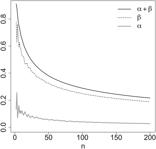
Table 2 shows the optimal adaptive averaged error probabilities α and β for various arm sizes without the restriction of the two arms having equal size. For a given total sample size, an unbalanced sample can have higher probabilities of both type-I and type-II errors than a balanced sample. For example, the error probabilities for an unbalanced sample with $n_1=60$ and $n_2=20$ are larger than those for a balanced sample with $n_1=n_2=40,$ even though both experiments would have the same total sample size, $n_1+n_2=80.$ The effect of unbalanced samples can be as important as the effect of total sample size. For example, the error probabilities of an unbalanced sample with $n_1=60$ and $n_2=10$ are larger than those of a balanced sample with $n_1=n_2=20,$ even though the unbalanced sample has a total size of $n_1+n_2=70$ and the balanced sample just 40.

Table 2 Optimal averaged error probabilities $\alpha ({\delta }^{*})$ and $\beta ({\delta }^{*})$ for comparison of two proportions for various arm sizes n₁ and n₂ in a two-arm medical study. Calculations were performed with a = b.

n1	n2	α	β	n1	n2	α	β	n1	n2	α	β
10	10	0.1639	0.4050	60	50	0.0626	0.2652	90	30	0.0707	0.2804
20	10	0.1318	0.3939	60	60	0.0591	0.2572	90	40	0.0648	0.2608
20	20	0.0995	0.3651	70	10	0.1130	0.3675	90	50	0.0575	0.2506
30	10	0.1159	0.3900	70	20	0.0865	0.3132	90	60	0.0550	0.2401
30	20	0.1045	0.3333	70	30	0.0727	0.2876	90	70	0.0529	0.2323
30	30	0.0997	0.3070	70	40	0.0645	0.2717	90	80	0.0493	0.2281
40	10	0.1250	0.3703	70	50	0.0603	0.2593	90	90	0.0468	0.2240
40	20	0.0868	0.3357	70	60	0.0575	0.2501	100	10	0.1111	0.3627
40	30	0.0850	0.3029	70	70	0.0539	0.2446	100	20	0.0818	0.3079
40	40	0.0706	0.2968	80	10	0.1130	0.3648	100	30	0.0684	0.2795
50	10	0.1126	0.3761	80	20	0.0834	0.3122	100	40	0.0617	0.2601
50	20	0.0883	0.3240	80	30	0.0704	0.2847	100	50	0.0559	0.2479
50	30	0.0767	0.2992	80	40	0.0634	0.2671	100	60	0.0538	0.2368
50	40	0.0718	0.2817	80	50	0.0603	0.2530	100	70	0.0512	0.2291
50	50	0.0667	0.2718	80	60	0.0553	0.2455	100	80	0.0483	0.2238
60	10	0.1097	0.3741	80	70	0.0531	0.2380	100	90	0.0467	0.2188
60	20	0.0860	0.3193	80	80	0.0508	0.2327	100	100	0.0449	0.2150
60	30	0.0765	0.2903	90	10	0.1131	0.3626
60	40	0.0689	0.2747	90	20	0.0810	0.3114

4.1.3 Test for One Proportion and the Likelihood Principle

A common example in which the Likelihood Principle can be violated is the comparison of binomials to negative binomials in a coin-flipping experiment with a coin that may or may not have the expected 50–50 chance of coming up “heads,” as described in Lindley and Phillips (1976).⁷ For the same values of x, the number of successes in n independent coin flips, the two distributions produce different p-values, which can lead to different decisions at a given level of significance. That is, the inference can actually be different for exactly the same data, depending on the intent of the researcher before starting the experiment. If a result is nine heads and three tails, did the researcher start the experiment planning to flip the coin exactly 12 times? Was the intent to flip until the 9th occurrence of heads? Until the third occorrence of tails? Was it some other intent, but the experiment was interrupted? With frequentist hypothesis tests, this actually matters because they violate the Likelihood Principle.

In this example, the new tests are applied to show that they do not violate the Likelihood Principle. The reason the inference (decision to accept or reject a hypothesis about the parameter θ) ends up being the same for different models is that although the P-values for the two models are different from each other, the adaptive significance levels α for the two models are also different, and the decision about rejecting one hypothesis in favor of the other ends up being the same. Using different notation from the previous example, let the sample vector consist of the number of successes x and the number of failures y, and let the corresponding vector of probabilities be $(\theta ,1-\theta ).$ Take $\mathbf{H}:\theta =\frac{1}{2}$ vs. $\mathbf{A}:\theta \ne \frac{1}{2},$ that is, a fair coin vs. an unbalanced coin, as the hypotheses to be tested. Taking a uniform prior for $\theta ,$ taking the two hypotheses to be equally probable a priori ($\pi =\frac{1}{2}$), and considering the two types of error equally severe, the predictive probabilities for the tests are as follows.

For a binomial,(12) $$f_{\mathbf{H}}(x,y)=\left(\begin{array}{c}x+y\\ x\end{array}\right){\left(\frac{1}{2}\right)}^{x+y}\hspace{1em}\text{and}\hspace{1em}{f}_{\mathbf{A}}(x,y)=\frac{1}{x+y+1},$$(12) and for a negative binomial,(13) $$\begin{array}{c}{f}_{\mathbf{H}}(x,y)=\left(\begin{array}{c}x+y-1\\ x\end{array}\right){\left(\frac{1}{2}\right)}^{x+y}\\ \hspace{1em}\text{and}\hspace{1em}{f}_{\mathbf{A}}(x,y)=\frac{y}{(x+y)(x+y+1)}.\end{array}$$(13)

The Bayes factors are equal for the two models, and since using the lemma will lead to comparing them to the same constant, the decisions about the hypothesis $\mathbf{H}:\theta =\frac{1}{2}$ end up being the same. The P-values and significance levels α are different for the two models, but the inference ends up being the same. Considering the observations $(x,y)=(3,10)$ and $(x,y)=(10,3)$ for a binomial, both samples yield the same results: $P=0.02,$ where the optimal error probabilities are $\alpha =0.09$ and $\beta =0.43.$ For a negative binomial, the same observations produce different values of the significance index P, but the error probabilities are different. For the first (second) sample, one stops observing when the number of successes reaches 3 (reaches 10). For the first sample point, the P-value is $0.01,$ and the relevant error probabilities are $\alpha =0.18$ and $\beta =0.48.$ For the second sample, $P=0.01,$ and the error probabilities are $\alpha =0.12$ and $\beta =0.33.$ The decisions made for binomials are the same as those for negative binomials with the same $(x,y).$ This behavior is much more general than this specific example, and in fact it is proven in Pereira et al. (2017) that the new tests are compliant with the Likelihood Principle for any discrete sample space.

4.1.4 An Important Note About “Yes–No” Experiments and the New Tests

The predictive densities under many common hypotheses in Bernoulli experiments can be calculated analytically for binomial and negative bionomial models when Beta priors are used. A few examples are ${\mathbf{H}}_1: \theta ={\theta }_0;$ ${\mathbf{H}}_2: \theta \ne {\theta }_0;$ ${\mathbf{H}}_3: \theta \le {\theta }_0$; ${\mathbf{H}}_4: \theta >{\theta }_0;$ ${\mathbf{H}}_5: \theta \in [{\theta }_1,{\theta }_2];$ and ${\mathbf{H}}_6: (\theta <{\theta }_1)\cup (\theta >{\theta }_2)$; etc. The predictive densities for several such sets of hypotheses are presented in Pereira et al. (2017).

4.2 Tests in Normal Distributions

Normal distributions are very widely used because the sample means of large random samples of random variables tend to act like normally distributed variables. This is the familiar tendency of large-sample distributions to look like “bell curves,” described mathematically by the central limit theorem. Details can be found in DeGroot (1986) or other statistics textbooks. Because of the importance of normal distributions, two examples are presented here of how the tests can be used with normal distributions.

4.2.1 Test of a Mean in a Normal Distribution

Consider iid variables $X_1,\dots ,X_n|\mu ,$ that obey a normal distribution with mean μ and variance 1. Take as a prior for μ a normal distribution with mean m and variance v. Instead of working with the full n-dimensional sample space, the minimal sufficent statistic ${\overline{X}}_n,$ the sample mean, can be used. The sampling distribution of ${\overline{X}}_n|\mu$ is a normal distribution with mean μ and variance $1/n$. For hypotheses $\mathbf{H}:\mu =0$ and $\mathbf{A}:\mu \ne 0$, the predictive distributions are ${\overline{X}}_n|\mathbf{H}\sim \mathcal{N}(0,1/n)$ and ${\overline{X}}_n|\mathbf{A}\sim \mathcal{N}(m,v+1/n)$.

To calculate the probability of a type-I error, define the region(14) $${\mathfrak{X}}_{\mathbf{A}}=\{{\overline{x}}_n:f_{\mathbf{H}}({\overline{x}}_n)/f_{\mathbf{A}}({\overline{x}}_n)<1\},$$(14) and evaluate $\alpha ={\int }_{{\mathfrak{X}}_{\mathbf{A}}}{f}_{\mathbf{H}}({\overline{x}}_n) \mathrm{d}{\overline{x}}_n$. For the probability of a type-II error, define the region ${\mathfrak{X}}_{\mathbf{H}}=\{{\overline{x}}_n:f_{\mathbf{H}}({\overline{x}}_n)/f_{\mathbf{A}}({\overline{x}}_n)>1\}$, and evaluate $\beta ={\int }_{{\mathfrak{X}}_{\mathbf{H}}}{f}_{\mathbf{A}}({\overline{x}}_n) \mathrm{d}{\overline{x}}_n$. 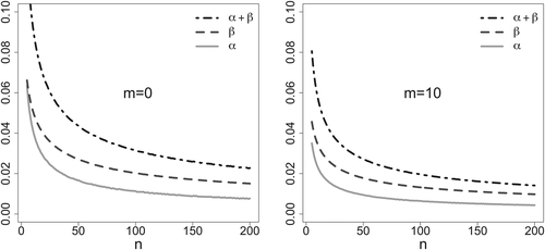These error probabilities are plotted in Figure 2 for v = 100 and two values of the prior mean: m = 0 and $m=10.$ The plot with m = – 10 would be identical to the plot with m = 10.

Fig. 2 Type-I (solid gray lines), type-II (dashed black lines), and total (dot-dashed black lines) error probabilities as functions of sample size n for tests of $\mathbf{H}:\mu =0$ on a normally distributed variable with variance 1 and unknown mean $\mu , \mathcal{N}(\mu ,1),$ with priors for the mean $\mu \sim \mathcal{N}(m,100)$ with m = 0 (left) and m = 10 (right).

4.2.2 Test of a Variance in a Normal Distribution

This is an example used by Pereira and Wechsler (1993), showing that the region of the space of possible results where a test rejects the null hypothesis is not always the tails of the null distribution; it can be a union of disjoint intervals. In such cases, it can be impossible to calculate a classical p-value defined as in Definition 1, but the ordering of the entire sample space by Bayes factors allows for an unambiguous definition and calculation of the new index, a capital-P P-value in the sense of Definition 2.

Consider a normally distributed random variable X with mean zero and unknown variance ${\sigma }^2.$ The hypotheses considered here are $\mathbf{H}: {\sigma }^2=2$ and $\mathbf{A}: {\sigma }^2\ne 2.$ A ${\chi }_1^2$ (chi-squared with one degree of freedom) distribution is used as a prior density for ${\sigma }^2.$ The predictive densities under hypotheses H and A are(15) $$f_{\mathbf{H}}\left(x\right)=\frac{1}{2\sqrt{\pi }}\text{exp}\hspace{0.17em}\left(-\frac{x^2}{4}\right) \text{and} f_{\mathbf{A}}\left(x\right)=\frac{1}{\pi \left(1+x^2\right)},$$(15) a normal density with mean zero and variance 2, and a Cauchy density, respectively. Figure 3 shows a plot of the Bayes factor, using a value of 1.1 as a cutoff for a decision about the hypotheses. The sample points that do not favor H are in three separate regions: a central interval and the heavy tails of the Cauchy density. The set that favors H is the complement, made up of two intervals between the central interval and the tails:(16) $$X_{\mathbf{H}}=\left\{x\right|x\in (-2.8,-0.6)\cup (0.6,2.8)\}.$$(16)

Fig. 3 Bayes factor for $\mathcal{N}(0,2)$ vs. Cauchy, arising from a test of a normal variance with hypotheses $\mathbf{H}: {\sigma }^2=2$ vs. $\mathbf{A}:{\sigma }^2\ne 2$.

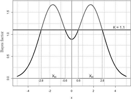
The set that favors A over H includes, in addition to the tails, the central region $(-0.6,0.6).$ Even with this or even more complex divisions of the sample space into regions that favor one hypothesis over another, the new method allows for calculation of a P-value.

4.3 Test of Hardy–Weinberg Equilibrium

“Hardy–Weinberg equilibrium” refers to the principle, proven by Hardy (1908) and Weinberg (1908), that allele and genotype frequencies in a population will remain constant from generation to generation, given certain assumptions about the absence of external evolutionary influences.

An individual’s genotype is determined by a combination of alleles. If there are two possible alleles for some characteristic (say A and a), the possible genotypes are AA, Aa, and aa. Let $x_1,x_2,x_3$ be the observed frequencies of the genotypes AA, Aa, and aa, respectively, and ${\theta }_1,{\theta }_2,{\theta }_3$ the corresponding probabilities. Assuming a few premises, as described by Hartl and Clark (1989), the principle says that the allele probabilities in a population do not change from generation to generation. It is a fundamental principle for the Mendelian mating allelic model. If the probabilities of alleles are θ for allele A and $1-\theta$ for the allele a, the expected genotype probabilities are $\left(({\theta }^2,2\theta (1-\theta ),{(1-\theta )}^2\right),0\le \theta \le 1$.

The Hardy–Weinberg equilibrium hypothesis is(17) $$\mathbf{H}:\{\begin{array}{ccc}{\theta }_1& =& {\theta }^2,\\ {\theta }_2& =& 2\theta (1-\theta ),\\ {\theta }_3& =& {(1-\theta )}^2,\end{array}$$(17)

Given n, using as a prior distribution for $\{{\theta }_1,{\theta }_2,{\theta }_3\}$ a Dirichlet(1, 1, 1), that is, $f({\theta }_1,{\theta }_2,{\theta }_3)=2$, and using the multinomial probability(18) $$f(x_1,x_2,x_3|{\theta }_1,{\theta }_2,{\theta }_3)=\frac{n!}{x_1!x_2!x_3!}{\theta }_1^{x_1}{\theta }_2^{x_2}{\theta }_3^{x_3}$$(18) for $(x_1,x_2,x_3),$ the predictive under hypothesis A is(19) $$\begin{array}{c}{f}_{\mathbf{A}}(x_1,x_2,x_3)={\int }_0^1{\int }_0^{1-{\theta }_1}f(x_1,x_2,x_3|{\theta }_1,{\theta }_2,1-{\theta }_1-{\theta }_2)\\ \hspace{1em}\times f({\theta }_1,{\theta }_2,1-{\theta }_1-{\theta }_2)\mathrm{d}{\theta }_1\mathrm{d}{\theta }_2\\ ={\int }_0^1{\int }_0^{1-{\theta }_1}\frac{n!}{x_1!x_2!x_3!}{\theta }_1^{x_1}{\theta }_2^{x_2}{(1-{\theta }_1-{\theta }_2)}^{x_3}\\ \hspace{1em}\times 2 \mathrm{d}{\theta }_1\mathrm{d}{\theta }_2\\ =\frac{2n!}{(n+2)!}.\end{array}$$(19)

Under hypothesis H, the surface integral to normalize the values of the prior density in the set corresponding to the null hypothesis yields $f(\theta )=1,0\le \theta \le 1$. Then,(20) $$\begin{array}{cc}{f}_{\mathbf{H}}(x_1,x_2,x_3)\hfill & ={\int }_0^{1}f(x_1,x_2,x_3|\theta \left)f\right(\theta ) \mathrm{d}\theta \hfill \\ \hfill & ={\int }_0^1\frac{n!}{x_1!x_2!x_3!}{2}^{x_2}{\theta }^{2x_1+x_2}{(1-\theta )}^{2x_3+x_2} \mathrm{d}\theta \hfill \\ \hfill & =\frac{n!2^{x_2}(2x_1+x_2)!(2x_3+x_2)!}{x_1!x_2!x_3!(2n+1)!}.\hfill \end{array}$$(20)

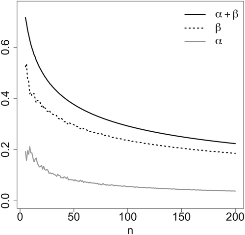
The probability of a type-I error, $\alpha ,$ is obtained from a sum of the predictive under H over all samples $\{x_1,x_2,x_3\}$ where $f_{\mathbf{H}}(x_1,x_2,x_3)/f_{\mathbf{A}}(x_1,x_2,x_3)<1.$ The probability of a type-II error, $\beta ,$ is obtained from a sum of the predictive under A over all samples $\{x_1,x_2,x_3\}$ where $f_{\mathbf{H}}(x_1,x_2,x_3)/f_{\mathbf{A}}(x_1,x_2,x_3)>1$. These error probabilities are plotted in Figure 4.

Fig. 4 Type-I (solid gray line), type-II (dotted line), and total (solid black line) error probabilities as functions of the sample size n for the Hardy–Weinberg equilibrium hypothesis.

5 Final Considerations

Using the hypothesis-testing procedure described here, the sample-size dependence of the optimal averaged α can be used to determine the best significance level for a given n, which can be relevant in studies where a limited number of trials can be done, or to determine the necessary sample size to achieve a desired $\alpha .$

The procedure can be applied to other models and hypotheses, without restrictions on the dimensionality of the parameter space or the sample space. The sample space, regardless of its dimensionality, is ordered by a single real number, the Bayes factor. In all the examples used in this article, analytic (closed-form mathematical) solutions are available, but this is not the case for all distributions and hypotheses. For example, hypotheses about a normal distribution with unknown mean and variance involve calculations of significantly greater complexity and require some sort of analytic approximations or approximate methods for evaluating the necessary integrals, such as Monte Carlo methods. Note that the method requires the calculation of five integrals: two over the nuisance parameter(s) to find the predictive distributions $f_{\mathbf{H}}(x)$ and $f_{\mathbf{A}}(x);$ and three of predictive distributions over specific regions of the sample space to obtain $\alpha ,$ $\beta ,$ and the capital-P P-value.

It is worth noting that the approach described here is compatible with guidelines in the ASA’s statement on p-values (Wasserstein and Lazar (2016)). Specifically, because the signficance level depends on the sample size, and therefore is not the kind of predefined “bright-line” rule the ASA recommends avoiding, the approach is compatible with point 3, “Scientific conclusions and business or policy decisions should not be based only on whether a p-value passes a specific threshold.”

Funding

Acknowledgement

The authors thank Dr. Ronald L. Wasserstein for encouragement to write this article and Dr. Sergio Wechsler for illuminating conversations about the research described here and his invaluable contributions to research that led to the present work.

Notes

Additional information

Funding

This study was financed in part by Coordenação de Aperfeiçoamento de Pessoal de Nível Superior - Finance Code 001. C.A. de B.P. thanks the Conselho Nacional de Desenvolvimento Científico e Tecnológico, CNPq, for support under grant number 308776/2014-3.

Notes

1 Fisher’s tests do not require the null to be a “nil,” but tests are usually performed that way, even in Fisher’s own work.

2 Some readers may be familiar with the power of a test, the probability of correctly rejecting a false null hypothesis. The power of a test is given by $1-\beta .$

3 A likelihood function corresponding to a given probability (density) function is given by the same expression, but taken as a function of the parameter θ for a fixed value of the observation x. In general, a probability (density) function for any given value of the parameter $\theta ,$ summed (integrated) over the entire space of all possible observations, yields 1, while the corresponding likelihood for a given observation x may not even be summable (integrable) over the entire space of all possible parameter values, much less yield the specific value 1.

4 The definition numbers 2.2 and 2.1 from Pereira and Wechsler (1993) are maintained, even though they are presented in the opposite order in this article.

5 A proof of the equivalence of the LP to the combination of two much less-controversial principles, the Conditionality Principle (CP) and Sufficiency Principle (SP), appears in Birnbaum (1962), and a modified version in Wechsler, Pereira, and Marques (2008), but the validity of this kind of proof has been questioned by, for example, Evans (2013) and Mayo (2014). Gandenberger (2015) presents a proof of the same equivalence designed to resist the kinds of attacks brought against Birnbaum’s proof, but the controversy continues to rage. It is worth noting that even if both proofs were incorrect, that would not mean that the LP was not equivalent to the combination of the CP and SP. Further, even if that equivalence were not valid, that would not mean that the LP is not true. Even so, the LP is still not considered proved, which is why it is still just a principle that one chooses either to accept or not.

6 The notation “probability (density) function” is used to refer to a probability function for discrete sample spaces and a probability density function for continuous sample spaces.

7 Lindley and Phillips actually consider throws of thumbtacks, called “drawing pins” in U.K. English, but the principle is identical.

References

- Bartlett, M. (1957), “A Comment on D. V. Lindley’s Statistical Paradox,” Biometrika, 44, 533–534. DOI:10.1093/biomet/44.3-4.533.
- Benjamin, D. J., Berger, J. O., Johannesson, M., Nosek, B. A., Wagenmakers, E. J., Berk, R., Bollen, K. A., Brembs, B., Brown, L., Camerer, C., Cesarini, D., Chambers, C. D., Clyde, M., Cook, T. D., De Boeck, P., Dienes, Z., Dreber, A., Easwaran, K., Efferson, C., Fehr, E., Fidler, F., Field, A. P., Forster, M., George, E. I., Gonzalez, R., Goodman, S., Green, E., Green, D. P., Greenwald, A. G., Hadfield, J. D., Hedges, L. V., Held, L., Hua Ho, T., Hoijtink, H., Hruschka, D. J., Imai, K., Imbens, G., Ioannidis, J. P. A., Jeon, M., Jones, J. H., Kirchler, M., Laibson, D., List, J., Little, R., Lupia, A., Machery, E., Maxwell, S. E., McCarthy, M., Moore, D. A., Morgan, S. L., Munafó, M., Nakagawa, S., Nyhan, B., Parker, T. H., Pericchi, L., Perugini, M., Rouder, J., Rousseau, J., Savalei, V., Schönbrodt, F. D., Sellke, T., Sinclair, B., Tingley, D., Van Zandt, T., Vazire, S., Watts, D. J., Winship, C., Wolpert, R. L., Xie, Y., Young, C., Zinman, J., and Johnson, V. E. (2018), “Redefine Statistical Significance,” Nature Human Behaviour, 2, 6–10. DOI:10.1038/s41562-017-0189-z.
- Berger, J., and Wolpert, R. (1988), The Likelihood Principle, (2nd ed.), Haywood, CA: The Institute of Mathematical Statistics, available at https://projecteuclid.org/euclid.lnms/1215466210
- Berger, J. O., and Delampady, M. (1987), “Testing Precise Hypotheses,” Statistical Science, 2, 317–335. DOI:10.1214/ss/1177013238.
- Birnbaum, A. (1962), “On the Foundations of Statistical Inference,” Journal of the American Statistical Association, 57, 269–306. DOI:10.1080/01621459.1962.10480660.
- Cohen, J. (1994), “The Earth is round (p <.05),” American Psychologist, 49, 997–1003.
- Cornfield, J. (1966), “Sequential Trials, Sequential Analysis and the Likelihood Principle,” The American Statistician, 20, 18–23. DOI:10.1080/00031305.1966.10479786.
- DeGroot, M. (1986), Probability and Statistics, Addison-Wesley Series in Statistics, Reading, MA, USA: Addison-Wesley Publishing Company. DOI:10.1086/ahr/80.1.64.
- Evans, M. (2013), “What does the Proof of Birnbaum’s Theorem Prove?” Electronic Journal Statistics, 7, 2645–2655. DOI:10.1214/13-EJS857.
- Gandenberger, G. (2015), “A New Proof of the Likelihood Principle,” The British Journal for the Philosophy of Science, 66, 475–503. DOI:10.1093/bjps/axt039.
- Gelman, A. and Rubin, D. B. (1995), “Avoiding Model Selection in Bayesian Social Research,” Sociological Methodology, 25, 165–173. DOI:10.2307/271064.
- Hardy, G. H. (1908), “Mendelian Proportions in a Mixed Population,” Science, 28, 49–50. DOI:10.1126/science.28.706.49.
- Hartl, D. L. and Clark, A. G. (1989), Principles of Population Genetics, (2nd ed.), Sunderland, Mass.: Sinauer Associates.
- Jeffreys, H. (1935), “Some Tests of Significance, Treated by the Theory of Probability,” Mathematical Proceedings of the Cambridge Philosophical Society, 31, 203–222. DOI:10.1017/S030500410001330X.
- Jeffreys, H. (1939), The Theory of Probability, Oxford: The Clarendon Press.
- Kass, R. E., and Raftery, A. E. (1995), “Bayes Factors,” Journal of the American Statistical Association, 90, 773–795. DOI:10.1080/01621459.1995.10476572.
- Levine, T. R., Weber, R., Hullett, C., Park, H. S., and Lindsey, L. L. M. (2008), “A Critical Assessment of Null Hypothesis Significance Testing in Quantitative Communication Research,” Human Communication Research, 34, 171–187. DOI:10.1111/j.1468-2958.2008.00317.x.
- Lindley, D. V. (1957), “A Statistical Paradox,” Biometrika, 44, 187–192. DOI:10.1093/biomet/44.1-2.187.
- Lindley, D. V., and Phillips, L. D. (1976), “Inference for a Bernoulli Process (a Bayesian View),” The American Statistician, 30, 112–119. DOI:10.2307/2683855.
- Mayo, D. G. (2014), “On the Birnbaum Argument for the Strong Likelihood Principle,” Statistical Science, 29, 227–239. DOI:10.1214/13-STS457.
- Montoya-Delgado, L. E., Irony, T. Z., Pereira, C. A. B., and Whittle, M. R. (2001), “An Unconditional Exact Test for the Hardy-Weinberg Equilibrium Law: Sample-Space Ordering Using the Bayes Factor,” Genetics, 158, 875–883.
- Neyman, J., and Pearson, E. S. (1933), “On the Problem of the Most Efficient Tests of Statistical Hypotheses,” Philosophical Transactions of the Royal Society of London. Series A, Containing Papers of a Mathematical or Physical Character, 231, 289–337. DOI:10.1098/rsta.1933.0009.
- Pereira, C. A. d. B., Nakano, E. Y., Fossaluza, V., Esteves, L. G., Gannon, M. A., and Polpo, A. (2017), “Hypothesis Tests for Bernoulli Experiments: Ordering the Sample Space by Bayes Factors and Using Adaptive Significance Levels for Decisions,” Entropy, 19, 696. DOI:10.3390/e19120696.
- Pereira, C. A. d. B., and Wechsler, S. (1993), “On the Concept of p-value,” Revista Brasileira de Probabilidade e Estatística, 7, 159–177.
- Pericchi, L., and Pereira, C. (2016), “Adaptative Significance Levels using Optimal Decision Rules: Balancing by Weighting the error Probabilities,” Brazilian Journal of. Probability and Statistics, 30, 70–90. DOI:10.1214/14-BJPS257.
- Schervish, M. (2012), Theory of Statistics, Springer Series in Statistics, New York: Springer.
- Trafimow, D., and Marks, M. (2015), “Editorial,” Basic and Applied Social Psychology, 37, 1–2. DOI:10.1080/01973533.2015.1012991.
- Tukey, J. W. (1969), “Analyzing Data: Sanctification or Detective Work?” American Psychologist, 24, 83–91. DOI:10.1037/h0027108.
- Wasserstein, R. L., and Lazar, N. A. (2016), “The ASA’s Statement on p-Values: Context, Process, and Purpose,” The American Statistician, 70, 129–133. DOI:10.1080/00031305.2016.1154108.
- Weakliem, D. L. (1999), “A Critique of the Bayesian Information Criterion for Model Selection,” Sociological Methods & Research, 27, 359–397. DOI:10.1177/0049124199027003002.
- Wechsler, S., Pereira, C. A. d. B., and Marques F., P. C. (2008), “Birnbaum’s Theorem Redux,” in Bayesian Inference and Maximum Entropy Methods in Science and Engineering: Proceedings of the 28th International Workshop, eds. de Souza Lauretto, M., de Bragança Pereira, C. A., and Stern, J. M., American Inst. of Physics, pp. 96–102.
- Weinberg, W. (1908), “Über den Nachweis der Vererbung beim Menschen,” Jahreshefte des Vereins für vaterländische Naturkunde in Württemberg, 64, 369–382.