Quality Control for Scientific Research: Addressing Reproducibility, Responsiveness, and Relevance

ABSTRACT

Efforts to address a reproducibility crisis have generated several valid proposals for improving the quality of scientific research. We argue there is also need to address the separate but related issues of relevance and responsiveness. To address relevance, researchers must produce what decision makers actually need to inform investments and public policy—that is, the probability that a claim is true or the probability distribution of an effect size given the data. The term responsiveness refers to the irregularity and delay in which issues about the quality of research are brought to light. Instead of relying on the good fortune that some motivated researchers will periodically conduct efforts to reveal potential shortcomings of published research, we could establish a continuous quality-control process for scientific research itself. Quality metrics could be designed through the application of this statistical process control for the research enterprise. We argue that one quality control metric—the probability that a research hypothesis is true—is required to address at least relevance and may also be part of the solution for improving responsiveness and reproducibility. This article proposes a “straw man” solution which could be the basis of implementing these improvements. As part of this solution, we propose one way to “bootstrap” priors. The processes required for improving reproducibility and relevance can also be part of a comprehensive statistical quality control for science itself by making continuously monitored metrics about the scientific performance of a field of research.

KEYWORDS:

• p-Values
• Process control
• Relevance
• Replication
• Reproducibility

1 Introduction

The failure of researchers to reproduce statistical results in many different disciplines has led to what we know as the reproducibility crisis.¹ The reasons for the difficulty to reproduce results include sample deficiencies and low power, incorrect application and interpretation of statistical tests and misalignment of data with research questions (Stodden 2015; Hubbard 2016). The reluctance of researchers to share data and code contributes to the reproducibility crisis as well, since it is often difficult to reproduce the exact statistical analysis without access to the software that was used to produce the original results (e.g., Stodden 2013). This is not a new problem; as early as 1935, Fisher mentioned the need for replication for scientific validity, an idea repeated in Popper (1959). Sterling (1959), Rosenthal (1979), and Sackett (1979) discussed the effect of publication bias on reproducibility in various scientific disciplines over 50 years ago. Dickersin (1990) revisited the question of publication bias in the context of medical research. Buckheit and Donoho (1995) pioneered the concept of open-access software and datasets to address the issue of reproducibility, using as an example a suite of programs developed by them to analyze images. Casadevall and Fang (2010) present a good discussion about reproducible science.

In recent years, the pace at which articles in the peer-reviewed literature and in the popular literature have been published has increased tremendously. Even after warnings as early as Fisher’s, decades pass as evidence mounts with no fundamental change in how statistical inference methods are applied.

The Manifesto for Reproducible Science (Munafó et al. 2017) thoroughly describes the problem with replication in certain areas of science and it brings together multiple valid suggestions from many authors for making improvements. Among other suggestions, the manifesto promotes research registries, better statistical training and transparency of data to reduce problems like publication bias, p-hacking, and HARKING. Publication bias occurs when the chance that the work is published depends not only on its quality but also on the outcome of the research. Therefore, projects that have a statistically significant result have a larger probability of being submitted and published (e.g., Dickersin 1990). The term p-hacking is used to describe the situation where a researcher tests all possible hypotheses or uses the subset of the data to obtain statistically significant results (Goodman 1999). HARKing stands for “hypothesis after results are known” and is related to the idea of p-hacking. A good reference is Kerr (1998). Munafó et al. (2017) do not propose any significant change to the statistical inference methods themselves and they assume the continued reliance of existing methods like p-values and null hypothesis significance testing (NHST). In fact, in our view, many researchers interested in the problems of reproducibility, appear to see the problem as primarily one of the incorrect use of p-values and NHST, not the reliance on these methods themselves, correctly used or not.

The incorrect use of NHST surely has something to do with reproducibility. Perhaps one of the most common misunderstandings, for example, is that a p-value is an estimate of the probability that the null hypothesis is true. Instead, the p-value is actually defined as the probability of observing a statistic as or more extreme than the one we obtained, when the null hypothesis is true. Used correctly, p-values can be useful as part of the measure of the discrepancy of the data and the null hypothesis, recent negative press notwithstanding. This said, the correct use of NHST alone does not address reproducibility because it does not address publication bias. It also does not address two other issues which need to be resolved together with reproducibility: relevance and responsiveness.

The issue of relevance refers to answering the right question: given the data, what is the probability that a hypothesis is true? The most important and difficult decisions by either corporate or government policy makers are virtually always made under some state of uncertainty. A systematic approach to making decisions under uncertainty is formally described in the fields of decision analysis and utility theory and these methods also have practical applications. In these fields, a fundamental requirement of making decisions under uncertainty is assigning probabilities to possible outcomes. The p-value and NHST alone do not and, in fact, cannot be sufficient for computing the required probabilities on outcomes.

The issue of responsiveness refers to how quickly systematic problems in research are detected and corrected. The relatively recent publication by Ioannidis (2005) provocatively titled “Why Most Published Research Findings are False” would apply to research that goes back decades. Even when problems with one or more studies are found, corrections can take years. Additional reproducibility research on psychology studies was conducted seven years after the publication dates of the original studies (Open Science Collaborative 2015). Reproducibility will likely continue to be a problem if the detection and subsequent corrective actions have such delays. Delays on this scale in the detection and correction of problems would surely be untenable in manufacturing and other areas of business and government.

The solution to the problem of responsiveness requires continuous “statistical process control” for science itself. One component of this approach is to compute a baseline “prior” probability for a field. The baseline prior for a field of study (e.g., childhood nutrition, clinical psychology, etc.) is the probability that the hypothesis being tested in a randomly selected proposed study is true. We will show the surprising finding that such a prior can be derived from knowing only the power, significance level and past reproduction study results from a set of studies in a particular field. This, together with controls prescribed by others (e.g., The Manifesto for Reproducible Science) may be a solution for improving the overall quality and usefulness of scientific research.

Before we introduce the approach to carry out quality control of scientific research that we propose, we note that not everyone believes that there is a reproducibility crisis in scientific research. In a recent publication, Jager and Leek (2014) dispute the notion that the reproducibility crisis in medical studies is as dire as it is in other scientific areas. The authors reviewed every manuscript published in the major medical journals between 2000 and 2010, and found that among the 5200 papers that included p-values, the false discovery rate was estimated to be no larger than $14\pm 1\%$. Jager and Leek then conclude that the medical literature continue to provide an adequate record of real scientific progress.

2 An Argument for Priors

2.1 Decision Making Under Uncertainty

Assigning probabilities to outcomes from alternative courses of action is fundamental in the context of making decisions in virtually every field where decisions under uncertainty is analyzed quantitatively. This includes game theory and decision theory, operations research, quantitative portfolio management, and actuarial science. We would argue that even for decision makers who may not explicitly state probabilities of outcomes, this is at least an intuitive consideration for many of them. When a company invests in developing a new product, when an insurance company computes a premium, or when an entrepreneur starts a business, there is at least an implicit belief that some outcomes are more likely than others. Of course, this has been acknowledged by many previous authoritative sources so, instead of repeating their entire arguments here, we will select a few of their most salient statements on this point. For one, an early and perhaps most influential work in decision theory (Von Neumann and Morgenstern 1944) consider this fundamental to making decisions under uncertainty when they said the following:

We have assumed only one thing, and for this there is good empirical evidence, namely that imagined events can be combined with probabilities. And, therefore, the same must be assumed for the utilities attached to them, whatever they may be.

Von Neuman and Morgenstern repeated throughout their work similar points about the necessity of assigning probabilities to all possible outcomes. Others who find priors an unavoidable necessity for decisions include Savage (1954), Wald (1950), Jaynes (1958), and—more recently—Howard (1977, 1984, 2015). If we accept the positions of individuals like these on the need for assigning probabilities to outcomes, it should also be clear that to do that we must state prior probabilities. As Jaynes put it as early as 50 years ago, the argument was sufficiently convincing to conclude “priors could no longer be ignored.”

Priors can be anything from a highly individual notion about “the states of nature” to a naïve, standardized prior. We argue below that we can think of priors at different levels, and that at each level, the prior would reflect a different amount of information. (Each level is effectively a posterior probability relative to the previous level and a prior to the next.) Of course, the users of the study or future researchers do not have to accept the stated prior. On the contrary, we are proposing that we limit restrictions on users of research results, as well as on future researchers, by providing many options for the analysis of the data. First and foremost among these, is the option to have access to all of the research data as recommended in the Manifesto. But even if this access to data is provided—and especially if it is not—researchers should provide users and future researchers multiple methods of analyses of these data. As the previously quoted sources would surely agree, researchers should also provide a recommended prior and the resulting posterior probabilities for any hypothesis in the study. We address the question of constructing these priors in subsequent sections. We also recommend providing Bayes factors (BFs) especially if, for any reason, the access to data and priors is not provided. And none of this needs to displace conventional test results such as p-values. Providing this much analytical detail is possible (but perhaps not trivial) when we fully exploit the era of “post-print” (i.e., digital, online) media for publishing scientific research. In such an environment, the practical data limitations of printed and bound issues can be ignored and inferences can be dynamically updated with replication studies and other data.

2.2 The Probability That a Study’s Results Are True

So now, we proceed as if the reader has reviewed the arguments of those like Savage and Von Neuman and has ultimately accepted them. In the Bayesian context, prior distributions are used to summarize knowledge about “the state of nature” (often represented in the form of a parameter such as a mean or the probability of occurrence of some event) before any data are collected. Once data become available from an experiment or by some other means, prior information is combined with the information provided by the data using Bayes’ rule. Bayes’ rule establishes that the posterior odds in favor of a hypothesis equals the product of the prior odds and the likelihood ratio. The rule is prescriptive, and its application results in a posterior distribution that reflects all of the information about the parameter that is available to the investigator. The posterior distribution is simply the distribution of likely values of the parameter given the data, and can be thought of as the updated prior distribution after the data have been observed.

A rich literature argues that the Bayesian approach is rational and coherent, but even after the strong cases made by these early authors on the topic, there is one persistent objection to the use of priors in scientific inference. This objection is based on the idea that objectivity is preferable to the lack of it, that significance tests are “objective” and that the use of priors is merely “subjective.” The claimed objectivity of p-values and significance tests was asserted and reasserted to researchers in their earliest statistics courses while challenges to this claim, it seems, are not given the same exposure. We agree with Jaynes (2003) on the confusion in the objectivity versus subjectivity distinction when he observed that “These words are abused so much in probability theory that we try to clarify our use of them.”

The word “objectivity” itself bears some analysis. There are two specific meanings of this word that are often conflated when applied to tests of significance. In one sense, objective is used as having reality independent of the mind (as in “objective reality”). Used this way, an arbitrary standard of human creation like p < 0.05 is not “objective.” In another sense, objective is used to mean “impartial”—that is, unbiased and equal treatment by a judge, arbitrator, or referee. Taken further, impartiality means that different people would have gotten the same answer when the same inputs are provided. Even Fisher (1973), certainly not known for being an advocate of priors in statistical inference, appeared to use it in this latter sense when he said

$\dots$ the feeling induced by a test of significance has an objective basis in that the probability statement on which it is based is a fact communicable to, and verifiable by, other rational minds.

It is in this latter sense, the same sense used by Fisher, that the word “objective” applies to significance tests. But in this latter more relevant sense, objectivity is not an exclusive feature of significance levels. Priors are just as objective in this sense.

If either a prior or significance level are stated as an explicit, impartial assumption, then a mathematically correct calculation subsequent to it is objective in this latter sense. For example, the statement “if we assume $\text{Pr}(X)=0.05, \text{Pr}(Y)=0.5$, and $\text{Pr}(X|Y)=0.5$, then $\text{Pr}(Y|X)=0.05$” is necessarily true regardless of how we determined $\text{Pr}(X), \text{Pr}(Y)$, and $\text{Pr}(X|Y)$, subjectively or not. Furthermore, if an independent reviewer or other entity (i.e., not the researcher) is the source of the assumption $\text{Pr}(X)=0.05$, then the entire statement is as impartial as a significance level used as a matter of convention for a field of research. Used in this sense, mathematically correct statements containing assumed but impartial priors are just as objective as a statement containing an assumed and impartial significance level. In fact, the researcher using a significance test should and often does state caveats like “using a significance level of 0.05” or “assuming $\alpha <0.05$” before reporting whether they reject of fail to reject the null hypothesis.

3 Do Decisions Require the “Rejection” or “Acceptance” of a Hypothesis?

Since the beginning of statistical tests, there has been an implied need to use arbitrary thresholds as a the basis for acceptance or rejection of some hypothesis, as if evidence for a claim could be best summarized by sorting claims into one of the two buckets of “accept” or “reject.” In the case of the significance test that compares the p-value with some α-level, some go further by defining multiple Type I error levels such as $\alpha =0.05,\alpha =0.01,\alpha =0.001$. Researchers may often indicate when p-values meet these significance levels with one, two, or three asterisks, respectively.

Such discretization is not needed and is bad for decision making. Discrete, universally applied thresholds simply do not appear in various quantitative fields related to decision making under uncertainty. One such field, decision analysis, is the practical application of decision theory for decision making under uncertainty (Von Neumann and Morgenstern 1944; Howard and Matheson 1977, 1984; Howard and Abbas 2015). At no point in decision analysis does the “count of asterisks” become a variable in optimizing a decision. Other practical (and highly overlapping) analytical fields, such as actuarial science, management science, and operations research also do not depend on such distinctions. In these approaches, optimal decision making is modeled as a function of consequences of outcomes of alternatives and the probability distributions over those outcomes. If the possible rewards for a given action are large enough compared to losses, the action may be desirable even if the probability of the reward is low. If, for example, the methods of decision theory were the basis of health policy decisions, the adoption of a new, very expensive disease treatment with serious side effects may require a higher probability of a large benefit than is required for the adoption of a treatment which is less expensive, with fewer side effects, for a fatal condition with no other treatment.

One possible advantage of moving away from discretized, arbitrary thresholds is that apparently lukewarm findings may provide some incentive for replication. After all, the need to reproduce has probably seemed like a low priority once a researcher determines an effect to be “significant.” The phrase “statistically significant” may give the typical user of the research the idea that they can be very confident in the results and that further research is not justified. But if $\text{Pr}(H| \text{data})=0.43$, then maybe it will seem more clear that the research is not yet over. As we are about to show, posterior probabilities of that magnitude may be the norm for much of the published research in the social sciences. And, of course, whether or not a finding is statistically significant does not by itself confirm whether it is likely to be true, whether an effect is clinically important, or even whether it is worthy of further study. At no point do counts of asterisks or thresholds like “high” or “significant” come into consideration.

4 Levels for Constructing Priors

We propose three possible levels in which we generate priors.

• Level 0 Arbitrary, uninformed, universal prior: In this level, we would use a single prior, set as an arbitrary convention for any hypothesis in an entire field, in much the same way that P < 0.05 has been used as the threshold de jure or de facto for statistical significance. Of course, even this conventional prior can be used in a perfectly objective way when, as previously argued, it is stated as an explicit caveat such as “If we assume $P(H)=0.05$, then $P(H| \text{data})=0.45$.” However, we consider this to be an extremely rudimentary approach which provides no advantage over conventional significance levels. We propose that more advanced levels should be pursued.

• Level 1 Informed universal prior: If replication studies in a given field become available, then the prior for any single hypothesis in an entire field can be informed. To do so, we treat the previous replications themselves as a sample of the population of potential research in a field. This could be used to produce a kind of “implied prior” consistent with observed replication rates. We will show a simple example of how this can be done in Section 5.

• Level 2 Discriminated prior: To derive a discriminated prior for specific research studies, we need additional, study-level information. For example, it has been shown that the sponsor of research has bearing on the replication success (e.g., Rochon et al. 1994; Friedberg et al. 1999). This and other factors can be considered to differentiate priors among different studies. The Level 2 prior can also be informed by the judgment of experts. We will review some potential methods.

As just mentioned, Level 0 prior would be a trivial but not recommended solution. Using an arbitrary threshold defined by convention is essentially what the current use of a significance levels does. Level 0 would not be an improvement, although it would not be worse, either (both are equally “objective”). So we will start with how a Level 1 solution to produce priors could be estimated.

Like Level 0, Level 1 produces a single prior for an entire field of research (i.e., the prior does not discriminate among different proposed research studies). Unlike Level 0, Level 1 is an informed prior based on previous replication studies in a given research field. The challenge is to infer this from previous replication studies which, themselves, relied on conventional significance tests. The prescribed approach asks “what is the prior that would be most consistent with observed replication rates?” If an initial Level 1 prior is estimated for a given field and if priors and posteriors will be used from then on (instead of conventional significance tests), the following method may no longer need to be employed.

5 Constructing a Level 1 Prior

We begin by framing a population for which inferences will be made by using a sample from the population. Consider a set of all potential research studies in a field. We leave it to researchers to define what constitutes their fields as they see fit. A “field” could be defined by existing professional bodies and institutions or may be all the articles submitted to a particular publication.²

We can think of a field as a set of research studies proposed by some body of researchers. Only a subset of these proposed studies have been conducted to date. That is, studies conducted so far are a sample of the population of studies potentially proposed by the researchers of a field. Furthermore, unless we have reason to believe that there is some order to which studies are conducted first, we propose to treat the studies conducted to date as a random sample of the population. Note that this is not an assumption about whether topics of research will change over time. Of course, that will change but that, too, can be part of computing the prior for a field. It is only a proposed starting point unless and until future observations show otherwise. We do not wish to suggest that converting these ideas into practice is without difficulty.

Also, we treat reproduction studies as a random sample of studies that were published. Here, by replication studies we refer to studies that address the same or a sufficiently similar issue as the original study. If we can make an estimate of the distribution of “true hypothesis” in the population of potential studies, then we use that as the prior for a subsequent proposed study (which, again, we treat as being randomly selected from the population of potential studies).

Now consider the simplest situation where a proposition H is either true or false (we will ignore the question of effect size for now). Suppose that in a given field hundreds of such propositions have been researched and published over the years in the peer-reviewed literature, and suppose further that we are interested in investigating the overall quality of this body of research.

We could, for example, proceed as in Open Science Collaboration (2015) which conducted a study that attempted to reproduce the findings of 100 published psychology papers. Only 36 of the 100 studies were successfully reproduced. How would we use the results from those studies—both original and reproduced—to inform our prior about a particular hypothesis H? While the fact that a study is reproduced lends some credence to the original claim of significance, it does not confirm that the proposition was true, since the results from the replication study are based on significance tests, just like the original results. Yet, we are able to make an inference for H (randomly selected from the proposed hypothesis of a “field” of research) being true using the approach we describe below.

We first establish some notation. Consider a study with two simple hypotheses $H_0,H_a$ (“simple” meaning that in each case, the model is completely specified). The probability that a study rejects the null hypothesis H₀ is $\text{Pr}(P\le \alpha )$, where P denotes the p-value of the test and α is the significance level. If the study is independently reproduced, and if the Type I error is set to the same level α, then the joint probability of observing a significant result in both studies is $\text{Pr}(P\le \alpha )\times \text{Pr}(P\prime \le \alpha )= \text{Pr}(P\le \alpha ,P\prime \le \alpha )$, for $P\prime$ the p-value of in the reproduction study. The Type I error α is defined as the probability of incorrectly concluding H_a or $\text{Pr}(P\le \alpha |H_0)$, and the power $\pi =1-\beta$ is the probability of correctly concluding H_a or $\text{Pr}(P\le \alpha |H_a)$, for β the Type II error. We use R to denote the reproduction rate, or the probability that a study that rejected the null hypothesis is independently reproduced. If the information is available, R can be estimated as the number of reproduced studies over the number of studies that had earlier concluded H_a .

In the Appendix, we show the derivation for three probabilities that a hypothesis is true (before the initial study, after the initial study, and after the study is reproduced) given results in reproducibility studies across a given field and a given power and significance level:

• The prior probability that a proposed hypothesis is true(1) $$\text{Pr}\left(H_a\right)=\frac{\alpha (R-\alpha )}{{\pi }^2-{\alpha }^2+R(\alpha -\pi )}.$$(1)

• The posterior probability after the initial study(2) $$\text{Pr}\left(H_a\right|P<\alpha )=\frac{(R-\alpha )}{(\pi -\alpha )}.$$(2)

• The posterior probability after the study is reproduced(3) $$\text{Pr}\left(H_a\right|P\le \alpha ,P\prime \le \alpha )=\frac{{\pi }^2 \text{Pr}\left(H_a\right)}{{\pi }^2 \text{Pr}\left(H_a\right)+{\alpha }^2(1- \text{Pr}(H_a\left)\right)}.$$(3)

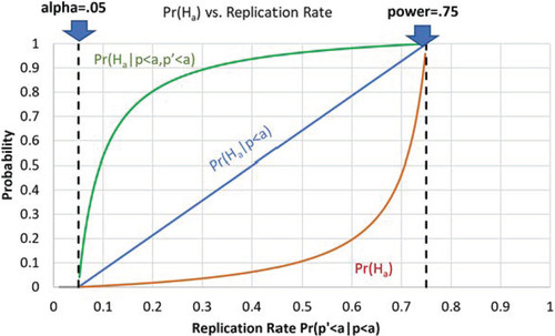
Figure 1 illustrates the relationship between the replication rate, the implied prior, α, and π. In the figure, we assume that $\alpha =0.05$ and $\pi =0.75$, and plot $\text{Pr}(H_a), \text{Pr}(H_a|P\le \alpha )$, and $\text{Pr}(H_a|P\le \alpha ,P\prime \le \alpha )$ in the bottom red curve, the middle blue line, and the top green curve, respectively, for different values of the replication rates in the field.

Fig. 1 Probability that the research proposition is true for different levels of replication in the field and number of significant results in independent studies. $\text{Pr}(H_a)$, $\text{Pr}(H_a|P\le \alpha )$, and $\text{Pr}(H_a|P\le \alpha ,P\prime \le \alpha )$ are shown in the bottom red curve, the middle blue line, and the top green curve, respectively.

As an illustration, suppose that in the field of adolescent depression, there was an attempt to reproduce 60 studies which initially had significant results where the power and significance level are consistently 0.8 and 0.05, respectively. Of these, 18 studies were found to have a statistically significant result using the same power and significance level. This gives us a reproduction rate of 0.3. Using Equation (1)(1) $$\text{Pr}\left(H_a\right)=\frac{\alpha (R-\alpha )}{{\pi }^2-{\alpha }^2+R(\alpha -\pi )}.$$(1) , we can compute that the prior probability now for any proposed study in the field is estimated to be$$\text{Pr}\left(H_a\right)=\frac{0.05\times (0.3-0.05)}{{0.8}^2-{0.05}^2+0.3\times (0.05-0.8)}=0.0303.$$

Then, lacking any other information about a proposed study other than these stated parameters describing the field of research from which the study is drawn, we would say the hypothesis has a 0.0303 probability of being true. If the study then produces a statistically significant result, we could apply equation (2)(2) $$\text{Pr}\left(H_a\right|P<\alpha )=\frac{(R-\alpha )}{(\pi -\alpha )}.$$(2) above and conclude that the tested hypothesis only has a one-in-three chance of being true$$\text{Pr}\left(H_a\right|P<\alpha )=\frac{0.3-0.05}{0.8-0.05}=0.333.$$

Does $\text{Pr}(H_a|P\le \alpha )=0.333$ seem low? It should be low with such a low rate of reproducible studies. Remember we stated the reproduction rate of studies—which were initially found to have statistically significant results—was only 18 out of 60. If every hypothesis being proposed was false, then we would still find that the reproduction rate approaches α after a large number of reproduction studies have been conducted. If every hypothesis were true, then the rate of reproduction would approach the power in the long run. (Of course, in practice it may not be the case that $\alpha <R<\pi$ if the number of studies is not large.) See the Appendix to confirm this result.

Finally, when and if those results are reproduced using the same alpha and power, we can again update the probability to be 0.889 using Equation (3)(3) $$\text{Pr}\left(H_a\right|P\le \alpha ,P\prime \le \alpha )=\frac{{\pi }^2 \text{Pr}\left(H_a\right)}{{\pi }^2 \text{Pr}\left(H_a\right)+{\alpha }^2(1- \text{Pr}(H_a\left)\right)}.$$(3) $$\begin{array}{c} \text{Pr}\left(H_a\right|P<\alpha ,P<\alpha )\\ \hspace{1em}\hspace{1em}=\frac{{0.8}^2\times 0.0303}{{0.8}^2\times 0.0303+{0.05}^2\times (1-0.0303)}=0.889.\end{array}$$

Most importantly, this approach allows us to simply abandon the use of significance tests altogether once we compute $\text{Pr}(H_a)$ from the previous reproduction studies. We can update $\text{Pr}(H_a)$ with a set of observations by using a BF $\text{Pr}( \text{data}|H_a)/ \text{Pr}( \text{data}|H_0$) and update it in a similar fashion again when this study is reproduced. The proposed equations need only be a way of computing a starting point for priors in a given field of research.

6 “Statistically Significant” May Still Only Mean “Slightly More Likely Than Not to Be False”

Suppose that a replication study was done similar to the Open Science Collaboration project, where 36 out of 100 studies were successfully reproduced, and where power was 0.75 for both the original research and its replication, and α was set at 0.05 for both in all initial studies and replication studies.

Note that we can and should treat the estimate of the replication rate R as itself being estimated from a population. This would be done with a beta distribution on R. We recommend naïve priors for this, such as Beta(1/2,1/2), the Jeffreys prior for R. For the estimate of $\text{Pr}(H_a)$ for a single proposition, we only need the mean of the beta distribution which, with the Jeffreys prior, would be $(a+1/2)/(a+b+1)$ where a is the number of successful replications in a field and b is the number of replications which were attempted but were unsuccessful. The prior will make a larger difference in a field when few replication studies have been attempted. Using the observed replications to compute the mean of an estimate of a population proportion of successful replication, this would produce an $R=(36+0.5)/(100+1)=0.361$. In this case, the number of replications is large enough that the Jeffreys priors have only a small impact on the estimated replication rate.

This replication rate would produce estimates of $\text{Pr}(H_a)=0.05$ and $\text{Pr}(H_a|P\le \alpha )=0.44$. This is roughly in agreement with findings by Berger and Sellke (1987) where they demonstrated that $\text{Pr}(H_0|P\le 0.05)=0.52$ for n = 50, which results in $\text{Pr}(H_a|P\le \alpha )=0.48$. If these findings hold for other fields then, based on conventional significance tests, we should expect to see that the probability of a proposition being true given a “significant” result is on the order of a coin flip. This alone may leave researchers—as well as news media and other users—with the sense that more needs to be done before making a confident declaration about a new finding.

Note that an important feature of this method is that publication bias, p-hacking or even outright fraud of the original study does not affect these calculations, as long as the reproduction study is conducted independently of the original study. If such factors are common in a field, then naturally the replication rate will be lower. Furthermore, once we establish this prior for a population of research studies, $\text{Pr}(H_a|P\le \alpha )$ can be updated using the updating property of Bayes’ theorem.

7 Level 2 Priors: A Conceptual Overview

Level 2 priors are informed priors that allow for discrimination among different propositions. Recall that Level 0 and (the strongly preferred) Level 1 both only provide priors for a randomly selected proposition out of a population of potential propositions. They do not differentiate among propositions based on their individual characteristics. In Level 1, we do not take into account any knowledge about the proposition that may differentiate it from others in the field. However, in Level 2 priors we utilize characteristics of individual studies to differentiate among them. Level 2 could be much more involved than Level 1 but our goal here is to review the potential benefits of more advanced analytics for statistical inference.

One example of a property that may differentiate an informed prior on a study from other studies in a field is who sponsors the study. Research has shown that the sponsor of the research may have bearing on outcomes. Rochon et al. (1994) and Friedberg et al. (1999) are two early references that show that studies sponsored by drug companies are much more likely to result in favorable results for the new drug than studies funded by not-for-profit organizations. The replication rates would just be estimated separately for different sponsors of research. This could also be done for considerations such as whether the study was properly registered (indicating a lower potential for publication bias) and previous retractions of a research institute. Equivalently, the field-level prior could be adjusted using study-level information to improve the estimation of $\text{Pr}(H_a|P\le \alpha )$ in a specific study.

Another way to tailor these implied, informed priors to specific propositions is to rely on the judgment of reviewers, who are experts in the field. It may be beneficial to involve reviewers earlier in the research process, so that they can provide input at the time when the study is registered but has not yet been conducted. These reviews could involve subjective adjustments to the previously objectively computed priors. This would allow the prior to be informed on characteristics of the proposed research other than what was explicitly parametrized, such as how well the hypothesis supports or contradicts previously known principles in the field.

There is ample evidence that reviewers could be made to be well calibrated in these estimates. The literature on calibration of subjective probabilities defines well-calibrated as a process that produces probabilities that, in subsequent observations, closely matches observed frequencies. That is, when an individual (e.g., a weather forecaster) applies a large number of subjective probabilities to events (rain the following day), it is determined that of all the times when the individual said something had a probability of 0.2, it was observed to occur 20% of the time. Likewise, events occur at a rate of 10% when they say the probability is 0.1, and so on (Murphy and Winkler 1977; Lichteinstein 1981; Ungar et al. 2012). Studies have shown that individuals do not initially perform well in such tasks. They may be extremely overconfident that the observed frequency of an event is much lower than the stated probability and in some contexts may be under-confident. Yet it has also been shown that it is possible to almost eliminate either bias using some combination of training, elicitation techniques, incentives, aggregation, and mathematical transformations of the estimates. These methods are referred to as calibrating or de-biasing the subjective probabilities (Ferrell and Goey 1980; Fellner and Krüger 2012). A related body of literature addresses the question of elicitation of information from experts. Brownstein et al. (2019) discuss the critical role of expert judgment in the various steps in the scientific process and in decision making, and conclude that establishing reliable protocols for obtaining input from experts is important. O’Hagan (2019) agrees and argues that subjective judgment is inevitable in scientific inference and decision making. He adds that the fact that expert judgment is subjective does not mean that it cannot be elicited in a scientifically valid way, so that the chance of bias is minimized.

At this point, however, we are only recommending that the data about reviewer estimates at least begin to be recorded. How those estimates could subsequently be used to improve the performance of the prior estimation process should be a subject of further study, along with other data analysis about sponsors and other objective characteristics. But at least that field of research would have the data to start evaluating alternative methods. It would be ironic, in fact, if a field like psychology objected to at least evaluating the approach we propose.

8 Quality Control for Science

A feature of both Level 1 and 2 priors is the potential for greatly improved responsiveness. Again, by responsiveness, we mean the ability of researchers in a field to detect and respond to problems in their field in a more timely manner instead of decades of delay. Level 0 creates a naïve prior for an entire field and, like the traditionally recommended significance levels, does not change as replication rates are updated. Levels 1 and 2, however, offer the basis for more frequently evaluated performance of a field. We can purposely collect and record the metadata resulting from the process of conducting research. By metadata, we refer to attributes of the publication process rather than the content of the publication itself, the type of information about submissions that journals and professional societies currently do not track. This allows for a type of “quality control” for science.

At the level of the study itself, information to be recorded might include effect size, p-value, reputation of investigator, source of funding for the work, degree of “surprise” associated with claim(s), sample size, and many others. At the level of the field itself, we could record the number of retractions in the field, the proportion of studies that get reproduced successfully, and such. Finally we could also keep track of attributes associated with the journal in which a study appeared, and that might include the impact factor for the journal, its acceptance rate, number of volumes, pages per year, etc.

In principle, as more metadata become available, we could think of deploying the type of tools that are used in other fields to classify items into two or more categories. In our case, the “item” is a research claim, and the categories might be “true” and “false.” It is standard to train classification algorithms using a large set of items for which we know “ground truth,” that is, a large number of research claims for which we “know” whether they are really true or false. These algorithms, generally known as supervised learning algorithms (e.g., Breiman 2001) “learn” which combinations of the various meta-variables are typically observed when two items belong in the same category or in a different category. The output is a score, or an empirical probability of membership in each of the two classes.

In the research enterprise, we do not typically get to observe ground truth, as we do not know which proposition is true and which is false. But as described in Section 4, we can estimate the probability that a claim is true, and agree on a convention that says that for the purpose of training a classifier, we will declare that any claim with a probability of occurrence above say 0.75 is “true.” Given a large number of “true” and “false” claims and the corresponding metadata, we could compute the empirical class probability for each item in each class, and then construct (and periodically update) a distribution of classification score for “true” and for “false” claims. With the same algorithm, a potential user of a specific research paper would then proceed as follows:

• First, compute the corresponding score, or empirical probability that the claim is true using the classification algorithm.

• Next, compare the empirical probability to the distribution of scores obtained for “true” claims and the distribution of scores obtained from the “false” claims.

The user can then decide whether her score is more typical if the claim is “true” than if the claim is “false.”

For illustration, we use the following simple example. In a specific field, investigators attempted to reproduce 200 studies, and in 100 of those studies, the results were the same as those obtained by the initial researchers. In the other 100, the reproduced study failed to reach the same conclusion. Suppose that for each of the 200 original studies we have information on metadata including the source of funding for the study, the number of retractions associated with the investigator, the sample size and whether the investigator had “registered” the study or not. A logistic regression model with a binary response (Y = 1 if results were reproduced, and Y = 0 otherwise) and with the meta-variables as predictors in the model can be fit using the 200 studies. If a new paper is published that concludes H_a in some problem, we can evaluate the logistic regression model using the metadata for the new study, and compute an empirical probability that the results will reproduce if the study is repeated. If, from the training studies, we know that when results reproduce, the empirical probabilities vary between 0.6 and 0.99, and when results do not reproduce, the range of empirical probabilities is between 0.0 and 0.45, then this provides information that we can use to predict whether the new study’s claim is or is not likely to hold should the study be reproduced.

In the ideal scenario (and in the simple example above), the strength of the score we compute for a proposition would correspond closely with the probability that the proposition is true, computed as described earlier. Here, the classifier plays the role of the expert in that it combines many different pieces of information in some optimal way to produce the best (in some sense) assessment of $\text{Pr}(H_a)$. The effectiveness of the data-science approach we discuss is critically dependent on the information that is used to train the classifier, so at this time we present it more as an idea for the future than as something that can be implemented soon.

9 Conclusions

We propose that the generation of priors for a field of research is both feasible and necessary. We have argued that uninformed priors are as objective as significance levels if objective is taken to mean “impartial” or in the sense that a calculation is objective when it assumptions are explicit. We also know that, unlike significance levels, priors are necessary to compute the probability that a proposition is true given the data and the assignment of probabilities to outcomes is necessary for decisions under uncertainty. This addresses the issue of relevance.

We also show how such priors could be computed from reproduction studies even though the reproduction studies themselves rely on conventional significance tests and do not directly compute the probability that a proposition is true. Also, using examples from existing research, we show that the probability that a hypothesis is true after the initial positive finding will often be somewhere in the range of a coin flip (0.5) or lower.

We believe that explicitly publishing such a probability in the abstract of a paper will make users, media, and other researchers more likely to see the finding as tentative instead of final. This may either encourage further reproduction itself or even encourage the original researchers to increase the sensitivity of a study so that the initial finding produces a probability of greater than 0.95 or 0.99.

Priors may be further improved by using information that discriminates among different proposals (as opposed to estimating a single prior for a random proposition out of a population of potential propositions). Using metadata about the performance of studies as described earlier (e.g., reproduction rates, sponsors, reviewer estimates, etc.), would allow for different priors for propositions of different types. Further differentiation may be made by utilizing subjective estimates of reviewers once sufficient data has been collected on estimates from reviewers and a de-biasing/calibration method has been determined which best predicts results of original studies and reproduction studies.

Finally, consistently updating priors for all studies in a field based on reproduction results is one way to address the issue of responsiveness. This creates a process of continuous statistical quality control for science similar to what is done in real-time manufacturing environments. Reproductions, retractions, reviews and more can be tracked and used to update priors (Barlow and Irony 1992; Deming 2000). In these methods, often known as statistical process control, when any one of these metrics meets a “control limit” a specific intervention action would be required. Instead of waiting years or even decades to detect a problem, potential issues are monitored with each publication, reproduction, or retraction. If responsiveness is not improved, reproduction can only continue to improve at a snail’s pace, if at all.

We are certainly not the first authors to address these types of issues, but we do offer a different perspective from what has been published in the literature. In addition to publications that have already been referenced in this work, we highlight the work of Sellke et al. (2001), Nuzzo (2014), and Fraser (2017). Sellke et al. (2001) were early critics of science’s reliance on p-values for decision making, and proposed an approach to calibrate p-values so that those calibrated p-values better correspond to the $\text{Pr}(H_a| \text{data})$. Nuzzo discussed the key role of $\text{Pr}(H_a| \text{data})$ in the decision making process, but she did not elaborate on how to implement a process to get to the desired outcome. Finally, Fraser (2017) demonstrates that p-values can be the bases for a complete inferential framework, and highlights the notion that the fact that p-values have been mis-used and even abused, this does not subtract from their worth as indicators of the distance between the data and a parameter value.

To conclude, we recommend that an entity (e.g., the journal, professional association, university, or other agency) be identified to implement and manage the following:

1. A field should implement the research registries, data sharing, and other standards recommended by the Manifesto.

2. Implementing Level 1 priors can begin in parallel with 1) above. Jeffreys prior for reproduction rates would be updated with reproduction studies from that field. Methods for generalizing this approach to the broader question of effect sizes will need to be developed. More precisely,

   1. A journal, professional association or other entity should implement, at a minimum, a Level 0 prior or, preferably skip directly to a Level 1 prior if there are adequate reproductions.

   2. If reproductions in a given field of research are too few, too old, or nonexistent, then that field should immediately organize reproduction studies to bootstrap the informed implied prior of Level 1.

   3. Published research should clearly disclose the updated priors and posterior probabilities of a proposition in the abstract or directly under the authors’ names. In an online source, these probabilities would be updated dynamically with new reproduction studies.

3. A plan for implementing Level 2 priors should be specified including the following:

   1. Parameters of studies which could be used to discriminate priors among different propositions can be investigated. Where such candidate parameters have sufficient predictive utility, then they can be incorporated as part of a prior estimation and continuous quality control.

   2. A research field should change the peer review process so that reviewers are shown proposed research before it is completed. Those reviewers should be asked to estimate subjective probabilities for proposed research including the probability of a positive result and the probability that reproduction, if attempted, will support the earlier study. As these data are gathered, training, transformations and other calibration methods can be tested. If such a method is found to be well-calibrated, then subjective probabilities of reviewers can be incorporated into the estimate of priors.

   3. Decision criteria for interventions may be established by identifying control limits for each of the tracked metrics. Corrective interventions in a field may include changing the recommended power of studies, research methods, or how they are reviewed.

   4. More advanced data analytic methods can be used (and, of course, monitored for performance) to further improve reproduction, relevance and responsiveness.

In summary, the reproducibility crisis is best handled when managed in concert with relevance and responsiveness. We believe that our recommendations are feasible, reasonable, flexible and ultimately necessary, and that beginning the discussion on how to best implement the approach we propose can be accomplished.

Additional information

Funding

Alicia L. Carriquiry gratefully acknowledges partial support from the Center for Statistics and Applications in Forensic Evidence (CSAFE) through Cooperative Agreement #70NANB15H176 between NIST and Iowa State University, which includes activities carried out at Carnegie Mellon University, University of California Irvine, and University of Virginia.

Appendix

Recall from the notation in Section 6 that the Type I error α is defined as the probability of incorrectly concluding H_a, or $\text{Pr}(P\le \alpha |H_0)$. Given the null hypothesis and if the original and the reproduction studies have the same α and are statistically independent, the probability that both studies will exhibit significant results is$$\text{Pr}(P\le \alpha |H_0) \text{Pr}(P\prime \le \alpha \left|H_0\right)$$or simply ${\alpha }^2$. Similarly, if H_a is true, then the probability that both studies would produce significant results is ${\pi }^2$, assuming that the Type II error β was the same in both studies.

Now, using the law of total probability, we can write(4) $$\begin{array}{c} \text{Pr}(P\le \alpha )= \text{Pr}(P\le \alpha |H_a) \text{Pr}(H_a)+ \text{Pr}(P\le \alpha \left|H_0\right)[1- \text{Pr}(H_a\left)\right]\\ =\pi \text{Pr}\left(H_a\right)+\alpha [1- \text{Pr}(H_a\left)\right].\end{array}$$(4)

By the same line of reasoning, we have that(5) $$\begin{array}{c} \text{Pr}(P\le \alpha ,P\prime \le \alpha )= \text{Pr}(P\le \alpha ,P\prime \le \alpha |H_a) \text{Pr}(H_a)\\ + \text{Pr}(P\le \alpha ,P\prime \le \alpha |H_0\left)\right[1- \text{Pr}\left(H_a\right)]\\ ={\pi }^2 \text{Pr}\left(H_a\right)+{\alpha }^2[1- \text{Pr}(H_a\left)\right].\end{array}$$(5)

Using the equality in (4) and letting $R= \text{Pr}(P\prime \le \alpha |P\le \alpha )$ denote the reproduction rate, we find that$$R\{\pi \text{Pr}(H_a)+\alpha [1- \text{Pr}\left(H_a\right)\left]\right\}={\pi }^2 \text{Pr}\left(H_a\right)+{\alpha }^2[1- \text{Pr}(H_a\left)\right],$$

so that after some rearrangement we can solve for $\text{Pr}(H_a)$ to get(6) $$\text{Pr}\left(H_a\right)=\frac{\alpha (R-\alpha )}{{\pi }^2-{\alpha }^2+R(\alpha -\pi )}.$$(6)

The prior $\text{Pr}(H_a)$ we just obtained in (6) can now be used to estimate the probability that the proposition in the first study was true, given that the investigators rejected H₀ as follows(7) $$\begin{array}{c} \text{Pr}\left(H_a\right|P\le \alpha )=\frac{ \text{Pr}\left(H_a\right) \text{Pr}(P\le \alpha |H_a)}{ \text{Pr}\left(H_a\right) \text{Pr}(P\le \alpha |H_a)+[1- \text{Pr}\left(H_a\right)] \text{Pr}(P\le \alpha \left|H_0\right)}\\ =\frac{\pi \text{Pr}\left(H_a\right)}{\pi \text{Pr}\left(H_a\right)+\alpha [1- \text{Pr}(H_a\left)\right]}.\end{array}$$(7)

It follows from all of the above that(8) $$\text{Pr}\left(H_a\right|P\le \alpha ,P\prime \le \alpha )=\frac{{\pi }^2 \text{Pr}\left(H_a\right)}{{\pi }^2 \text{Pr}\left(H_a\right)+{\alpha }^2[1- \text{Pr}(H_a\left)\right]}.$$(8)

The linearity of $\text{Pr}(H_a|P\le \alpha )$ shown in Figure 1 may be surprising, but when it is simplified it becomes more obvious. Substitute the $\text{Pr}(H_a)$ in the function for $\text{Pr}(H_a|P\le \alpha )$ in (7). Then multiply the numerator and denominator of by $(R-\alpha )/ \text{Pr}(\mathit{Ha})\pi$ and expand the expressions. We would find that a number of terms cancel each other out and we are left with$$\text{Pr}\left(H_a\right|P<\alpha )=\frac{(R-\alpha )}{(\pi -\alpha )}.$$

Notes

1 We recognize the debate about the use of “reproduction” versus “replication” in this context. We will use the former term unless we refer to the work of earlier authors who used the latter. In that case, we will use their terminology to avoid confusion.

2 Like any definition of a population, what constitutes a field will inevitably be somewhat arbitrary. (However, researchers refer to their “fields” usually without need for further clarification, especially when speaking to others they see as peers in their “field.”)

References

- Barlow, R. E., and Irony, T. Z. (1992), “Foundations of Statistical Quality Control,” in Current Issues in Statistics: Essays in Honor of D. Basu, Lecture Notes—Monograph Series (Vol. 17), New York: Springer.
- Berger, J. O., and Sellke, T. (1987), “Testing Point-Null Hypotheses: The Irreconcilability of p-Values and Evidence,” Journal of the American Medical Association, 82, 112–122. DOI: 10.2307/2289131.
- Breiman, L. (2001), “Random Forests,” Machine Learning, 45, 5–32. DOI: 10.1023/A:1010933404324.
- Brownstein, N., Louis, T., O’Hagan, A., and Pendergast, J. (2019), “The Role of Expert Judgment in Statistical Inference and Evidence-Based Decision Making,” The American Statistician.
- Buckheit, J. B., and Donoho, D. L. (1995), “WaveLab and Reproducible Research,” Technical Report #474, Department of Statistics, Stanford University, Stanford.
- Casadevall, A., and Fang, F. C. (2010), “Reproducible Science,” Infection and Immunity, 78, 4972–4975. DOI: 10.1128/IAI.00908-10.
- Deming, W. E. (2000), Out of the Crisis (1st ed.), Cambridge, MA: MIT Press.
- Dickersin, K. (1990), “The Existence of Publication Bias and Risk Factors for Its Occurrence,” Journal of the American Medical Association, 263, 1385–1389. DOI: 10.1001/jama.1990.03440100097014.
- Fellner, G., and Krüger, S. (2012), “Judgmental Overconfidence: Three Measures, One Bias?,” Journal of Economic Psychology, 33, 142–154. DOI: 10.1016/j.joep.2011.07.008.
- Ferrell, W. R., and Goey, P. J. (1980), “A Model of Calibration of Personal Probabilities,” Organizational Behavior and Human Decision Processes, 26, 32–56. DOI: 10.1016/0030-5073(80)90045-8.
- Fisher, R. A. (1973), The Design of Experiments (9th ed.), New York: MacMillan.
- Fraser, D. A. S. (2017), “p-Values: The Insight to Model Statistical Inference,” Annual Reviews in Statistics and its Applications, 4, 1–14. DOI: 10.1146/annurev-statistics-060116-054139.
- Friedberg, M., Saffran, B., Stinson, T. J., Nelson, W., and Bennett, C. L. (1999), “Evaluation of Conflict of Interest in Economic Analyses of New Drugs Used in Oncology,” Journal of the American Medical Association, 282, 1453–1957. DOI: 10.1001/jama.282.15.1453.
- Goodman, S. N. (1999), “Toward Evidence-Based Medical Statistics: 1. The p-Value Fallacy,” Annals of Internal Medicine, 130, 995–1004. DOI: 10.7326/0003-4819-130-12-199906150-00008.
- Howard, R. A., and Abbas, A. E. (2015), Foundations of Decision Analysis (1st ed.), New York: Pearson.
- Howard, R. A., and Matheson, J. E. (1977), Readings in Decision Analysis, Menlo Park, CA: SRI International.
- Howard, R. A., and Matheson, J. E. (1984), Readings on the Principles and Applications of Decision Analysis (2 vols.), Menlo Park, CA: Strategic Decisions Group.
- Hubbard, R. (2016), Corrupt Research: The Case for Re-conceptualizing Empirical Management and Social Science (1st ed.), Los Angeles, CA: Sage.
- Ioannidis, J. P. (2005), “Why Most Published Research Findings Are False,” PLoS Medicine, 2, e124, DOI: 10.1371/journal.pmed.0020124.
- Jager, L. R., and Leek, J. T. (2014), “An Estimate of the Science-Wise False Discovery Rate and Application to the Top Medical Literature,” Biostatistics, 15, 1–12. DOI: 10.1093/biostatistics/kxt007.
- Jaynes, E. T. (1958), “Prior Probabilities,” IEEE Transactions on Systems Science and Cybernetics, 4, 227–241. DOI: 10.1109/TSSC.1968.300117.
- Jaynes, E. T. (2003), Probability Theory: The Logic of Science, London: Cambridge University Press.
- Kerr, N. L. (1998), “HARKing: Hypothesizing After the Results are Known,” Personality and Social Psychology Review, 2, 196–217. DOI: 10.1207/s15327957pspr0203_4.
- Lichteinstein, S., Fischhoff, B., and Phillips, L. (1981), Calibration of Probabilities: The State of the Art to 1980. Technical Report PTR-1092-81-6 to Offfice of Naval Research, Contract No. NOOO14-80-C-0150.
- Munafò, M. R., Nosek, B., Bishop, D. V. M., Button, K. S., Chambers, C. D., Percie du Sert, N., Simonsohn, U.,Wagenmakers, E.-J., Ware, J. J, and Ioannidis, J. P. (2017), “A Manifesto for Reproducible Science,” Nature Human Behavior, 1, 0021. DOI: 10.1038/s41562-016-0021.
- Murphy, A. H., and Winkler, R. L. (1977), “Reliability of subjective Probability Forecasts of Precipitation and Temperature,” Journal of the Royal Statistical Society, Series C, 26, 41–47. DOI: 10.2307/2346866.
- Nuzzo, R. (2014), “Scientific Method: Statistical Errors,” Nature, 506, 150–152. DOI: 10.1038/506150a.
- O’Hagan, A. (2019), “Expert Knowledge Elicitation: Subjective But Scientific,” The American Statistician.
- Open Science Collaboration (2015), “Estimating the Reproducibility of Psychological Science,” Science, 349, aac4716.
- Popper, K. (1959), The Logic of Scientific Discovery, London: Routledge.
- Rochon, P. A., Gurwitz, J. H., Simms, R. W., Fortin, P. R., Felson, D. T., Minaker, K. L., and Chalmers, T. C. (1994), “A Study of Manufacturer Supported Trials of Non-steroidal Anti-inflammatory Drugs in the Treatment of Arthritis,” Archives of Internal Medicine, 154, 157–163. DOI: 10.1001/archinte.1994.00420020059007.
- Rosenthal, R. (1979), “The File Drawer Problems and Tolerance for Null Results,” Psychological Bulletin, 86, 638–641. DOI: 10.1037/0033-2909.86.3.638.
- Sackett, D. L. (1979), “Bias in Analytic Research,” Journal of Chronic Diseases, 32, 51–63.
- Savage, L. J. (1954), The Foundations of Statistics, New York: Wiley.
- Sellke, T., Bayarri, M. J., and Berger, J. O. (2001), “Calibration of p-Values for Testing Precise Null Hypothesis,” The American Statistician, 55, 62–71. DOI: 10.1198/000313001300339950.
- Sterling, T. (1959), “Publication Decisions and Their Possible Effects on Inferences Drawn From Tests of Significance,” Journal of the American Statistical Association, 54, 30–34. DOI: 10.2307/2282137.
- Stodden, V. (2015), “Reproducing Statistical Results,” Annual Reviews of Statistics and its Application, 2, 1–19. DOI: 10.1146/annurev-statistics-010814-020127.
- Stodden V., Guo, P., and Ma, Z. (2013), “Toward Reproducible Computational Research: An Empirical Analysis of Data and Code Policy Adoption by Journals,” PLoS One, 8, e6711.
- Ungar, L., Mellors, B., Satopää, V., Baron, J., Tetlock, P., Ramos, J., and Swift, S. (2012), “The Good Judgment Project: A Large Scale Test of Different Methods of Combining Expert Predictions,” AAAI Technical Report FS-12-06, Association for the Advancement of Artificial Intelligence, University of Pennsylvania.
- Von Neumann, J., and Morgenstern, O. (1944), The Theory of Games and Economic Behavior, Princeton, NJ: Princeton University Press.
- Wald, A. (1950), Statistical Decision Functions, New York: Wiley.