Hidden Markov Models for Low-Frequency Earthquake Recurrence

Abstract

Low-frequency earthquakes (LFEs) are small magnitude earthquakes with frequencies of 1–10 Hertz which often occur in overlapping sequence forming persistent seismic tremors. They provide insights into large earthquake processes along plate boundaries. LFEs occur stochastically in time, often forming temporally recurring clusters. The occurrence times are typically modeled using point processes and their intensity functions. We demonstrate how to use hidden Markov models coupled with visualization techniques to model inter-arrival times directly, classify LFE occurrence patterns along the San Andreas Fault, and perform model selection. We highlight two subsystems of LFE activity corresponding to periods of alternating episodic and quiescent behavior.

Keywords:

• Classification
• Model selection
• San Andreas fault
• Visualization
• Viterbi path

1 Introduction

Low-frequency earthquakes (LFEs) are brief slip events that are triggered adjacent to major faults with frequencies of between 1 and 10 Hertz (Shelly 2017). They typically occur in overlapping sequence forming seismic tremors (Supino et al. 2020). Seismic tremors are associated with the occurrence of slow slip events in the phenomenon of episodic tremor and slip (e.g., Rogers and Dragert 2003; Peterson and Christensen 2009; Obara 2011). Slow slip events are fault movements that occur on longer timescales, over days or even years. These have been linked to megathrust earthquakes through their seismogenic location and slip mechanisms, and studying their behaviors has the potential to improve the forecast of large earthquakes (Obara and Kato 2016). However, the nature of slow slip makes it often hard to identify geodetically. Tremors and their decomposed events LFEs are easier to detect and extensive recording networks are able to provide a good catalog of these events (e.g., Shelly 2017). Therefore, LFE analysis is crucially important in facilitating the collection of slow slip data, and supports further understanding of the relationship between slow slip events and large earthquakes.

There is a comprehensive catalog of LFE occurrence data along the San Andreas Fault, recorded since 2001 and made available by Shelly (2017). Some slow slip activity has been detected from Global Navigation System data (e.g., Rousset, Bürgmann, and Campillo 2019; Michel et al. 2022) which confirms the occurrence of episodic tremor and slip here, but the existing slip data are far from complete. Characterizing the temporal changes in LFE recurrence provides insights into the evolution of generating mechanisms that give rise to episodic tremor and slip and will strengthen methods for the detection and modeling of slow slip events.

To date, there has been no systematic statistical analysis carried out on LFEs to study in detail their occurrence patterns and hence infer their generation processes. This analysis will focus on the specific characteristics of recurrence patterns within a San Andreas LFE family. Earthquake data are typically modeled as point processes (e.g., Ogata 1988; Bebbington and Harte 2003; Bray and Schoenberg 2013; Ho and Bhaduri 2015; Ignatieva, Bell, and Worton 2018; Shcherbakov et al. 2019). Based on Shelly (2017), LFEs occur randomly in time, and could occur in clusters which recur in time. Point processes with recurring temporal patterns, where different patterns consist of different rates of event occurrence, can be considered as point processes with change points. When change points occur frequently and similar occurrence patterns recur between multiple change points, a Markov-modulated point process is typically used, such as Markov-modulated Poisson processes or Markov-modulated Hawkes processes (e.g., Lu 2012; Wang, Bebbington, and Harte 2012). These models allow the point process to be dependent on a continuous-time Markov chain, each state of which represents a distinct event generation mechanism. However, such models often involve complicated mathematical derivation and expensive computational cost (Wang, Bebbington, and Harte 2012; Wang, Wang, and Zhuang 2018). Developing a Markov-modulated renewal process and its estimation method is not a trivial task, and the results are challenging to interpret.

A point process can be equivalently represented by its occurrence times, inter-arrival times and counting process N(t). The typical procedure in point process literature involves modeling the occurrence times and estimating the intensity function (instantaneous rate of occurrence), with the continuous-time Markov chain modulated point processes being based on this. In this manuscript, we propose a simpler way to model point processes with numerous change points and recurring temporal patterns. We propose to model the inter-arrival times of LFEs directly using discrete-time hidden Markov models (HMMs) to describe continuous-time point processes. The discrete-time hidden Markov chain captures the recurring temporal patterns and finds the change points. We then propose some post model-fitting analysis to extract important practical information from the model results, and hence reveal the inner workings of the system and provide useful interpretations of the findings. HMMs simplify the inference procedure while providing the same effective output. This idea can be implemented for more complicated point processes across applications. For example, while not necessary to describe the mechanisms of LFEs, self-exciting point processes would be effectively modeled using HMMs as each time point is dependent on the immediately previous event.

HMMs have wide applications, examples include spike data from neural circuits (e.g., Tokdar et al. 2009; Escola et al. 2011), seismic and volcanic activity (e.g., Bebbington 2007; Wang and Bebbington 2012; Bhaduri 2020), and ecological studies (e.g., Borchers and Langrock 2015; McClintock et al. 2020). Wang et al. (2017, 2018) have highlighted the usefulness of HMMs for understanding seismogenic activity. A special type of HMMs was developed to model the spatial locations of seismic tremors, finding a considerable improvement on previous manual classification (Buckby et al. 2020). As tremors and LFEs are governed by the same underlying geological processes, this motivates the use of HMMs for effective classification of LFE observations.

We will examine the specific characteristics of recurrence patterns within one LFE family along the San Andreas Fault. LFE families are spatially localized patches of repeating LFEs (van der Elst et al. 2016). The spatial scale on which individual LFEs vary is small and it is not possible to accurately locate specific events, thus all events within a LFE family are assigned to the same centroid location (latitude, longitude and depth). The convention when analyzing LFE events along the San Andreas is to consider behavior within these defined families (e.g., Wu et al. 2013, 2015; Veedu and Barbot 2016; Thomas et al. 2018).

Past research using HMMs to analyze point process data such as earthquakes or volcanic eruptions typically stops at classification or a simple forecast of future activity. Point process data are often generated by complex systems and it is important to understand as much about the underlying processes as possible. This article will demonstrate the wealth of additional information that can be uncovered from the fitting results of HMMs by carrying out post-fitting analysis and using graphical techniques to display, understand, and communicate findings. We will also explore the use of these techniques to aid model selection, an enduring problem for HMMs (Buckby 2020). The methods introduced in this article can be readily used in a wide range of applications of HMMs.

Section 2 introduces the LFE data, and the motivation of using HMMs. Section 3 describes the components of HMMs, the optimization process, model selection criteria, and post-fitting analysis. Section 4 provides results and graphical aids for model selection, checking, and interpretation of the fitted HMMs applied to LFE data. Section 5 concludes the article and explores future research directions.

2 Data

The San Andreas LFE data was compiled by Shelly (2017) from recordings collected by a High-Resolution Seismic Network (HRSN) along 150km of the central fault. Events occurred at depths of between ∼16km and 30km, from the lower crustal to upper mantle areas. The original catalog contains data from the April 6, 2001 to the September 19, 2016. This includes some periods when the network was operating only at partial capacity or completely offline, and others when it was affected by high noise levels (Shelly 2017). These issues are largely concentrated at the beginning of the catalog, with a notable increase in the number of events detected from November 2003. In order to reduce the effect of missing events our analysis will use the observations since January 1, 2004, a period which includes the occurrence of the notable magnitude 6 Parkfield earthquake on the 28th of September 2004.

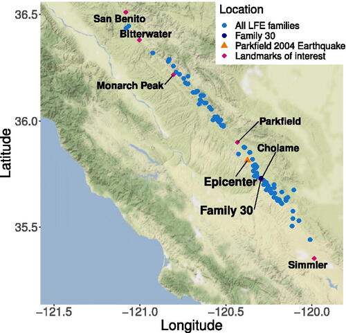
LFEs provided in the Shelly (2017) catalog were detected using waveform templates created by Shelly and Hardebeck (2010), and assigned to one of 88 families according to highest summed correlation coefficient. Latitude, longitude, and depth location are specified by family rather than individual observation, due to the level of uncertainty at this scale. The centroid locations for each family can be seen in Figure 1. These represent all LFE detections nearest to that location and therefore assigned to that family.

Fig. 1 Map of the San Andreas Fault with the locations of LFE families indicated (note the location of family 30 overlaps the town of Cholame). Created using ggmap with the RStudio api (Kahle and Wickham 2013; Ushey et al. 2020).

Event times were recorded in seconds and converted to Julian day equivalents with origin January 1, 2004. Patterns of LFE occurrence may be broadly categorized as either episodic or continuous. LFE generating zones that exhibit substantial periods of activity alternating with inactivity are defined as episodic. Other families of LFEs display a consistent, continuous activity rate. Patterns of LFE recurrence can also change over time or be affected by other fault events (Shelly and Johnson 2011). Less episodic, that is, more continuous, behavior is associated with increases in activity. Changes in the level of LFE activity may be due to event recurrence rate affecting fault friction, friction referring to the extent to which the fault is resistant to movement, or vice versa (Shelly 2017).

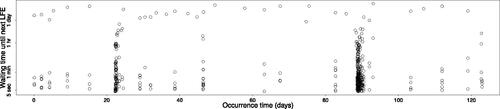
Let $Y_0,Y_1,\dots ,Y_n$ be the occurrence times of LFEs. The inter-arrival (waiting) times are defined as $X_t=Y_t-Y_{t-1}$, for $t=1,\dots ,n$. Inter-arrival time corresponds to the LFE activity rate. For example, shorter inter-arrival times indicate higher activity rate as events are occurring more frequently. Figure 2 presents the waiting times until the next event (i.e., inter-arrival times) versus the occurrence times for a subset of events observed in family 30 (ID 41767s). All events in this family were located to latitude ${35.73}^{°}$ N, longitude ${120.295}^{°}$W and depth 23.25km. The inter-arrival times are skewed so were log-transformed. This family displays episodic recurrence behavior, indicated by the high degree of temporal clustering of events. The two columns of many clustered points indicate episodic bursts, where sustained events are recorded over a short period of time. The background activity between these bursts is essentially quiescent, with small clusters alternating with long periods of inactivity. Family 30 is representative of episodic LFE activity in the area and thus our focus in this article.

Fig. 2 Inter-arrival times versus occurrence times of the first 500 events recorded from LFE family 30 (beginning January 1, 2004).

The dramatic variation in activity levels across time suggests that there is overdispersion (excess variation) present and these data should be modeled by mixture distributions. HMMs assume that these observed data come from several distinct distributions, each driven by a state of the unobserved generating processes. These are geological in nature, such as strain and friction variation due to the overarching tectonic stress.

Another important consideration is the serial dependence (correlation) displayed by the LFE activity. This is typical of earthquake data, as prior events generate changes in stress and plate structure that can have a direct causal effect on future activity. The dependence structure of the hidden Markov chain may be able to model this.

3 Methodology

HMMs are used to describe data where the observed values are generated by an underlying, unobserved process. The unobserved process is denoted $\{C_t:t=1,2,\dots \}$ and assumed to be a Markov chain satisfying the form of conditional dependence $\mathbb{P}(C_t|C_{t-1},\dots ,C_1)=\mathbb{P}(C_t|C_{t-1})$, where C_t is the state the chain is in at time t. Each hidden state C_t can take values from $i=1,\dots ,m$, which generate observed data with distinct features. We call the model an m-state HMM. The observed state-dependent process is denoted $\{X_t:t=1,2,\dots \}$ and the state-dependent distribution has probability density function (pdf) $f(x_t|x_1,\dots ,x_{t-1},C_1,\dots ,C_t)=f(x_t|C_t=i)=p_i(x)$.

3.1 Model Fitting

There are three components of an HMM to be estimated. The initial distribution of the Markov chain $\mathit{\delta }$ contains m probabilities ${\delta }_i=\mathbb{P}(C_1=i),i=1,\dots ,m$, satisfying $\sum _i{\delta }_i=1$. An m × m matrix $\mathbf{\Gamma }$ contains the transition probabilities between each pair of the hidden states, ${\gamma }_{ij}=\mathbb{P}(C_t=j|C_{t-1}=i)$, where $\sum _j{\gamma }_{ij}=1$. These are independent of t when the Markov chain is homogeneous. The third component is the set of parameters of each state-dependent distribution, defining the pdf $p_i(x)$. Given a sequence of observed data $x_1,\dots ,x_n$, the likelihood function of an HMM is given by $L_T=\mathit{\delta }\mathbf{\Gamma }\mathit{P}(x_1)\mathbf{\Gamma }\mathit{P}(x_2)\dots \mathbf{\Gamma }\mathit{P}(x_T)\mathbf{1}\prime$, where $\mathit{P}(x)$ is a diagonal matrix with the ith diagonal element $p_i(x)$.

Our analysis will consider homogeneous, stationary HMMs with a discrete state space. That is, we assume $\mathit{\delta }=\mathit{\delta }\mathbf{\Gamma }$. Likelihood maximization is carried out using iterative Nonlinear Minimization via a Newton-type algorithm with 1000 sets of initial values for each m-state model.

3.2 Model Comparison

The problem of order selection (deciding m) for HMMs is well recognized, with no consensus on a universally best criterion. Various criteria have been proposed and compared across simulation studies in a variety of contexts (e.g., Costa and De Angelis 2010; Bacci, Pandolfi, and Pennoni 2014; Holzmann and Schwaiger 2016; Pohle et al. 2017). Pohle et al. (2017) proposed a comprehensive set of steps for selecting an appropriate and meaningful HMM. However, these studies typically consider only a small number of true hidden states (frequently only 2 to 4) for sample sizes of 10,000 or often much less. The application of HMMs to tremor and LFE data requires selecting models fitted to observations of larger sample sizes, comparing a large number of hidden states to parsimoniously describe the complexity of the generating process.

Buckby (2020) compared a wide range of model selection criteria for HMMs with many states fitted to seismic tremor data, and provides a detailed examination of the benefits and drawbacks of potential selection criteria. If forecasting is the main goal of the analysis Akaike Information Criterion (AIC) generally has good performance. However, AIC has a tendency to overestimate the true number of states. When the focus is on classification Bayesian Information Criterion (BIC) is more useful, although BIC can underestimate the true number of states. The measures with the best performance struck a balance between these extremes. Buckby (2020) concluded that the Hannan-Quinn Information Criterion (HQC) (Hannan and Quinn 1979) and adjusted Bayesian Information Criterion (adjusted BIC) (Buckby 2020) were the most accurate among those criteria considered in selecting the true number of states. Let logL be the optimized log-likelihood, p be the number of model parameters, and n be the number of observed data points. The HQC is defined as $-2\hspace{0.17em}\log \hspace{0.17em}L+2p\hspace{0.17em}\log \hspace{0.17em}(\hspace{0.17em}\log \hspace{0.17em}(n))$, and the adjusted BIC is defined as $-2\hspace{0.17em}\log \hspace{0.17em}L+p\hspace{0.17em}\log \hspace{0.17em}(n/2\pi )$.

We will use both HQC and adjusted BIC as the selection criteria. In Section 4 results are reported from both models selected, and a detailed comparison while considering the study context highlights the usefulness of visual inspection and residual analysis for selecting fitted HMMs.

3.3 Post-Selection Analysis

After model selection ordinary pseudo-residuals will be calculated to check model fit. These are a generalized form of the residuals typically used in regression models and computed via the conditional distribution $z_t={\Phi }^{-1}(F_{X_t}(x_t)|{\mathit{x}}^{(-t)})$, where ${\Phi }^{-1}$ is the inverse of the standard normal cumulative distribution function (cdf) and $F_{X_t}$ is the cdf of X_t. When the model provides an adequate fit to the data the ordinary pseudo-residuals follow a standard normal distribution, and take more extreme absolute values with increasing deviation of observations x_t from the median. For further details see Zucchini and MacDonald (2009).

The Kolmogorov-Smirnov statistic (Massey 1951) will be used to test for significant evidence against the null hypothesis that the ordinary pseudo-residuals follow a standard normal distribution. We will examine a useful graphical check for point processes by plotting the pseudo-residuals against occurrence time. This provides additional information about the ordinary pseudo-residuals and highlights data features that may have not been captured by the model.

An important tool for analyzing the patterns of behavior displayed by a particular process, in our case LFEs, is classification. Given the observed data points and a fitted HMM, the most probable hidden state sequence visited by the Markov chain can be determined using the Viterbi algorithm (Viterbi 1967). We will explore various ways to efficiently convey the results of this classification, including grouping states to find subsystems and extracting transition patterns between subsystems.

4 Analysis

Typical application of HMMs to point processes was to model the observed occurrence times directly and let the conditional intensity (or hazard rate) function change with the hidden states. We model the inter-arrival times instead in this article. We assume that the inter-arrival times are independent conditioning on the hidden Markov chain. Discrete-time HMMs were fitted to the log inter-arrival times between LFE events in family 30, with time indexed by each LFE event $t=1,\dots ,n$ (i.e., t = k indicates the kth LFE event). We consider gamma, log-normal, normal and Weibull distributions as the state-dependent distributions for the inter-arrival times. Based on exploratory analysis we assumed between 5 and 16 states would be necessary to describe these processes. In total 48 models were fitted. All model fitting and subsequent analysis was coded in the R language (R Core Team 2020).

4.1 Model Selection

The gamma HMMs outperformed the Weibull, normal, and log-normal HMMs across information criteria. Tables of log likelihood and information criteria values for all the models fitted to the data are in the supplementary material (Tables S1–S4). Adjusted BIC selected the 9 state gamma model. HQC was less conservative and continued to decrease until the 13 state model. These results exemplify the idea discussed in Section 3.2 that existing information criteria should be used with caution for HMMs as they often select divergent models. We will show below that residual analysis suggests the 9 state HMM outperforms the 13 state model.

The Kolmogorov-Smirnov test finds no significant evidence of lack-of-fit for the 9 and 13 state gamma HMMs, returning p-values of 0.340 and 0.279, respectively. The histograms of ordinary pseudo-residuals (Figure S1(a) and (b) in the supplementary material) for both models are symmetric and show good agreement with the standard normal pdf. It is important to examine the residuals within the context of the observed data (Figure 3(a)) and check time points when the regular pattern of activity is broken. The Parkfield earthquake had a notable effect on family 30, with a clear cluster of LFEs occurring following this magnitude 6 event. The plots of the ordinary pseudo-residuals over event number do not indicate any obvious patterns or variation in the residuals over time (see Figure 3(b) for the 9 state model and Figure S1(c) in the supplementary material for the 13 state model which is similar). The 9 and 13 state models capture the changing occurrence rates equally well.

Fig. 3 (a) Inter-arrival times by event number. (b) Pseudo-residuals by event number for the 9 state HMM. Red line indicates occurrence of 2004 Parkfield earthquake. (c) Geometric distribution of number of events by state for the 9 state gamma HMM.

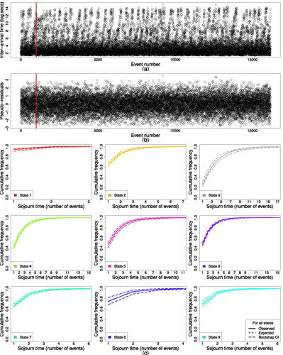
Another important assumption of HMMs is that the sojourn times in each state follow a geometric distribution. A single unit of time in our model is a LFE event. Therefore the number of events in each state should be geometrically distributed. The expected number of events along with bootstrap 99% confidence interval bounds are shown for the 9 state model in Figure 3(c) and the 13 state model in the supplementary material (Figure S2). For the 9 state HMM the observed number of events fall within these confidence bounds, and in most cases closely follow the fitted geometric line, suggesting no cause for concern regarding the model appropriateness. The plots of the number of events for the 13 state model indicate over-fitting. There was only 1 event in each visit to state 1. For many other states the vast majority of visits had only 2 events. These findings raise concerns about the usefulness of the 13 state HMM, as it requires highly frequent transitions between states.

4.2 Information Gain

We compare the selected 9 state HMM with a null model to establish the information gain from fitting the more complex model. The forecasting probability density function for x_t is defined as $$\begin{array}{c}P(X_t|X_1,\dots ,X_{t-1})=\frac{P(X_t,X_{1:(t-1)})}{P(X_{(t-1)},X_{1:(t-2)})}\\ =\frac{\sum _{i=1}^{m}P(X_t,X_{1:(t-1)},C_t=i)}{\sum _{i=1}^{m}P(X_{(t-1)},X_{1:(t-2)},C_{t-1}=i)}\\ =\frac{\sum _{i=1}^m{\alpha }_t(i)}{\sum _{i=1}^m{\alpha }_{t-1}(i)},\end{array}$$ where α_t are the forward probabilities defined as $$\begin{array}{c}{\alpha }_1(i)={\delta }_{i}f(x_1|C_t=i)\\ {\alpha }_{t+1}(i)=\sum _{j=1}^m{\alpha }_t(j){\gamma }_{ji}f(x_{t+1}|C_{t+1}=i).\end{array}$$

For the null model we assume the inter-arrival times between LFEs are independent and identically distributed random variables from a density function g(x). This is estimated by $\widehat{g}(x)=(\text{Inter-arrival times in range}(x-h,x+h))/2hT$, where T is the total number of time points (LFE events) and h varies on a fine scale between 0.01 and 0.1.

The forecasting performance is compared using the likelihood ratio of the forecasts. The probability gain for the forecast made by the 9-state HMM against the null model at time t is defined as $p_g(t)=P(X_t|X_{1:(t-1)})/g(x)$. The probability gain over the whole period can be defined by the likelihood ratio over all time points $P_g={\prod }_{t=1}^T{p}_g(t)$, and the information gain per time point (event) is $(1/T)\hspace{0.17em}\log \hspace{0.17em}{P}_g$.

For the 9 state gamma HMM the information gain per time point is 0.102, when h = 0.05. This means that compared to the null model our HMM model gained approximately $\hspace{0.17em}\exp \hspace{0.17em}(0.102)=1.11$ times more in probability per time point. The corresponding probability gain over the whole time period is 1651.017. Trying different values of h from 0.01 to 0.1 with a step of 0.002, we obtained information gain per time point of between 0.051 and 0.108.

4.3 Evolution of States

We can visualize how HMMs prioritize the classification of points by examining the sequence of state splitting. Figure 4(a) shows the state-dependent pdfs color coded by state for the 8 to 13 state gamma HMMs. The Viterbi classification of the first 500 events for each HMM is also included in the Figure 4(b). The model picks out increasingly detailed features of the behavior of LFE family 30 when the number of states increases. The equivalent plots for 5 to 7 and 14 to 16 state gamma HMMs are provided in the supplementary material (Figure S3). A graphical depiction of the state splitting sequence is also included in the supplementary material (Figure S4). This summarizes how events are re-classified as HMMs with additional states are fitted.

Fig. 4 (a) State-dependent pdfs; (b) Viterbi classified first 500 inter-arrival times, for the 8 to 13 state gamma HMMs.

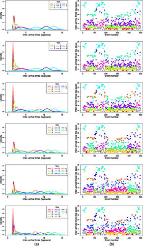
In the 5 state model (Figure S3) there is minimal overlap between the pdfs for different states. Events are classified at a crude level based largely on length of inter-arrival time, as they were when using 2–4 state HMMs (not shown). When a sixth state is included the model splits the shortest inter-arrival time points in state 1 into two. The key difference in the 7 state HMM is the almost entirely overlapping pdfs of states 2 and 3, and states 4 and 5. This model is able to separate similar inter-arrival times that are associated with different transition patterns of the Markov chain. The additional state in the 8 state model (denoted as State 7 in dark blue, Figure 4) captures activity in the range between states 6 and 7 in the 7 state model. This eighth state is important to include as it appears to mark a transition between the long inter-arrival times corresponding to lower activity states and those with consistently higher activity rates (Figure 4(b)). The ninth state separates the inter-arrival times in state 1 of the 8 state model into two states. This extra state accounts for those events which are nearly replicates. LFE detections within the same family that occurred less than 4 sec apart were considered replicates and removed from the catalog (Shelly 2017). Those events classified into state 1 have inter-arrival times only slightly above 4 sec.

The 10 state model creates an additional state by splitting state 7 of the 9 state model into two. The distributions of the four states covering the longest inter-arrival times remain largely unchanged for HMMs with 10 to 16 states, although some events are reclassified into different states. Subsequent states mostly split the events with short inter-arrival times (Figure 4(a)). The 11 state model appears to broadly classify the LFE activity into three levels, but they are not well-defined. From the 13 state model onward (Figure S3) it becomes difficult to distinguish the different pdfs for the higher activity states due to the extent to which they overlap. This suggests the HMMs are now over complicating the classification of states.

Combining the insights gained by comparing information criteria, assessments for lack-of-fit, and studying the Viterbi path and state-dependent pdfs, we can conclude that the 9 state gamma HMM is the most appropriate for LFE family 30. It appears to detect changes in the occurrence patterns of LFE activity without over-fitting. The 13 state model is more complicated. To select the more parsimonious model for classification, considering the number of events in each state follow the assumed geometric distribution (Section 4.1), the gamma model with 9 states is selected and examined in further detail.

4.4 9 State Gamma HMM: Interpreting Characteristics and Transition Patterns of States

The mean inter-arrival time in log seconds is plotted against the coefficient of variation and stationary distribution $\mathit{\delta }$ in Figure 5. The coefficient of variation is defined as $\sigma /\mu$, where σ and μ are the standard deviation and mean of the gamma state-dependent distribution. The ith element of $\mathit{\delta }$, δ_i, is the proportion of events that occur in state i as time is indexed by number of events in our model.

Fig. 5 (a) Stationary distribution against mean log inter-arrival time and (b) coefficient of variation against mean log inter-arrival time for each state of the 9 state gamma HMM fitted to family 30. Plot text indicates mean inter-arrival time on original scale.

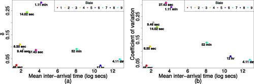
• The first state is characterized by a small number of events with short mean inter-arrival time of ∼ 4.5 sec and limited variation around this. For states with increasing mean inter-arrival times there is increasing relative variation (until state 7), and considerable oscillations in number of events.

• The second state has a mean inter-arrival time of about 6.5 sec and low variability, with the Markov chain experiencing a moderate number of events in this state (${\delta }_2\sim 0.10$).

• There are clear similarities in the distributions of LFE activity captured by states 3 and 4, and states 5 and 6, in terms of both mean inter-arrival times and coefficients of variation. However as shown in Figure 5(a), the hidden Markov chain spends much less time within states 3 and 5 compared to states 4 and 6.

• The seventh state has a mean inter-arrival time of 53 min and a reduced coefficient of variation of 0.14. A moderate amount of events take place in this state. State 8 has a mean of 12 hr between events and relatively less variation than state 7. The Markov chain has very few events here and in state 1. They appear to act as intermediaries that facilitate transitions between the other states.

• State 9 consists of the longest mean inter-arrival times, just over 4 days. This state has the second lowest coefficient of variation, slightly above that of state 1. Again it experiences few events.

• Overall, the Markov chain has less events in states with long mean inter-arrival times. That is, when the region near LFE family 30 is quiescent, there was rarely an LFE occurrence.

HMMs are powerful tools that can detect patterns not just in the distributions of event behavior, but also the time spent displaying a particular behavior. Based on the transition probabilities, the 9 state gamma HMM reveals two larger subsystems of activity. One has few events separated by long inter-arrival times, and the Markov chain displays dispersed activity over an extended stay here. The other has many events with only short inter-arrival times, where the Markov chain experiences bursts of activity for brief periods.

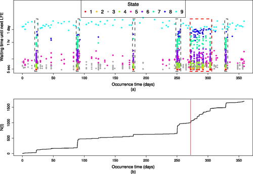
Figure 6(a) displays the inter-arrival time by occurrence time for events observed during 2004. Figure 6(b) shows the cumulative number of events over the same period. This allows us to examine how variations in recurrence behavior are distributed over time. This is especially important when analyzing point process data which consists of events occurring at random times. The Viterbi classified sequence and cumulative plot of all observed events can be found in the supplementary material (Figure S5), however the cyclic behavior detected by the model is not clear in this initial plot and it appears events have been classified based on inter-arrival times alone. Examining a portion of the classified data, such as the first year, reveals more detail.

Fig. 6 LFE events in family 30 recorded during the year 2004. (a) Inter-arrival times against occurrence time with events classified by the Viterbi algorithm, gray boxes enclose events in subsystem 2 and red box encloses cluster of activity following Parkfield earthquake. (b) Cumulative number of events against occurrence time. Red line indicates occurrence of 2004 Parkfield earthquake.

We are able to confirm the existence of two distinct subsystems of activity, as indicated in the plots of the classified points based on the Viterbi path and the characteristics of state-dependent distributions, using transition probability plots (Figure 7). Darker purple indicates relatively higher transition probabilities between states 3, 5, 8, 9 and likewise between states 1, 2, 4, 6, 7, comprising the first and second subsystems (most clearly shown in Figure 7(b)). The uncertainty in the transition probability estimates is small based on confidence intervals calculated via bootstrap simulation. The margins of error are symmetric and less than 0.02, and maintain the subsystem relationships between states. The subsystems are also shown in Figure 6(a).

Fig. 7 Transition probabilities between states, with states on y axis transitioning to states on x axis. Best estimate of transition probabilities in (b) bounded by margins of error—distance to lower (a) and upper (c) 95% bootstrap confidence interval bounds.

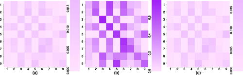
The majority of the points in subsystem 1 occur in the high activity state 3. State 5 appears to represent an intermediate state of the LFE process, the transition between active (short inter-arrival times) periods of state 3 and quiescent (long inter-arrival times) of state 9. State 8 occurs relatively rarely but appears to be a connecting state between the two subsystems. It has a close relationship with states 3, 5, and 9 in the first subsystem, and is also likely to transition to state 6 in subsystem 2.

Within subsystem 2 there is less variation as all states display reasonably high activity rates. State 1 incorporates near over-lapping events throughout the observation period. State 2 has a close relationship with state 4, and together they represent similar activity to that in state 3 in the first subsystem. However, state 4 generates more events than state 2 with almost triple the average number of events per visit. A considerable amount of the transitions out of state 4 come to state 6. This state has a high self-transition probability and transitions to other states in the subsystem with roughly equal probabilities. State 7 generates the longest inter-arrival times in the second subsystem. It tends to transition to either state 6 or itself.

The long periods with limited activity (where the cumulative number of events does not increase notably) correspond to the chain being in the first subsystem. The sharp increases in activity, where the cumulative number of events climbs rapidly in a short amount of time, correspond to the chain being in the second subsystem.

Subsystem 1 is the more variable of the two. It contains regular bursts that may be considered background activity, separated by the longest inter-arrival times. The role of state 8 as a transition between the subsystems is apparent as it captures events on the border (Figure 6(a)). Substantial activity takes place when the chain is in subsystem 2, demonstrated by the tightly clustered events in Figure 6(a) and jumps in cumulative number of events (Figure 6(b)). The chain does not spend as long here but makes up for it with rapidly occurring events. The longest inter-arrival times in subsystem 2 are about 6 hr.

As shown in Figure 6(a), the hidden Markov chain transitions between subsystems as the Parkfield earthquake takes place. Before this earthquake family 30 was experiencing a cluster of events in states 3 and 5 of subsystem 1. Immediately following the Parkfield event family 30 transitioned to a burst of activity within subsystem 2, generating many events from state 4. This was followed by an accelerated sequence of transitions between subsystems 1 and 2 lasting about a month. The system then returned to recurrence patterns displayed earlier in the observation period. This pattern of activity was maintained by family 30 throughout years 2004 to 2016, plots equivalent to Figure 6 for the years 2005–2007 are in the supplementary material (Figures S6–S8).

4.5 Subsystems as a Markov Chain

It is possible to conceptualize the movement between the two subsystems as a Markov chain with a discrete binary state space $i=\{1,2\}$ representing subsystems 1 and 2, and discrete index set corresponding to LFE event number $t=\{1,\dots ,n\}$.

The estimated transition probability from subsystem 1 to subsystem 2 is 0.0212, and that from subsystem 2 to 1 is 0.0083. Between-subsystem transitions are more than twice as likely from subsystem 1 to subsystem 2 as vice versa. This is reflected in more than 70% of LFE events occurring in subsystem 2, leaving less than 30% in subsystem 1.

The observed number of events by subsystem is plotted in the supplementary material (Figure S9). The expected number of events if a geometric distribution was followed along with bootstrap 99% confidence interval bounds is shown. The observed number of events for each state fall within these confidence bounds and in most cases closely follow the fitted geometric line. Based on these measures it appears the assumption of geometrically distributed number of events is satisfied.

5 Conclusions and Discussion

This article has explored the usefulness of HMMs coupled with visualization techniques to analyze the recurrence patterns displayed by an episodic LFE family along the San Andreas Fault. We find family 30 alternates between episodic bursts and quiescent behavior with repeating activity patterns over time. The predominantly cyclic nature of LFE recurrence, and the Parkfield earthquake’s effect on this, is both detected and shown in finer detail by the 9 state gamma HMM. Plots highlight the behaviors corresponding to low and high LFE activity, and identify a transitional state that signals a change in activity level. The geological sources of this behavior are hypothesized to be related to changes in fault friction or pore pressure (Veedu and Barbot 2016; Shelly 2017). This is a step toward linking these patterns of behavior to underlying slow slip events. The success of this application motivates HMMs as a tool for investigating further LFE activity, both in additional San Andreas locations and along other faults.

The 8 state gamma HMM is distinguished from the 9 state model based on the partitioning of events with the shortest and least variable inter-arrival times. Visualizing the state dependent distributions shows the two states with the shortest inter-arrival times in the 9 state HMM have similar means, differing by only 1.5 sec, although the newly created second state has increased variability. This leaves very few observed events in state 1 of the 9 state HMM. The adjusted BIC measure indicates a definitive preference for the 9 state model. One possible explanation for isolating these events is that an inter-arrival time of only 4.5 sec, or less, comes close to the cutoff of 4 sec used by Shelly (2017) to determine duplicate events. It may be that the additional state is isolating events where there is almost negligible separation and potentially overlap.

As shown by graphical techniques implemented in Section 4, in the 9 state gamma HMM there are two distinct subsystems of activity. Subsystem 1 experiences small episodes of activity separated by quiescent periods. By plotting this adjacent to the observed data we see this corresponds to an almost stable cumulative number of LFE events with occasional jumps. There are around 46 events on average here before the chain moves to subsystem 2, usually taking a couple of months. Shelly (2017) observes that changes from episodic to continuous behavior often correspond to increases in LFE activity rate. This is clearly demonstrated in plots of family 30, with subsystem 2 characterized by consistent surges of activity containing roughly 2.5 times as many events as subsystem 1.

It is not entirely clear which geological processes underlie the different subsystems. The change in activity may be a result of differences in rate-dependent friction on the fault, with the surge in LFE production seen in subsystem 2 corresponding to an external increase in loading. Alternatively, these surges may be a consequence of changes in friction or pore pressure (Shelly 2017). Family 30 displays a consistent step-like increase in cumulative number of events between 2004 and 2016. This suggests that the processes moderating LFEs within this family have some sort of cyclic behavior. Following the Parkfield earthquake the fitted 9 state HMM model maintained episodic and quiescent subsystems, the increased activity was captured by these alternating on a faster timescale. This suggests that rather than a unique post-earthquake mechanism arising, existing LFE generating processes were temporarily accelerated by the large earthquake. The behavior of other LFE families, in particular the migration of activity between families, may also have a role in moderating these processes. An advanced multi-level HMM could be developed for LFEs, in which the observed data are conditioned upon a Markov chain that is then conditioned on another Markov chain describing the subsystems. Our post-fitting visualization is able to uncover this extra layer of information without fitting a more complicated model.

The 88 San Andreas families each generate thousands of LFE events a year and display diverse patterns of activity. In addition to fitting further HMMs to these locations, additional analysis methods should be explored to uncover spatial patterns of LFE behavior in this region. In this article, the dependence between events in family 30 is captured by a first-order HMM. For future research on LFEs or applying this model to other point process data with recurrence patterns of clustered events, if the dependence between events cannot be adequately captured by a first-order HMM, one can consider modeling dependence directly within the HMM framework. That is, conditioning on the hidden Markov chain, the observed inter-arrival times can be modeled by an autoregressive type of models.

Acknowledgments

The authors wish to thank Jodie Buckby for sharing code to fit and optimize hidden Markov models, and providing general assistance. We are grateful to Marco Brenna for advice regarding geological interpretations, visualization, and additional edits. The authors also wish to acknowledge the use of New Zealand eScience Infrastructure (NeSI) high performance computing facilities and consulting support as part of this research. New Zealand’s national facilities are provided by NeSI and funded jointly by NeSI’s collaborator institutions and through the Ministry of Business, Innovation & Employment’s Research Infrastructure program. URL https://www.nesi.org.nz. The authors acknowledge the suggestions of two anonymous reviewers in enhancing this article.

Supplementary Materials

The supplementary material contains (i) R code used for the analysis, (ii) tables of results for gamma, Weibull, log-normal and normal hidden Markov models in Section 4.1, (iii) additional pseudo-residual plots and sojourn checks for Section 4.1, (iv) additional probability density plots and plot of state splitting sequence for Section 4.3, (v) Viterbi path visualizations for the entire observation period and years 2005, 2006, and 2007 for Section 4.4, (vi) sojourn checks for subsystems in Section 4.5.

Disclosure Statement

The authors report that there are no competing interests to declare.

References

- Bacci, S., Pandolfi, S., and Pennoni, F. (2014), “A Comparison of Some Criteria for States Selection in the Latent Markov Model for Longitudinal Data,” Advances in Data Analysis and Classification, 8, 125–145. DOI: 10.1007/s11634-013-0154-2.
- Bebbington, M., and Harte, D. (2003), “The Linked Stress Release Model for Spatio-Temporal Seismicity: Formulations, Procedures and Applications,” Geophysical Journal International, 154, 925–946. DOI: 10.1046/j.1365-246X.2003.02015.x.
- Bebbington, M. S. (2007), “Identifying Volcanic Regimes Using Hidden Markov Models,” Geophysical Journal International, 171, 921–942. DOI: 10.1111/j.1365-246X.2007.03559.x.
- Bhaduri, M. (2020), “On Modifications to the Poisson-Triggered Hidden Markov Paradigm through Partitioned Empirical Recurrence Rates Ratios and its Applications to Natural Hazards Monitoring,” Scientific Reports, 10, 1–19. DOI: 10.1038/s41598-020-72803-z.
- Borchers, D. L., and Langrock, R. (2015), “Double-Observer Line Transect Surveys with Markov-Modulated Poisson Process Models for Animal Availability,” Biometrics, 71, 1060–1069. DOI: 10.1111/biom.12341.
- Bray, A., and Schoenberg, F. P. (2013), “Assessment of Point Process Models for Earthquake Forecasting,” Statistical Science, 28, 510–520. DOI: 10.1214/13-STS440.
- Buckby, J., Wang, T., Zhuang, J., and Obara, K. (2020), “Model Checking for Hidden Markov Models,” Journal of Computational and Graphical Statistics, (4), 859–874. DOI: 10.1080/10618600.2020.1743295.
- Buckby, J. J. (2020), “Model Selection and Model Checking for Hidden Markov Models Applied to Non-Volcanic Tremor Data,” Master’s Thesis, University of Otago. Available at http://hdl.handle.net/10523/10382.
- Costa, M., and De Angelis, L. D. (2010), “Model Selection in Hidden Markov Models: A Simulation Study,” in No 7, Quaderni di Dipartimento. Department of Statistics, University of Bologna.
- Escola, S., Fontanini, A., Katz, D., and Paninski, L. (2011), “Hidden Markov Models for the Stimulus-Response Relationships of Multistate Neural Systems,” Neural Computation, 23, 1071–1132. DOI: 10.1162/NECO_a_00118.
- Hannan, E. J., and Quinn, B. G. (1979), “The Determination of the Order of An Autoregression,” Journal of the Royal Statistical Society, 41, 190–195. DOI: 10.1111/j.2517-6161.1979.tb01072.x.
- Ho, C.-H., and Bhaduri, M. (2015), “On a Novel Approach to Forecast Sparse Rare Events: Applications to Parkfield Earthquake Prediction,” Natural Hazards, 78, 1–27. DOI: 10.1007/s11069-015-1739-1.
- Holzmann, H., and Schwaiger, F. (2016), “Testing for the Number of States in Hidden Markov Models,” Computational Statistics and Data Analysis, 100, 318–330. DOI: 10.1016/j.csda.2014.06.012.
- Ignatieva, A., Bell, A. F., and Worton, B. J. (2018), “Point Process Models for Quasi-Periodic Volcanic Earthquakes,” Statistics in Volcanology, 4, 1–27. arXiv:1803.07688v2. DOI: 10.5038/2163-338X.4.2.
- Kahle, D., and Wickham, H. (2013), “ggmap: Spatial Visualization with ggplot2,” The R Journal, 5, 144–161. Available at https://journal.r-project.org/archive/2013-1/kahle-wickham.pdf. DOI: 10.32614/RJ-2013-014.
- Lu, S. (2012), “Markov Modulated Poisson Process Associated with State-Dependent Marks and its Applications to the Deep Earthquakes,” Annals of the Institute of Statistical Mathematics, 64, 87–106. DOI: 10.1007/s10463-010-0302-9.
- Massey, F. J. (1951), “The Kolmogorov-Smirnov Test for Goodness of Fit,” Journal of the American Statistical Association, 46, 68–78. DOI: 10.2307/2280095.
- McClintock, B. T., Langrock, R., Gimenez, O., Cam, E., Borchers, D. L., Glennie, R., and Patterson, T. A. (2020), “Uncovering Ecological State Dynamics with Hidden Markov Models,” Ecology Letter, 23, 1878–1903. DOI: 10.1111/ele.13610.
- Michel, S., Jolivet, R., Lengliné, O., Gualandi, A., Larochelle, S., and Gardonio, B. (2022), “Searching for Transient Slow Slips Along the San Andreas Fault Near Parkfield Using Independent Component Analysis,” Journal of Geophysical Research: Solid Earth, 127, e2021JB023201. DOI: 10.1029/2021JB023201.
- Obara, K. (2011), “Characteristics and Interactions between Non-volcanic Tremor and Related Slow Earthquakes in the Nankai Subduction Zone, Douthwest Japan,” Journal of Geodynamics, 52, 229–248. DOI: 10.1016/j.jog.2011.04.002.
- Obara, K., and Kato, A. (2016), “Connecting Slow Earthquakes to Huge Earthquakes,” Science, 353, 253–257. DOI: 10.1126/science.aaf1512.
- Ogata, Y. (1988), “Statistical Models for Earthquake Occurrences and Residual Analysis for Point Processes,” Journal of the American Statistical Association, 83, 9–27. DOI: 10.1080/01621459.1988.10478560.
- Peterson, C., and Christensen, D. (2009), “Possible Relationship between Non-volcanic Tremor and the 1998-2001 Slow-Slip Events, South Central Alaska,” Journal of Geophsyical Research, 114, B06302. DOI: 10.1029/2008JB006096.
- Pohle, J., Langrock, R., van Beest, F., and Schmidt, N. M. (2017), “Selecting the Number of States in Hidden Markov Models: Pragmatic Solutions, Illustrated Using Animal Movement,” Journal of Agricultural, Biological and Environmental Statistics, 22, 270–293. DOI: 10.1007/s13253-017-0283-8.
- R Core Team. (2020), R: A Language and Environment for Statistical Computing, Vienna, Austria: R Foundation for Statistical Computing. Available at https://www.R-project.org/.
- Rogers, G., and Dragert, H. (2003), “Episodic Tremor and Slip on the Cascadia Subduction Zone: The Chatter of Silent Slip,” Science, 300, 1942–1943. DOI: 10.1126/science.1084783.
- Rousset, B., Bürgmann, R., and Campillo, M. (2019), “Slow Slip Events in the Roots of the San Andreas Fault,” Science Advances, 5, eaav3274. DOI: 10.1126/sciadv.aav3274.
- Shcherbakov, R., Zhuang, J., Zöller, G., and Ogata, Y. (2019), “Forecasting the Magnitude of the Largest Expected Earthquake,” Nature Communications, 10, 4051. DOI: 10.1038/s41467-019-11958-4.
- Shelly, D. R. (2017), “A 15 Year Catalog of More than 1 Million Low-Frequency Earthquakes: Tracking Tremor and Slip Along the Deep San Andreas Fault,” Journal of Geophysical Research: Solid Earth, 122, 3739–3753. DOI: 10.1002/2017JB014047.
- Shelly, D. R., and Hardebeck, J. L. (2010), “Precise Tremor Source Locations and Amplitude Variations Along the Lower-Crustal Central San Andreas Fault,” Geophysical Research Letters, 37, L14301. DOI: 10.1029/2010GL043672.
- Shelly, D. R., and Johnson, M. K. (2011), “Tremor Reveals Stress Shadowing, Deep Postseismic Creep, and Depth-Dependent Slip Recurrence on the Lower-Crustal San Andreas Fault Near Parkfield,” Geophysical Research Letters, 38, L13312. DOI: 10.1029/2011GL047863.
- Supino, M., Poiata, N., Festa, G., Vilotte, J. P., Satriano, C., and Obara, K. (2020), “Self-Similarity of Low-Frequency Earthquakes,” Scientific Reports, 10, 6523. DOI: 10.1038/s41598-020-63584-6.
- Thomas, A. M., Beeler, N. M., Bletery, Q., Burgmann, R., and Shelly, D. R. (2018), “Using Low-Frequency Earthquake Families on the San Andreas Fault as Deep Creepmeters,” Journal of Geophysical Research: Solid Earth, 123, 457–475. DOI: 10.1002/2017JB014404.
- Tokdar, S., Xi, P., Kelly, R. C., and Kass, R. E. (2009), “Detection of Bursts in Extracellular Spike Trains Using Hidden Semi-Markov Point Process Models,” Journal of computational neuroscience 29, 203–212. DOI: 10.1007/s10827-009-0182-2.
- Ushey, K., Allaire, J., Wickham, H., and Ritchie, G. (2020), rstudioapi: Safely Access the RStudio API, available at https://github.com/rstudio/rstudioapi.
- van der Elst, N. J., Delorey, A. A., Shelly, D. R., and Johnson, P. A. (2016), “Fortnightly Modulation of San Andreas Tremor and Low-Frequency Earthquakes,” Proceedings of the National Academy of Sciences of the United States of America, 113, 8601–8605. DOI: 10.1073/pnas.1524316113.
- Veedu, D. M., and Barbot, S. (2016), “The Parkfield Tremors Reveal Slow and Fast Ruptures on the Same Asperity,” Nature, 532, 361–365. DOI: 10.1038/nature17190.
- Viterbi, A. J. (1967), “Error Bounds for Convolutional Codes and An Asymptotically Optimum Decoding Algorithm,” IEEE Transactions on Information Theory, 13, 260–269. DOI: 10.1109/TIT.1967.1054010.
- Wang, T., and Bebbington, M. (2012), “Estimating the Likelihood of an Eruption from a Volcano with Missing Onsets in its Record,” Journal of Volcanology and Geothermal Research, 243–244, 14–23. DOI: 10.1016/j.jvolgeores.2012.06.032.
- Wang, T., Bebbington, M., and Harte, D. (2012), “Markov-Modulated Hawkes Process with Stepwise Decay,” Annals of the Institute of Statistical Mathematics, 64, 521–544. DOI: 10.1007/s10463-010-0320-7.
- Wang, T., Zhuang, J., Buckby, J., Obara, K., and Tsuruoka, H. (2018), “Identifying the Recurrence Patterns of Non-volcanic Tremors Using a 2d Hidden Markov Model with Extra Zeros,” Journal of Geophysical Research: Solid Earth, 123, 6802–6825. DOI: 10.1029/2017JB015360.
- Wang, T., Zhuang, J., Obara, K., and Tsuruoka, H. (2017), “Hidden Markov Modelling of Sparse Time Series from Non-volcanic Tremor Observations,” Journal of the Royal Statistical Society, Series C, 66, 691–715. DOI: 10.1111/rssc.12194.
- Wang, Y., Wang, T., and Zhuang, J. (2018), “Modeling Continuous Time Series with Many Zeros and An Application to Earthquakes,” Environmetrics, 29, e2500. DOI: 10.1002/env.2500.
- Wu, C., Guyer, R., Shelly, D., Trugman, D., Frank, W., Gomberg, J., and Johnson, P. (2015), “Spatial-Temporal Variation of Low-Frequency Earthquake Bursts Near Parkfield, California,” Geophysical Journal International, 202, 914–919. DOI: 10.1093/gji/ggv194.
- Wu, C., Shelly, D. R., Gomberg, J., Peng, Z., and Johnson, P. (2013), “Long-term Changes of Earthquake Inter-Event Times and Low-Frequency Earthquake Recurrence in Central California,” Earth and Planetary Science Letters, 368, 144–150. DOI: 10.1016/j.epsl.2013.03.007.
- Zucchini, W., and MacDonald, I. (2009), Hidden Markov Models for Time Series: An Introduction Using R, New York: Chapman and Hall/CRC.