A metaheuristic approach for interval type-2 fuzzy fractional order fault-tolerant controller for a class of uncertain nonlinear system*

Abstract

A new optimum interval type-2 fuzzy fractional-order controller for a class of nonlinear systems with incipient actuator and system component faults is introduced in this study. The faults of the actuator and system component (leak) are taken into account using an additive model. The Interval Type-2 Fuzzy Sets (IT2FS) is used to design an optimal fuzzy fractional order controller, and two different nature inspired metaheuristic algorithms, Follower Pollination Algorithm (FPA) and Genetic Algorithm (GA), are used to optimize the parameters of the fuzzy PID controller and Interval Type-2 Fuzzy Tilt-Integral-Derivative Controller (IT2FTID) for nonlinear system. The suggested control approach consists of two parts: an Interval Type-2 Fuzzy Logic Controller (IT2FLC) controller and a fractional order TID controller. Additionally, the two inputs of the IT2FLC are also calibrated using two fine tuning parameters ${\text{β}}_1$ and ${\text{β}}_2$, respectively. The stability of the proposed controller is presented with some conditions. In addition to unknown dynamics, some unknown process disturbances, such as rapid changes in the control variable, are taken into account to check the efficacy of the proposed control scheme. Two nonlinear conical two-tank level systems are used in the simulation as a case study. The performance of the suggested approach is also compared to that of a widely recognized Interval Type-2 Fuzzy Proportional-Integral-Derivative (IT2FPID) Controller. Finally, the proposed control scheme's fault-tolerant behaviour is demonstrated using fault-recovery time results and statistical Z-tests for both controllers, and the proposed IT2FTID controller's effectiveness is demonstrated when compared to IT2FPID and existing passive fault tolerant controllers in recent literature.

Keywords:

• Actuator fault
• conical two-tank
• follower pollination algorithm
• genetic algorithm
• interval type-2 fuzzy system
• system component fault
• tilt-integral-derivative controller
• frustum two-tank
• fuzzy fault-tolerant control

1. Introduction

Due to the intricacy of problems, solving them using traditional procedures in a fair amount of time becomes difficult. Metaheuristic strategies have been developed in recent years to address this issue. The strategies can handle complex issues in an acceptable amount of time. Metaheuristic strategies are based on concepts from biological science, physics, animal and insect behaviour, and other fields [1]. In the literature, a variety of metaheuristic algorithms have been created. Genetic algorithm (GA), ant colony optimization (ACO), follower pollination algorithm (FPA), particle swarm optimization (PSO), grey wolf optimization (GWO), harmony search algorithm (HSA), and many others are examples of well-known methodologies. Follower Pollination Algorithm (FPA) is recently developed and a well-known metaheuristic algorithm, which is proposed by Yang in 2012 [2] in 2012. Additionally, interval type-2 fuzzy logic has been shown to be one of the most cited and used methods in the field of robotics and control due to better ability to handle uncertainty and adding human intelligence based on expertise. And hence, we proposed FPA-based interval type-2 fuzzy fractional order fault-tolerant controller for uncertain nonlinear system.

The control of the nonlinear systems (NSs) in presence of unmodelled dynamics (NSs-UD) and in faulty situation are one of the most challenging problems in control engineering. The problem of the uncertain parameters or uncertain functions in the dynamics of the nonlinear systems have been considered in adaptive control techniques, but the problem of the control of NSs with faulty situation has been quite rarely investigated in literature, and thereafter we proposed optimal fuzzy fault-tolerant controller using IT2FTID with FPA metaheuristic approach.

One of the real-world second-order systems (SOS) [3–7] frequently utilized in many industrial production processes [8] is the two-tank level control system. According to the literature, the PID controller [8,9], fuzzy controller [8], fuzzy-PID controller [10], and neural network [11,12] can effectively control the level of a non-interacting (single-tank, two-tank) system. For single-tank or multi-tank level control, the PID controller is the most popular and straight forward method. The PID design problem for the non-interacting level control system can be considered one of the constrained optimization problems that can be efficiently solved by metaheuristic algorithms in today's optimization context. For illustration, the design of a PID controller for the non-interacting level control system using the Genetic Algorithm (GA) algorithm [13], or Particle Swarm Optimization (PSO) [14,15]. However, that author has recently used interval type-2 fuzzy logic controllers, Takagi Sugeno fuzzy logic controllers, and several of the control techniques provided in [16–19] for interacting level control processes under various conceivable system faults.

Due to the limited flexibility of tuning settings, traditional PID control performance degrades dramatically when actuator, system component (leak), and sensor defects, modelling uncertainty, and process disruptions occur in the system [20]. As a result, a Titled Derivative Integrator (TID) controller [21,22] was developed, which has four tuning parameters $K_P$, $K_I$, $K_D$, and n, allowing for additional flexibility in controlling the nonlinear system. Interval type-2 FLC is utilized in this article to add more tuning parameters so that it can manage and produce quick and smooth responses for higher-order plants than a traditional PID controller. Modelling uncertainty, defects, and process disruptions are all handled by the IT2FTID.

Furthermore, a nonlinear model that accurately represents plant activity is first established. A classic integer order PID control strategy is developed based on this model representation of the plant, with parameters tuned using the Genetic Algorithm (GA) and Ziegler & Nichols (ZN) methods and a linearized model at three different operating points, similar to what was done in some preliminary works, both from simulation and experimental viewpoints [23]. The controller parameters are optimized using Ziegler & Nichols (ZN) and Genetic Algorithm (GA) [23]. Then, integer order PID control strategies and their fractional order equivalents, fractional order PID (FOPID), are created. In addition, any common method for tuning the fractional order PID and integer order PID for nonlinear systems is covered in [24]. Interval type-2 fuzzy state machines have recently been used to create active fault-tolerant control for stochastic system models [24].

Several studies in the literature have framed the PID tuning problem as an optimization problem with the goal of improving the closed-loop system's performance through decentralized PID tuning. The concept of Gershgorin bands was used in [25] to define a nonlinear optimization problem with stability margin requirements, although the solution was limited to weakly coupled processes. A nonlinear optimization issue was formulated in [26], but the constraints were connected to performance indicators such as maximum overshoot and maximum controller limit deviation for each loop; overall stability for the MIMO closed-loop system was not considered. Two linear programming approaches to computing PID parameters were proposed in [27], where the loop interactions were taken into account by the Gershgorin bands and the effective open-loop process notion, but each loop had to be tuned separately.

In contrast to the previously stated decentralized techniques, centralized PID systems are generally implemented using a decoupler or another mathematical instrument that attempts to eliminate variable coupling effects. Due to the necessity to know the process model in order to construct the decoupler, a decoupler makes the control system structure more complex and highly dependent on the plant models. In [28], author investigated TITO (Two-Input Two-Output) systems with centralizsed PID control. The authors present an approach that uses model approximations to develop PI controllers for the main diagonal and decouplers for off-diagonal dynamics.

Lakshmanaprabu et al. [29] designed a fractal PI/PID controller for TITO using an evolutionary algorithm (bat algorithm) in the style of multiobjective optimization. The design and tuning of a PI controller for a nonlinear TITO process was examined in [30] using multiple optimization methodologies such as a genetic algorithm (GA) and particle swarm optimization (PSO). According to the authors, the GA produces better tracking performance and less overshoot in the nonlinear scenario than the PSO-based approach. This result may indicate that a GA is preferable for tuning purposes in the presence of high nonlinearities and model mismatch. PID controller tuning methods based on nonlinear optimization and linear prgmarmming have recently been proposed in [31,32], as well as the design and implementation challenges of PI/PID controllers resulting from decomposing MIMO systems into single loops. However, in the recent decade, a new metaheuristic algorithm based on the flower pollination process of flowering plants has emerged and proven popular. Pollen transfer is commonly related with flower pollination, and such transfer is frequently associated with pollinators such as insects, birds, bats, and other animals. Previous studies imply that the FPA improves the performance of existing biologically inspired algorithms such as GA, ABC, PSO, and others, including the CS, which is currently getting a lot of attention from the research community due to its effectiveness and minimal parameter settings [32–35]. For variable speed drive systems and induction motor seed control, authors presented optimal tuning of PI controllers utilising flower pollination optimization algorithms in [33,34]. In addition, for PI controller parameters optimization for chemical processes, such as heat exchanger processes, researchers employed metaheuristic optimization algorithms such as bat algorithms, particle swarm optimization algorithm, and flower pollination algorithm in [35].

This study focuses on developing a technique for designing an IT2FTID for fault-tolerant controller using FPA. Differentiating capabilities of IT2FTID and IT2FPID in terms of modelling uncertainty, fault tolerance, and disturbance rejection are also achieved. The following is the order of the rest of the article: Preliminaries and a singleton type-2 FLC are described in Section III. In part II, the mathematical model for a two-tank non-interacting conical tank system is presented. In Section IV, the mathematical model of FPOA and its characteristic are shown. The IT2FTID/IT2FPID control strategy for a conical two-tank non-interacting level control process presented in Section V is compared to simulation findings in Section VII to see how well it can handle modelling uncertainties, faults, and process disruptions. In section VI, presents the stability analysis of the fractional order TID controller with mathematical equations. Finally, in Section VIII, conclusions are formed.

1.1. Motivations and contributions

Fuzzy sets have been used to optimize the strategic parameters of various metaheuristic algorithms in recent years because fuzzy inference systems aid in understanding and working with human knowledge bases, resulting in significant improvements in the efficacy of the various metaheuristic algorithms [18,22,23]. Also the metaheuristic algorithms are used to optimization of the standard mathematical functions, controller's parameters, or various kind of engineering or non-engineering optimization problems, and therefore described work is based on nature inspired metaheuristic Flower Pollination Algorithm (FPA) for engineering control system.

Because of its potential to solve the optimal problem in engineering and non-engineering applications, the flower pollination algorithm has gotten a lot of attention since its conception. The FPA is now the best method for improving the controller parameters of interval type-2 fuzzy integer order PID and fractional order TID controllers.

The following is the paper's major contribution:

• A metaheuristic algorithm (FPA) is used to optimize the controller parameters

• Interval type-2 fuzzy sets are utilized to design PID and TID controllers that effectively accommodate modelling and parameter uncertainty

• Additionally, two fine tuning parameters are used ${\text{β}}_1$ and ${\text{β}}_2$, which tuned the two inputs of the interval type-2 fuzzy inference system one is error e and the second is derivative of the error $\dot{e}$

• Because the fractional order TID controller has four tuning parameters, it improves the nonlinear system's control responses (i.e. transient and steady state).

• Nature inspired metaheuristic algorithm is used to find optimum controller (Fuzzy IT2TID and IT2PID) parameters

• Two different nonlinear uncertain level control processes are used to validate the proposed control scheme, and the findings are presented with actuator and system component (leak) faults

• Fault-tolerant capability of the proposed IT2-FTID controller is compared with IT2-FPID controls for nonlinear level control processes using Fault Recovery $T_{fr}$ time

• We tuned the controller using well-known metaheuristic methods, Genetic Algorithms (GA), Flower Pollination Optimization (FPO), for nonlinear level control system with higher uncertainty in terms of magnitude and abrupt nature.

• Furthermore, we confirm that the FPO technique has not been applied for fault-tolerant controller optimization for uncertain nonlinear systems in recent times.

2. Nonlinear uncertain level control system with description

2.1. Two-tank conical non-Interacting level system with mathematical model

The schematic diagram of the structural model of the Tow-tank Conical Non-Interacting Level System (TTCNILS) is demonstrated in Figure 1, which is a benchmark problem for a number of research topics. It subsists of an inverted two conical tank with an inlet flow $\left(f_1\right)$ at the top, an outlet flow from conical tank 1 $\left(f_2\right)$ at the bottom, and tank 2 outlet flow $\left(f_3\right)$ from the bottom, a pump that distributes the liquid flow, and a control valve (CV ) with coefficient $\left(\text{β}\right)$ to manipulate $\left(f_1\right)$. The valve $\left(V_1\right)$ is a manual valve which is controlled at a constant flow rate $\left(f_2\right)$ to the tank 2 and valve $\left(V_2\right)$ is a manual valve which is controlled at a constant flow rate $\left(f_3\right)$. The operating parameters of the Conical Tank system are displayed in Table 1.

Figure 1. Prototype model of TTCNILS [3] .

Table 1. Operating parameters of the TTCNILS process.

Parameter	Description	Value
R	Top radius of the conical tank	40 cm
H	Maximum height of the tank	80 cm
$f_1$	Maximum in flow to the tank 1	2.7675e–4 m${}^3$/sec
${\text{β}}_1$	Valve coefficient $\left(V_1\right)$	0.03613 cm${}^3$/sec
${\text{β}}_2$	Valve coefficient $\left(V_1\right)$	0.01923 cm${}^3$/sec
$h_1$	Steady state height of tank 1	42 cm
$h_2$	Steady state height of tank 2	31 cm
g	gravitational acceleration	981 cm/s${}^2$

The TTCNILS Process is a single input single output (SISO) non-interacting processes, in which the tank 2 liquid level $\left(h_2\right)$ is treated as the measured variable, and the inlet flow $\left(f_1\right)$ is treated as the manipulated variable. The radius (r) of the tank is a changing parameter; so it is revealed as the ratio of the maximum radius (R) to the maximum height (H) of the Conical Tank. All the TTCNILS parameters are considered in table 1 is from real-time object.

2.2. Modelling of tow-tank conical non-interacting level system

For determining the mathematical model of Two-tank conical, non-interacting level system (TTCNILS) process, first we consider a single conical tank system (CTS) which is depicted in Figure 2.

Figure 2. Prototype model of conical shape coupled-tank system [58].

The mathematical model of the CTS is given by conferring to mass balance equation (1) $\begin{array}{rl}& \mathrm{R}\mathrm{a}\mathrm{t}\mathrm{e}\mathrm{o}\mathrm{f}\mathrm{A}\mathrm{c}\mathrm{c}\mathrm{u}\mathrm{m}\mathrm{u}\mathrm{l}\mathrm{a}\mathrm{t}\mathrm{i}\mathrm{o}\mathrm{n}=\mathrm{i}\mathrm{n}\mathrm{f}\mathrm{l}\mathrm{o}\mathrm{w}-\mathrm{o}\mathrm{u}\mathrm{t}\mathrm{f}\mathrm{l}\mathrm{o}\mathrm{w}\\ & \frac{\mathrm{d}\left(M\right(h\left)\right)}{\mathrm{d}\mathrm{t}}={\rho }_1\left(f_1\right)-{\rho }_2\left(f_o\right)\end{array}$(1) Where $M\left(h\right)=\rho V\left(h\right)$ $V\left(h\right)$ is the volume of liquid in the tank, ρ is the density of liquid in the tank, ${\rho }_1$ is the density of liquid in the inlet stream and ${\rho }_2$ is the density of liquid in the outlet stream. Assuming room temperature as constant, density of liquid is same throughout. (2) $\begin{array}{rl}& {\rho }_1={\rho }_2=\rho \\ & \frac{\mathrm{d}\mathrm{V}\left(h\right)}{\mathrm{d}\mathrm{t}}=f_1-f_o\end{array}$(2) The volume of the liquid inside the conical tank at any height (h) given by: (3) $V\left(h\right)=\frac{\pi r^{2}h}{3}$(3) From Figure 2, a relation between conical tank height (H) and a top radius of conical tank (R) is given by Equation (15(15) $Vol=\frac{\pi }{3}(r_b^2+r^2+r_{b}r)$(15) ). (4) $\tan \theta =\frac{R}{H}$(4) At any level (h) (5) $\tan \theta =\frac{r}{h}$(5) Equating (15(15) $Vol=\frac{\pi }{3}(r_b^2+r^2+r_{b}r)$(15) ) and (16(16) $r=r_b+\frac{(R-r_b)}{H}h$(16) ) (6) $r=\frac{Rh}{H}$(6) Substitute (17(17) $\frac{\mathrm{d}{\mathrm{h}}_1}{\mathrm{d}\mathrm{t}}=\frac{f_{in1}-f_{o1}-f_{12}}{\frac{\pi }{3}[3r_{b1}^2+6r_{b1}\left(\frac{R-r_{b1}}{H_1}\right)h_1+3{\left(\frac{R-r_{b1}}{H_1}\right)}^2{h_1}^2]}$(17) ) in (14(14) $\begin{array}{rl}& \mathrm{R}\mathrm{a}\mathrm{t}\mathrm{e}\mathrm{o}\mathrm{f}\mathrm{A}\mathrm{c}\mathrm{c}\mathrm{u}\mathrm{m}\mathrm{u}\mathrm{l}\mathrm{a}\mathrm{t}\mathrm{i}\mathrm{o}\mathrm{n}=\mathrm{i}\mathrm{n}\mathrm{f}\mathrm{l}\mathrm{o}\mathrm{w}-\mathrm{o}\mathrm{u}\mathrm{t}\mathrm{f}\mathrm{l}\mathrm{o}\mathrm{w}\\ & \frac{\mathrm{d}\left(Vol\right)}{\mathrm{d}\mathrm{t}}=f_{in}-f_o\end{array}$(14) ) (7) $V\left(h\right)=\frac{\pi R^2{h}^2\mathrm{d}h}{H^2\mathrm{d}t}$(7) The cross sectional area of the conical tank at any level (h) (8) $A\left(h\right)=\pi r^2$(8) Substitute (17(17) $\frac{\mathrm{d}{\mathrm{h}}_1}{\mathrm{d}\mathrm{t}}=\frac{f_{in1}-f_{o1}-f_{12}}{\frac{\pi }{3}[3r_{b1}^2+6r_{b1}\left(\frac{R-r_{b1}}{H_1}\right)h_1+3{\left(\frac{R-r_{b1}}{H_1}\right)}^2{h_1}^2]}$(17) ) in (19(19) $\frac{\mathrm{d}{\mathrm{h}}_1}{\mathrm{d}\mathrm{t}}=\frac{(\alpha \times f_{in1})-f_{o1}-f_{12}}{\frac{\pi }{3}[3r_{b1}^2+6r_{b1}\left(\frac{R-r_{b1}}{H_1}\right)h_1+3{\left(\frac{R-r_{b1}}{H_1}\right)}^2{h_1}^2]}$(19) ) (9) $A\left(h\right)=\frac{\pi R^2{h}^2}{H^2}$(9) Substitute (21(21) $\begin{array}{ll}{f}_{in}=k_{p}V& f_{out}={\text{β}}_{2}a\sqrt{2g{h}_2}\\ f_{o1}={\text{β}}_1{a}_1\sqrt{2g{h}_1}& f_{o2}={\text{β}}_2{a}_2\sqrt{2g{h}_2}\\ f_{12}={\text{β}}_{12}{a}_{12}\sqrt{2g{h}_1}\end{array}$(21) ) in (13(13) $\{\begin{array}{c}{\displaystyle \frac{{\mathrm{d}\mathrm{h}}_1}{\mathrm{d}\mathrm{t}}}={\displaystyle \frac{f_1-{\text{β}}_1\sqrt{2g{h}_1}}{\pi {\left({\displaystyle \frac{R}{H}}\right)}^2{h}_1^2}}\\ {\displaystyle \frac{{\mathrm{d}\mathrm{h}}_2}{\mathrm{d}\mathrm{t}}}={\displaystyle \frac{f_2-f_3}{\pi {\left({\displaystyle \frac{R}{H}}\right)}^2{h}_2^2}}\end{array}$(13) ) (10) $\frac{\mathrm{d}\mathrm{V}\left(h\right)}{\mathrm{d}\mathrm{t}}=A\left(h\right)\frac{\mathrm{d}\mathrm{h}}{\mathrm{d}\mathrm{t}}$(10) Substitute (21(21) $\begin{array}{ll}{f}_{in}=k_{p}V& f_{out}={\text{β}}_{2}a\sqrt{2g{h}_2}\\ f_{o1}={\text{β}}_1{a}_1\sqrt{2g{h}_1}& f_{o2}={\text{β}}_2{a}_2\sqrt{2g{h}_2}\\ f_{12}={\text{β}}_{12}{a}_{12}\sqrt{2g{h}_1}\end{array}$(21) ) in (13(13) $\{\begin{array}{c}{\displaystyle \frac{{\mathrm{d}\mathrm{h}}_1}{\mathrm{d}\mathrm{t}}}={\displaystyle \frac{f_1-{\text{β}}_1\sqrt{2g{h}_1}}{\pi {\left({\displaystyle \frac{R}{H}}\right)}^2{h}_1^2}}\\ {\displaystyle \frac{{\mathrm{d}\mathrm{h}}_2}{\mathrm{d}\mathrm{t}}}={\displaystyle \frac{f_2-f_3}{\pi {\left({\displaystyle \frac{R}{H}}\right)}^2{h}_2^2}}\end{array}$(13) ) (11) $A\left(h\right)\frac{\mathrm{d}\mathrm{h}}{\mathrm{d}\mathrm{t}}=f_1-f_o;f_o=\text{β}\sqrt{2gh}$(11) From (21(21) $\begin{array}{ll}{f}_{in}=k_{p}V& f_{out}={\text{β}}_{2}a\sqrt{2g{h}_2}\\ f_{o1}={\text{β}}_1{a}_1\sqrt{2g{h}_1}& f_{o2}={\text{β}}_2{a}_2\sqrt{2g{h}_2}\\ f_{12}={\text{β}}_{12}{a}_{12}\sqrt{2g{h}_1}\end{array}$(21) ) and (22(22) $\tilde{A}=\left\{\right(x,u),{\mu }_{\tilde{A}}(x,u)|\mathrm{\forall }x\in X,\mathrm{\forall }u\in J_x\subseteq [0,1\left]\right\}$(22) ) we get (12) $\frac{\mathrm{d}\mathrm{h}}{\mathrm{d}\mathrm{t}}=\frac{f_1-\text{β}\sqrt{2gh}}{\pi {\left(\frac{R}{H}\right)}^2{h}^2}$(12) From the above mathematical model of single CTS we derive the model of (SISO) TTCNILS which is given by: (13) $\{\begin{array}{c}{\displaystyle \frac{{\mathrm{d}\mathrm{h}}_1}{\mathrm{d}\mathrm{t}}}={\displaystyle \frac{f_1-{\text{β}}_1\sqrt{2g{h}_1}}{\pi {\left({\displaystyle \frac{R}{H}}\right)}^2{h}_1^2}}\\ {\displaystyle \frac{{\mathrm{d}\mathrm{h}}_2}{\mathrm{d}\mathrm{t}}}={\displaystyle \frac{f_2-f_3}{\pi {\left({\displaystyle \frac{R}{H}}\right)}^2{h}_2^2}}\end{array}$(13) where $f_2={\text{β}}_1\sqrt{2g{h}_1}$ ; $f_3={\text{β}}_2\sqrt{2g{h}_2}$

2.3. Two-tank conical frustum non-interacting level system with mathematical model

To test the efficacy of the suggested control strategy, we used other nonlinear uncertain level control problems. The level control system have been used commonly in various industries like chemical process, petrochemical, refinery, food processing, dyes and paints, cement etc [25–28]. The performance of several modern fault-control algorithms can also be tested using the same nonlinear uncertain system [36,37]. As a result, under the actuator and system component (leak) uncertainties with process disturbances, we choose the two-tank conical frustum non-interacting level control (TTCFNLC) process.

Figure 3 shows a schematic design of the (TTCFNLC) Process prototype model [38], which is used as a benchmark problem in a range of research domains.

Figure 3. Prototype structure of frustum tank [38].

The TTCFNLC Process is a non-interacting single input single output (SISO) process in which the measured variable is the tank liquid level $\left(h_2\right)$ and the manipulated variable is the inflow flow $\left(f_1\right)$. Because the radius of the tank (r) changes, it's expressed as a ratio of the Frustum Tank's maximum radius (R) to its maximum height (H).

2.3.1. Modelling of coupled frustum tank level control process

We begin by looking at the single frustum tank system (FTS) illustrated in Figure 4 to derive the mathematical model for the TTCFNLC process.

Figure 4. Variables of the frustum single tank for the nonlinear model [24] .

As per mass balance equation, the mathematical model of the FTS is [24]: (14) $\begin{array}{rl}& \mathrm{R}\mathrm{a}\mathrm{t}\mathrm{e}\mathrm{o}\mathrm{f}\mathrm{A}\mathrm{c}\mathrm{c}\mathrm{u}\mathrm{m}\mathrm{u}\mathrm{l}\mathrm{a}\mathrm{t}\mathrm{i}\mathrm{o}\mathrm{n}=\mathrm{i}\mathrm{n}\mathrm{f}\mathrm{l}\mathrm{o}\mathrm{w}-\mathrm{o}\mathrm{u}\mathrm{t}\mathrm{f}\mathrm{l}\mathrm{o}\mathrm{w}\\ & \frac{\mathrm{d}\left(Vol\right)}{\mathrm{d}\mathrm{t}}=f_{in}-f_o\end{array}$(14) The liquid in the conical frustum tank has a volume of Vol. As the tank's surface area changes, the volume of liquid changes as well. The volume of a conical frustum tank is calculated using Equation (15(15) $Vol=\frac{\pi }{3}(r_b^2+r^2+r_{b}r)$(15) ). (15) $Vol=\frac{\pi }{3}(r_b^2+r^2+r_{b}r)$(15) The bottom radius of the tank is $r_b$, and the top radius of the liquid is r. The variable top radius of liquid level is calculated using the trigonometric law.

The top radius of liquid level, $r=r_b+r_s$; (16) $r=r_b+\frac{(R-r_b)}{H}h$(16) The mathematical model of TTCFNLC's frustum tank 1 without uncertainty can be written using Equation (14(14) $\begin{array}{rl}& \mathrm{R}\mathrm{a}\mathrm{t}\mathrm{e}\mathrm{o}\mathrm{f}\mathrm{A}\mathrm{c}\mathrm{c}\mathrm{u}\mathrm{m}\mathrm{u}\mathrm{l}\mathrm{a}\mathrm{t}\mathrm{i}\mathrm{o}\mathrm{n}=\mathrm{i}\mathrm{n}\mathrm{f}\mathrm{l}\mathrm{o}\mathrm{w}-\mathrm{o}\mathrm{u}\mathrm{t}\mathrm{f}\mathrm{l}\mathrm{o}\mathrm{w}\\ & \frac{\mathrm{d}\left(Vol\right)}{\mathrm{d}\mathrm{t}}=f_{in}-f_o\end{array}$(14) ) and the non-interaction condition, according to [24,39]. (17) $\frac{\mathrm{d}{\mathrm{h}}_1}{\mathrm{d}\mathrm{t}}=\frac{f_{in1}-f_{o1}-f_{12}}{\frac{\pi }{3}[3r_{b1}^2+6r_{b1}\left(\frac{R-r_{b1}}{H_1}\right)h_1+3{\left(\frac{R-r_{b1}}{H_1}\right)}^2{h_1}^2]}$(17) The rate of accumulation equation for tank 2 in TTCFNLC process is represented by (18(18) $\frac{\mathrm{d}{\mathrm{h}}_2}{\mathrm{d}\mathrm{t}}=\frac{f_{12}-f_{o2}-f_{out}}{\frac{\pi }{3}[3r_{b2}^2+6r_{b2}\left(\frac{R-r_{b2}}{H_2}\right)h_2+3{\left(\frac{R-r_{b2}}{H_2}\right)}^2{h}_2^2]}$(18) ), (18) $\frac{\mathrm{d}{\mathrm{h}}_2}{\mathrm{d}\mathrm{t}}=\frac{f_{12}-f_{o2}-f_{out}}{\frac{\pi }{3}[3r_{b2}^2+6r_{b2}\left(\frac{R-r_{b2}}{H_2}\right)h_2+3{\left(\frac{R-r_{b2}}{H_2}\right)}^2{h}_2^2]}$(18) We formulate the faulty model of the same system from the healthy mathematical model of the TTCFNLC, as shown by Equation (19(19) $\frac{\mathrm{d}{\mathrm{h}}_1}{\mathrm{d}\mathrm{t}}=\frac{(\alpha \times f_{in1})-f_{o1}-f_{12}}{\frac{\pi }{3}[3r_{b1}^2+6r_{b1}\left(\frac{R-r_{b1}}{H_1}\right)h_1+3{\left(\frac{R-r_{b1}}{H_1}\right)}^2{h_1}^2]}$(19) )–(20(20) $\frac{\mathrm{d}{\mathrm{h}}_2}{\mathrm{d}\mathrm{t}}=\frac{f_{12}-(d\times f_{o2})-f_{out}}{\frac{\pi }{3}[3r_{b2}^2+6r_{b2}\left(\frac{R-r_{b2}}{H_2}\right)h_2+3{\left(\frac{R-r_{b2}}{H_2}\right)}^2{h}_2^2]}$(20) ). In TTCFNLC, an actuator defect in the main control valve is taken into account, which causes the manipulated variable inlet flow rate ($\left(f_{in}\right)$) of the conical frustum tank 1 to be disrupted. The system component (leak) fault in conical frustum tank 2 is the second fault considered in the TTCFNLC. Uncertain process disturbances (d) are also taken into account by the valve $\left(V_1\right)$, which manipulates $\left(f_{o2}\right)$. (19) $\frac{\mathrm{d}{\mathrm{h}}_1}{\mathrm{d}\mathrm{t}}=\frac{(\alpha \times f_{in1})-f_{o1}-f_{12}}{\frac{\pi }{3}[3r_{b1}^2+6r_{b1}\left(\frac{R-r_{b1}}{H_1}\right)h_1+3{\left(\frac{R-r_{b1}}{H_1}\right)}^2{h_1}^2]}$(19) The rate of accumulation equation for tank 2 in TTCFNLC process with uncertainty is represented by (20(20) $\frac{\mathrm{d}{\mathrm{h}}_2}{\mathrm{d}\mathrm{t}}=\frac{f_{12}-(d\times f_{o2})-f_{out}}{\frac{\pi }{3}[3r_{b2}^2+6r_{b2}\left(\frac{R-r_{b2}}{H_2}\right)h_2+3{\left(\frac{R-r_{b2}}{H_2}\right)}^2{h}_2^2]}$(20) ), (20) $\frac{\mathrm{d}{\mathrm{h}}_2}{\mathrm{d}\mathrm{t}}=\frac{f_{12}-(d\times f_{o2})-f_{out}}{\frac{\pi }{3}[3r_{b2}^2+6r_{b2}\left(\frac{R-r_{b2}}{H_2}\right)h_2+3{\left(\frac{R-r_{b2}}{H_2}\right)}^2{h}_2^2]}$(20) where $\left(\alpha \right)$ signifies a faulty actuator (loss of efficacy) in the primary actuator that controls the controlled variable input flow rate $\left(f_{in}\right)$. Equations (19(19) $\frac{\mathrm{d}{\mathrm{h}}_1}{\mathrm{d}\mathrm{t}}=\frac{(\alpha \times f_{in1})-f_{o1}-f_{12}}{\frac{\pi }{3}[3r_{b1}^2+6r_{b1}\left(\frac{R-r_{b1}}{H_1}\right)h_1+3{\left(\frac{R-r_{b1}}{H_1}\right)}^2{h_1}^2]}$(19) ) and (20(20) $\frac{\mathrm{d}{\mathrm{h}}_2}{\mathrm{d}\mathrm{t}}=\frac{f_{12}-(d\times f_{o2})-f_{out}}{\frac{\pi }{3}[3r_{b2}^2+6r_{b2}\left(\frac{R-r_{b2}}{H_2}\right)h_2+3{\left(\frac{R-r_{b2}}{H_2}\right)}^2{h}_2^2]}$(20) ) show a faulty system model with uncertainties (actuator $\left(f_a\right)$ fault and process disturbances (d)):

Where, (21) $\begin{array}{ll}{f}_{in}=k_{p}V& f_{out}={\text{β}}_{2}a\sqrt{2g{h}_2}\\ f_{o1}={\text{β}}_1{a}_1\sqrt{2g{h}_1}& f_{o2}={\text{β}}_2{a}_2\sqrt{2g{h}_2}\\ f_{12}={\text{β}}_{12}{a}_{12}\sqrt{2g{h}_1}\end{array}$(21) The bottom radius $r_{b1}$ = $r_{b2}$ = 18 cm and the top radius $R_1=R_2=24$ cm are the same because the two frustum tanks are comparable. The frustum conical tank has two heights: $H_1$ and H2 ($H_1$ = 90 cm and $H_2$ = 90 cm). Tank 1,2's liquid levels are indicated by the $h_1$ and $h_2$. The valve coefficients in both tanks are the same (${\text{β}}_1$ = ${\text{β}}_2$ = 0.33), and the interaction pipe valve coefficient is $bet{a}_{12}=0.2$. The pump 1 gains are the $k_p$ gains (25 cm${}^3$/v.sec) gains.

The incipient nature of the actuator fault (loss of effectiveness in the main control valve) that gradually limits the inlet flow $f_{in}$ rate, and the abrupt process disturbance d (Occur in $f_{o2}$) (instant close the valve $V_2$) that causes the rate of aggregation in tank 2 to increase are both taken into account during the simulation process. Furthermore, the system component (leak) abrupt fault consider in the conical frustum tank 2 in TTCFNLC process.

3. Interval type-2 fuzzy sets and fuzzy logic controller with preliminaries

This section discusses the interval type-2 FLC, which will be discussed later. It does not accommodate precisely for input measurement uncertainties because it is an interval type-2 FLC fuzzified crisp input signals. To account for model uncertainty, the rule base's antecedents are constructed using interval type-2 fuzzy sets, while the consequences are type-1 fuzzy sets.

3.1. Basic concept of type-2 fuzzy sets

The T2 FSs referred as $\tilde{A}$, are illustrious by a type-2 membership function ${\mu }_{\tilde{A}}(x,u)$ such as (22) $\tilde{A}=\left\{\right(x,u),{\mu }_{\tilde{A}}(x,u)|\mathrm{\forall }x\in X,\mathrm{\forall }u\in J_x\subseteq [0,1\left]\right\}$(22) Where, x is known as primary variable in domain X, u is the secondary variable in domain $J_x$ and membership function has range $0\le {\mu }_{\tilde{A}}(x,u)\le 1$. $\tilde{A}$ is also characterized as (23) $\tilde{A}={\int }_{x\in X}{\int }_{u\in J_x\subseteq [0,1]}{\mu }_{\tilde{A}}(x,u)/(x,u)$(23) Where, the double integration ($\int \int$) indicates union over the whole reach of variables. The T2FSs are a common form of IT2FSs, by choosing all ${\mu }_{\tilde{A}}(x,u)=1$, i.e. amplitude of secondary grades is all established in unity, then, $\tilde{A}$ becomes IT2FSs.Now, $\tilde{A}$ is conveyed as (24) $\begin{array}{rl}\tilde{A}& ={\int }_{x\in X}{\int }_{u\in J_x\subseteq [0,1]}1/(x,u)\\ & ={\int }_{x\in X}\left[{\int }_{u\in J_x\subseteq [0,1]}1/u\right]/x\end{array}$(24) As illustrated in Figure 6, Mendel et al. [40,41] define the bounded region as an uncertainty in the primary memberships of an IT2FS and define it as FOU Figure 5. It's possible to define it as the sum of all primary memberships, i.e. (25) $FOU\left(\tilde{A}\right)=U_{\mathrm{\forall }x\in X}{J}_x=\left\{\right(x,u):u\in J_x\subseteq [0,1\left]\right\}$(25) Two type-1 membership functions are used to bind the FOU of IT2FS Figure 5. The upper bound and lower bound are attribute as an upper membership function (UMF) and lower membership function (LMF) of $\tilde{A}$, respectively. They stand for ${\overline{\mu }}_{\tilde{A}}\left(x\right)\equiv \overline{FOU\left(\tilde{A}\right)},\mathrm{\forall }x\in X,{\underset{\_}{\mu }}_{\tilde{A}}\left(x\right)\equiv \underset{\_}{FOU\left(\tilde{A}\right)},\mathrm{\forall }x\in X$ jointly.Thus, $J_x$ is an interval set, given by (26) $J_x=\left\{\right(x,u):u\in \left[{\underset{\_}{\mu }}_{\tilde{A}}\right(x),{\overline{\mu }}_{\tilde{A}}(x\left)\right]\}$(26) So that FOU($\tilde{A}$) in Equation (25(25) $FOU\left(\tilde{A}\right)=U_{\mathrm{\forall }x\in X}{J}_x=\left\{\right(x,u):u\in J_x\subseteq [0,1\left]\right\}$(25) ) can be given as (27) $FOU\left(\tilde{A}\right)=\underset{\mathrm{\forall }x\in X}{\cup }\left[{\underset{\_}{\mu }}_{\tilde{A}}\right(x),{\overline{\mu }}_{\tilde{A}}(x\left)\right]$(27) For continuous universe of discourse X, an embedded IT2FS ${\tilde{A}}_e$ is (28) ${\tilde{A}}_e={\int }_{x\in X}\left[1/u\right]/x,u\in J_x$(28) Note that Equation (26(26) $J_x=\left\{\right(x,u):u\in \left[{\underset{\_}{\mu }}_{\tilde{A}}\right(x),{\overline{\mu }}_{\tilde{A}}(x\left)\right]\}$(26) ) means: ${\tilde{A}}_e:X\to \{u:0\le u\le 1\}$. The set ${\tilde{A}}_e$ is embedded in $\tilde{A}$ such that at each x it has only one secondary variable (i.e. one primary membership whose secondary grade equal s1). Examples of ${\tilde{A}}_e$ are $1/{\overline{\mu }}_{\tilde{A}}\left(x\right)$ and $1/{\underset{\_}{\mu }}_{\tilde{A}}\left(x\right)$, $\mathrm{\forall }x\in X$ [42]. The block diagram of the IT2FLS depicted in the Figure 6 [16,41].

Figure 5. LMF (dashed), UMF (solid) and an embedded FS (curved line) for IT2FS $\tilde{A}$ [32,35].

Figure 6. Block diagram representation of interval type 2 fuzzy logic system [16,41].

3.2. Fuzzy inference engine

The fuzzy inference engine's purpose is to connect the rules that are activated in order to create a mapping from Crisp inputs to type-2 fuzzy output sets. A type-1 FLC's backbone computing is similar to the sup-star Architecture. A type-2 FLC's backbone is the ongoing sup-star architecture. Each rule has a type-2 fuzzy significance that is discussed. Assume you're using the sum-min inference engine and created a rule as follows. (29) $R^l:{\tilde{F}}_1^l\mathrm{a}\mathrm{n}\mathrm{d}{\tilde{F}}_1^2\to G^l$(29) ${\tilde{F}}_1^l$ and ${\tilde{F}}_1^2$ are interval type-2 fuzzy sets while $G^l$ is a type-I fuzzy set. As all the type-2 sets used here are interval ones, the result of the input and antecedent actions, involved in calculating the firing set ${\sqcap }_{i=1}^p{\mu }_{{\tilde{F}}_i^l}\left(x\right)\equiv F^l\left(x\right)$, is an interval type-I set: (30) $F^l\left(x\right)=\left[{\underset{\_}{f}}^l\right(x),{\overline{f}}^l(x\left)\right]\equiv [{\underset{\_}{f}}^l,{\overline{f}}^l]$(30) where $\begin{array}{rl}{\underset{\_}{f}}^l& =min\left({\underset{\_}{\mu }}_{{\tilde{F}}_1^l}\right(x_1),{\underset{\_}{\mu }}_{{\tilde{F}}_2^l}(x_2\left)\right)\\ {\overline{f}}^l& =min\left({\overline{\mu }}_{{\tilde{F}}_1^l}\right(x_1),{\overline{\mu }}_{{\tilde{F}}_2^l}(x_2\left)\right)\end{array}$${\underset{\_}{\mu }}_{{\tilde{F}}^l}\left(x_i\right)$ is the lower membership grade of ${\tilde{F}}^l$ ${\overline{\mu }}_{{\tilde{F}}^l}\left(x_i\right)$ is the upper membership grade of ${\tilde{F}}^l$

The output set that is achieved when rule $R^l$ is fired is the subsequent type-2 fuzzy set (31) ${\mu }_{{\tilde{B}}^i}\left(y\right)={\int }_{b^l\in \left[\underset{\_}{f^l}\right(X)\star {\mu }_{G^l}(y),\overline{f^l}(X)\star {\mu }_{G^l}(y\left)\right]}1/b^l,y\in Y$(31) Where ${\mu }_{G^l}\left(y\right)$ is the membership grade of $G^l\left(y\right)$.To determine ${\mu }_{{\tilde{B}}^i}\left(y\right)$, one only needs to compute its lower and upper membership grades.

3.3. Type-reduction

The type-2 fuzzy sets that are equivalent to the fired rules must be type-reduced before the defuzzifier. It can be used to provide sharp results. The fundamental architectural distinction between type-I and type-2 FLCs is this. The centre-of-sets type-reducer is utilized in this paper. It takes all of the type-2 output sets and does a centre-of-sets computation to generate a type-I set, also known as a type-reduced set. The Karnik Mendel (KM) iterative method [42] and the uncertainty hound method [43] are two ways to type reduction. The first method is recommended, and it is based on the Generalized Centroid (GC) notion [44], which can be summarized as follows: (32) $\begin{array}{rl}GC& ={\int }_{z_1\in Z_1}\cdots {\int }_{z_n\in Z_N}{\int }_{w_1\in W_1}\\ & \cdots {\int }_{w_N\in W_N}1/\frac{\sum _{i=1}^N{z}_i{w}_i}{\sum _{i=1}^N{w}_i}\\ & =[y_l,y_r]\end{array}$(32) Where $Z_i$ is a type-I set with centre c, and circulate $s_i$, and $W_i$ is a type-l set with centre $h_i$, and circulate ${\delta }_i$. $z_i$ and $w_i$ are determined applying $c_i$, $s_i$, $h_i$ and ${\delta }_i$ via the following iterative operation shown in Figure 6(a). It has been demonstrated that this iterative operation can converge in at most N iterations [44].

3.4. Defuzzification

Once $y_l$ and $y_r$ are realized, they can be used to calculate the crisp output. Since the type-reduced set is an interval set, the output is ($y_l+y_r$)/2 [16].

4. Characteristics of bio-inspired FPOA

The flower pollination algorithm (FPA) is a revolutionary heuristic algorithm that is inspired by flower pollination behaviour. Pollination procedures for flowers in nature are divided into two categories: cross-pollination and self-pollination [2,45,46]. Cross-pollination occurs when certain birds function as global pollinators, transferring pollen to flowers on plants that are farther away. Pollen is carried by the wind in self-pollination, but only between neighbouring blooms on the same plant. As a result, the FPA is created by converting cross-pollination and self-pollination into global and local pollination operators, respectively. The FPA has gotten a lot of attention because of its simple concepts, few parameters, and ease of use [45–47].

The purpose of flower pollination in nature is to promote ‘survival of the fittest’ and ‘optimum breeding of flowering plants’. In blooming plants, pollination can take two distinct forms: biotic and abiotic [47,48]. Biological pollination is suitable for around 90% of blooming plants. A pollinator, such as bees, birds, insects, or animals, transports pollen. Abiotic pollination, such as wind and water dispersion, accounts for around 10% of the remaining pollination. Self-pollination or cross-pollination can be used to pollinate plants, as shown in Figure 7 [2,23,45–47]. Self-pollination is the fertilization of one flower with pollen from another flower of the same plant (autogamy) (Geitonogamy). When a flower contains both male and female gametes, they form. Self-pollination occurs frequently at short distances without the presence of pollinators. It can be seen as local pollination. Cross-pollination, also known as Allogamy, occurs when pollen grains from one plant are transferred to another's bloom. The process is triggered by the stimulation of biotic or abiotic pollinators. With biotic pollinators, biotic cross-pollination can occur across large distances. Pollination on a worldwide scale is seen. As biotic pollinators, bees and birds exhibit L$\stackrel{`}{e}$vy flying behaviour [45–47], with leap or fly distance steps following a L$\stackrel{`}{e}$vy distribution. Pseudo code for Flower pollination Algorithm 1 can be used to summarize Yang's FPA algorithm [2,23].

Figure 7. Flower pollination in nature [2,23,45–47].

4.1. Mathematical modelling of FPOA

According to the above characteristics of the pollination process, pollinators can follow the following rules [45]: It is biotic and cross-pollination when pollinators migrate pollen by conducting L$gravee$vy flying with the process of global pollination. Abiotic and self-pollination are two types of local pollination that are expected. When the identical characteristics of two blooms are proportionate to the likelihood of breeding, this is known as pollinator consistency. To control the process of local and global pollination, the transformation probability $p\in [0,1]$ is utilized. Because of physical proximity and other factors such as wind, the fundamental process of pollination is sped up. The FPA optimization approach has been established based on the research of the aforementioned characteristics of the pollination process. As a result, the above four principles have been converted into mathematical modelling equations. Pollen gametes are transported across large distances by pollinators such as flying insects in the initial step of global pollination. Pollination and breeding of the fittest solution are defined as $f^{\ast }$ in this procedure. Equation (33) [46] can be used to show rule 1 and flower reliability. (33) $y_i^{t+1}=y_i^t+P(y_i^t-f^{\ast })$(33) The initial value of the $y_i^t$ selected as random value. where $y_i^t$ describes the pollen i or vector of solution $y_i$ at generation t. The pattern $f^{\ast }$ presents the current optimal solution at current no. of iteration that is constructed among all the solution. Durability of the pollination expressed by element P, which is essentially a step size.

The flying insects may travel over a long distance while transfer pollen so we can define this characteristics in terms of Lèvy flight. That is, $0>P$ embellished from a Lèvy distribution [45]. (34) $P\sim \frac{\lambda \mathrm{\Gamma }\left(\lambda \right)\sin \left(\pi \lambda /2\right)}{\pi }\frac{1}{s^{1+\lambda }},(s>>s_0>0).$(34) where s indicates the step size. In Equation (34) classic gamma function is expressed by $\mathrm{\Gamma }\left(\lambda \right)$ and this type of distribution is applicable for large steps 0>s. The considered value of λ is 1.5. Equation (35) clarifies the local pollination and rule 2 plus flower dependability can be mathematically modelled as [35,38]: (35) $y_i^{t+1}=y_i^t+\in (y_j^t-y_k^t)$(35) Where pollen of different flowers on same plant shown by $y_j^t$ and $y_k^t$. This essentially mimics the flower constancy in a limited neighbourhood. If $y_j^t$ and $y_k^t$ belongs to the same category and the same population, this become a local random walk if we express ∈ from a uniform distribution in the range [0,1] [46].

Flower pollination movement can occur at all scales, both global and small. Local flower pollens are more likely to fertilize nearby flower patches than pollen from far away flower patches. As a result, we can use the fourth rule (switch probability) p to switch from common global pollination to local pollination more quickly. The algorithm's pseudo code is as follows:

If we start with p=0.5 and do a parametric analysis, we can discover the most convenient parameter range. For the majority of applications, p=0.8 can be used to improve response. Pseudo code for the FP Algorithm [45–48] is presented below.

Estimate the new optimal solution from Algorithm 1 by minimizing the Root Mean Square Error (RMSE) between the prior and current estimations.

4.2. Characteristics of genetic algorithm

The Genetic Algorithm (GA) is an optimization methodology based on an indiscriminate search method that can be used to solve nonlinear equations and optimize complex problems. The initial parameter in GA is chromosomes (genotypes or people); it is a set of parameters that holds the potential answer to the problem that the GA is attempting to solve, which iteratively derives. The second parameter is a 'generation,' which defines the algorithm's iterations. The solutions are simulated using a fitness function as well as additional genetic operators such as reproduction, mutation, and crossover [49]. Many modifications and enhancements of this method have been reported in the literature; for example, in [50], the authors provide a work in which the algorithm is integrated with fuzzy logic techniques and the algorithm parameters are modified using a fuzzy logic system, yielding improved results. In addition, Bernd and Michael [51] presents an empirical study of the GA in which the author changed the GA's parameter using the GA itself.

The following cycle can be used to express the Simple Genetic Algorithm in pseudo code:

5. Structure of the IT2-FTID/IT2-FPID controller

In this section, the architecture and layout strategy of the IT2-FTID/IT2-FPID controller are demonstrated. The architecture of the IT2-FTID controller is analogous to its IT2-FPID. However, the considerable point is that IT2-FLCs employ IT2 FSs. The architecture of IT2-FTID/IT2-FPID controller is rooted from the integer order IT2-FTID controller [18], where integrator and differentiator transform into their fractional forms, i.e. the integration (int use Integration symbol) at the output of IT2-FTID is substituted by fractional order integration counterpart and rate of the change of error ($\frac{\mathrm{d}}{\mathrm{d}\mathrm{t}}$) at the input to IT2-FTID is also substituted by fractional order differentiation.The closed loop control structure of the proposed controller (IT2-FTID) presented in Figure 8.

Figure 8. Close loop block diagram of Controller with optimal parameters of fractional order TID controller Using GA and FPA algorithms [52].

The control schema of the proposed controller (IT2-FTID) with tuning parameters depicted in Figure 9.

Figure 9. Block diagram of IT2-FTID/IT2-FPID controller structure with tuning parameters [52].

The prime objective of this work is to focus on the effect of tuning the fractional derivative of the error and IT2FLC output, while the structure of membership function and rule-base remain in the model state. These tuned parameters $K_P,K_I,K_D,n,{\text{β}}_1,{\text{β}}_2$ enhance the overall close loop performance of the control systems significantly. In this paper, triangular membership functions are chosen for IT2FLCs, because these membership functions are easier to implement in simulation/practical hardware. These membership functions contribute their appearance of instruction at each point. The interval type-2 fuzzy triangular membership functions for error and derivative of the error Figure 9 are inspired from a proposed article [52–54], The minimum and maximum values of the universe of discourse for error and derivative of error are $-1$ and $+1$. The rule base is the core part of FLCs design which is based on the process dynamics, expert's knowledge and understanding. The interval type-2 membership functions of two inputs error and derivative of error are depicted in Figure 10 for proposed IT2FLC.

Figure 10. The input membership functions used for the error and derivative of error for IT2FLC controller [52].

Table 2. Rule base IT2FTID/IT2FPID [52].

e/$\dot{e}$	NB	NM	Z	PM	PB
NB	NB	NB	NB	NM	Z
NM	NB	NB	NM	Z	PM
Z	NB	NM	Z	PM	PB
PM	NM	Z	PM	PB	PB
PB	Z	PM	PB	PB	PB

The antecedent membership functions of IT2FLC Figure 9 architecture are described by the five fuzzy linguistic variables such as ‘Negative Big’, ‘Negative, Medium’, ‘Zero’, ‘Positive Medium’ and ‘Positive Big’ which are expressed by ‘NB’, ‘NM’, ‘Z’, ‘PM’ and ‘PB’, respectively. In order to do the fair observation, the consequent membership functions of IT2FLC are same and defined with crisp singletons NB=-1, NM=-0.8, Z=0, PM=+0.8 and PB=+1 [52].

Fuzzy membership function values are chosen based on TTCNILS system knowledge, simulation data, thereafter normalized data were used to design the Fuzzy Inference System (FIS).

5.1. Objective function

In this research work, the design of IT2-FTID and IT2-FPID controller is considered as problem of optimization. The objective function is evaluated as minimization of error signal as in Equation (36(36) $\begin{array}{rl}Obj\mathrm{\_}{f}_1& ={\int }_0^{\mathrm{\infty }}\left|e\right(t\left)\right|\mathrm{d}t\\ Obj\mathrm{\_}{f}_2& ={\int }_0^{\mathrm{\infty }}t\left|e\right(t\left)\right|\mathrm{d}t\\ Obj\mathrm{\_}f& =Obj\mathrm{\_}{f}_1+Obj\mathrm{\_}{f}_2\end{array}$(36) ) with parameter limits as in Equation (37(37) $\begin{array}{rl}& K_P^{min}\le K_P\le K_P^{max}\\ & K_I^{min}\le K_I\le K_I^{max}\\ & K_D^{min}\le K_D\le K_D^{max}\\ & n^{min}\le n\le n^{max}\\ & {\text{β}}_1^{min}\le {\text{β}}_1\le {\text{β}}_1^{max}\\ & {\text{β}}_2^{min}\le {\text{β}}_2\le {\text{β}}_2^{max}\end{array}$(37) ).

Minimize the objective functions: (36) $\begin{array}{rl}Obj\mathrm{\_}{f}_1& ={\int }_0^{\mathrm{\infty }}\left|e\right(t\left)\right|\mathrm{d}t\\ Obj\mathrm{\_}{f}_2& ={\int }_0^{\mathrm{\infty }}t\left|e\right(t\left)\right|\mathrm{d}t\\ Obj\mathrm{\_}f& =Obj\mathrm{\_}{f}_1+Obj\mathrm{\_}{f}_2\end{array}$(36) where, $e\left(t\right)$ is close loop error, i.e. error between desire value and actual value.

Subjected: (37) $\begin{array}{rl}& K_P^{min}\le K_P\le K_P^{max}\\ & K_I^{min}\le K_I\le K_I^{max}\\ & K_D^{min}\le K_D\le K_D^{max}\\ & n^{min}\le n\le n^{max}\\ & {\text{β}}_1^{min}\le {\text{β}}_1\le {\text{β}}_1^{max}\\ & {\text{β}}_2^{min}\le {\text{β}}_2\le {\text{β}}_2^{max}\end{array}$(37) The ${\text{β}}_1$ and ${\text{β}}_2$ is the tuning parameters for the e and $\dot{e}$, it has additional tuning parameters for tuning/multiplicative factors for the input signal to the IT2FLC.

The FPA and GA is used to tune the parameters of the IT2FTID/IT2FPID controllers which are presented in Table 3.

Table 3. Optimal controller Parameters Using FPA and GA.

Controller	$K_P$	$K_I$	$K_D$	n	${\text{β}}_1$	${\text{β}}_2$
IT2FTID Using FPA	3.1261	3.6935	1.0129	1.1218	1.4239	0.6935
IT2FPID Using FPA	2.5491	1.9826	0.6812	–	0.6781	0.7529
IT2FTID Using GA	1.8739	1.43425	0.6429	0.8712	0.5813	0.67812
IT2FPID Using GA	1.6910	1.2606	0.4912	–	0.4681	0.6129

6. Stability analysis of fractional order TID controller

Fractional-order TID controller is traditional fractional order controller and widely researched area and applications in the domain of control. Fractional-order TID controller is characterized as Equation (38(38) $C_{TID}\left(s\right)=\frac{K_p}{s^{1/n}}+\frac{K_i}{s}+K_{d}s$(38) ): (38) $C_{TID}\left(s\right)=\frac{K_p}{s^{1/n}}+\frac{K_i}{s}+K_{d}s$(38) where again $K_p$, $K_i$, and $K_d$ are unknown real parameters to be calculated $s\in \mathbb{N}$, and n is an unknown positive integer often considered equal to 2 or 3 before tuning other parameters [18]. The s is the Laplace parameter which is defined $s\in \mathbb{N}$. The value of tuned parameters determines the optimal output of TID controller. In [18], a few TID qualities were studied. It also includes a method for fine-tuning its parameters.

Consider a closed-loop control system, in this model $G_p\left(s\right)$ is the process transfer function model and $G_c\left(s\right)$ is the fractional-TID controller, then the characteristics equation can be written as (39) $\mathrm{\Delta }\left(jw\right)=1+G_c\left(s\right)G_p\left(s\right)=0$(39) Characteristics equation be expanded and hence real part and imaginary part, we get (40) $\begin{array}{rl}\mathrm{\Delta }\left(jw\right)& =1+\left(R\right(w)+jI(w\left)\right)\\ & \times (\frac{K_p}{(jw{)}^{\frac{1}{n}}}+\frac{K_i}{(jw{)}^{\lambda }}+K_d(jw{)}^{\mu })=0\end{array}$(40) $j^{\lambda }$ can be approximated as (41) $j^{\lambda }=e^{j\left(\frac{\pi }{2}\right)\lambda }=\cos \left(\frac{\pi }{2}\lambda \right)+j\sin \left(\frac{\pi }{2}\lambda \right)$(41) Substituting the value of $j^{\lambda }$ in the fractional controller, the expression for fractional controller can be expressed as (42) $\begin{array}{rl}{G}_c\left(jw\right)& =\frac{K_p}{w^{\frac{1}{n}}}(\cos \left(\frac{\pi }{2}\lambda \right)-j\sin \left(\frac{\pi }{2}\lambda \right))\\ & +\frac{K_i}{w^{\lambda }}(\cos (\frac{\pi }{2}\lambda )-j\sin (\frac{\pi }{2}\lambda \left)\right)\\ & +K_d{w}^{\lambda }(\cos \left(\frac{\pi }{2}\lambda \right)-j\sin \left(\frac{\pi }{2}\lambda \right))\end{array}$(42) Taking the characteristics equation as zero, we get (43) $\begin{array}{rl}& \mathrm{\Delta }\left(jw\right)=R\left(w\right)+jI\left(w\right)=0\end{array}$(43) (44) $\begin{array}{rl}& I\left(w\right)=K_{p}I\left(w\right)\frac{1}{w^n}(\cos \left(\frac{\pi }{2}\lambda \right)I(w\left)\right)\\ & -\sin \left(\frac{\pi }{2}\lambda \right)R\left(w\right)K_i\\ & +\frac{1}{w^{\lambda }}(\cos \left(\frac{\pi }{2}\lambda \right)I(w\left)\right)-\sin \left(\frac{\pi }{2}\lambda \right)R\left(w\right)K_i\\ & +w^{\mu }((\cos \left(\frac{\pi }{2}\mu \right)I(w\left)\right)+\sin \left(\frac{\pi }{2}\mu \right)R(w\left)\right)K_d\end{array}$(44) (45) $\begin{array}{rl}& R\left(w\right)=1+K_{p}R\left(w\right)\\ & +\frac{1}{w^2}(\cos \left(\frac{\pi }{2}\lambda \right)R(w\left)\right)+(\sin \left(\frac{\pi }{2}\lambda \right)R(w\left)\right)\\ & +I\left(w\right)K_i+w^{\mu }(\cos \left(\frac{\pi }{2}\mu \right)R(w)\\ & -\sin \left(\frac{\pi }{2}\mu \right)+I\left(w\right)+K_d)\end{array}$(45) (46) $\begin{array}{rl}& w^{\lambda }R\left(w\right)K_p+X_{R_i}{K}_i+X_{R_d}{K}_d=0\end{array}$(46) (47) $\begin{array}{rl}& w^{\lambda }I\left(w\right)K_p+X_{l_t}{K}_i+X_{l_d}{K}_d=0\end{array}$(47) (48) $\begin{array}{rl}& \begin{array}{l}{\displaystyle X_{R_i}=cos\left(\frac{\pi }{2}\lambda \right)R\left(w\right)+\sin \left(\frac{\pi }{2}\lambda \right)I\left(w\right)}\\ {\displaystyle X_{R_d}=w^{\lambda +\mu }(\cos \left(\frac{\pi }{2}\lambda \right)R(w)-\sin \left(\frac{\pi }{2}\lambda \right)I(w\left)\right)}\\ {\displaystyle X_{l_t}=-\sin \left(\frac{\pi }{2}\lambda \right)R\left(w\right)+\cos \left(\frac{\pi }{2}\lambda \right)I\left(w\right)}\\ {\displaystyle X_{l_d}=w^{\lambda +\mu }(\sin \left(\frac{\pi }{2}\lambda \right)R(w)+\cos \left(\frac{\pi }{2}\lambda \right)I(w\left)\right)}\end{array}\end{array}$(48)

6.1. Solution of $K_p$ and $K_i$

(49) $\begin{array}{rl}& \left[\begin{array}{cc}{w}^{\lambda }R\left(w\right)& X_{R_i}\\ w^{\lambda }R\left(w\right)& X_{l_i}\end{array}\right]\left[\begin{array}{c}{K}_p\\ K_i\end{array}\right]=\left[\begin{array}{c}-X_{R_d}{K}_d-w^{\lambda }\\ -X_{l_d}{K}_d\end{array}\right]\end{array}$(49) (50) $\begin{array}{rl}& K_p=-K_d{w}^{\mu }\frac{sin\left(\frac{\pi }{2}\right(\lambda +\mu \left)\right)R\left(w\right)-\cos \left(\frac{\pi }{2}\lambda \right)I\left(w\right)}{\sin \left(\frac{\pi }{2}\lambda \right)R^2\left(w\right)+I^2\left(w\right)}\end{array}$(50) (51) $\begin{array}{rl}& K_i=K_d{w}^{\lambda +\mu }\frac{\sin \left(\frac{\pi }{2}\mu \right)}{\sin \left(\frac{\pi }{2}\lambda \right)}\\ & -\frac{w^{2}I\left(w\right)}{\sin \left(\frac{\pi }{2}\lambda \right)+\left(R^2\right(w)+I^2(w\left)\right)}\end{array}$(51)

6.2. Solution of $K_p$ and $K_d$

(52) $\begin{array}{rl}& \left[\begin{array}{cc}{X}_{R_t}& X_{R_d}\\ X_{I_t}& X_{I_d}\end{array}\right]\left[\begin{array}{c}{K}_i\\ K_d\end{array}\right]=\left[\begin{array}{c}-w^{2}R\left(w\right)K_p-w^{\lambda }\\ -w^{\lambda }I\left(w\right)K_p\end{array}\right]\end{array}$(52) (53) $\begin{array}{rl}& K_i=K_p\frac{w^{\lambda }\sin \left(\frac{\pi }{2}\right(\mu \left)\right)}{\sin \left(\frac{\pi }{2}\right(\lambda +\mu \left)\right)}\\ & -\frac{w^{\lambda }(\sin (\frac{\pi }{2}\mu \left)R\right(w)+\cos (\frac{\pi }{2}\mu \left)I\right(w\left)\right)}{\sin \left(\frac{\pi }{2}\right(\lambda +\mu \left)\right)\left(R^2\right(w)+I^2(w\left)\right)}\end{array}$(53) (54) $\begin{array}{rl}& K_d=\left(\frac{K_p}{w^{\mu }}\right)\frac{\sin \left(\frac{\pi }{2}\right(\mu \left)\right)}{\sin \left(\frac{\pi }{2}\right(\lambda +\mu \left)\right)}\\ & -\frac{\sin \left(\frac{\pi }{2}\right(\mu \left)\right)R\left(w\right)-\cos \left(\frac{\pi }{2}\right(\mu \left)\right)I\left(w\right)}{w^{\mu }\sin \left(\frac{\pi }{2}\right(\lambda +\mu \left)\right)\left(R^2\right(w)+I^2(w\left)\right)}\end{array}$(54)

7. Simulation results

MATLAB (R2015a) is used to conduct simulation studies on two uncertain nonlinear level control processes. FPA and GA optimization algorithms are used to find the best parameters for fuzzy IT2-FTID and IT2-FPID. Table 3 lists the optimal parameters of controllers and their values. The simulations are divided into two phases: one without defects and the other with faults.

7.1. Results for two-tank conical non-interacting level system (TTCNILS)

In the first scenario, two non-interacting conical tank systems are used to test the suggested control technique. The following are descriptions of the various faulty circumstances:

Fault Scenarios in TTCNILS

1. Actuator Fault $\left(f_a\right)$

   • The actuator fault into the TTCNILS is introduce by changing the control output signal (u) positive or negative values can be taken as per fault requirement. The actuator fault in control valve $\left(f_a\right)$ magnitude M= 40%.

2. System Component Fault $\left(f_{\mathrm{s}\mathrm{y}\mathrm{s}}\right)$

   • The system component fault (leak) introduce into conical tank 2, the leak flow $\left(f_{\mathrm{s}\mathrm{y}\mathrm{s}}\right)={\text{β}}_l\sqrt{2g{h}_l}$, where ${\text{β}}_l$ is valve coefficient for leak fault, $h_l$ is leak flow height and $\left(f_{\mathrm{s}\mathrm{y}\mathrm{s}}\right)$ is leak flow rate. The system component (leak) fault in tank 2 $\left(f_{\mathrm{s}\mathrm{y}\mathrm{s}}\right)$ magnitude M= 40%.

Process disturbances in TTCNILS

1. Process disturbances (d)

   • The process disturbances (d) introduces into TTCNILS by adding step/ramp signal at particular time interval. The uncertain process disturbances magnitude M= 40%.

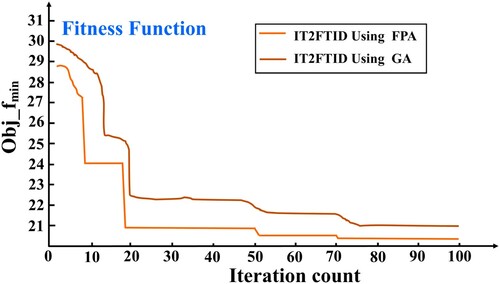
7.2. Performance of FPA

The expected PID controller tuning parameters are determined by application of optimization using FPA with sampling time 0.02 sec. The problem of optimization is treated as minimization of the objective function as characterized in Equation (28(28) ${\tilde{A}}_e={\int }_{x\in X}\left[1/u\right]/x,u\in J_x$(28) ). The Simulink model of the TTCNILS system with global variables of IT2-FTID and IT2-FPID controller as $K_p$, $K_i$, $K_d$, n, ${\text{β}}_1$ and ${\text{β}}_2$ is incorporated in MATLAB R2015b as shown in Figure 1. The IAE- and ITAE-based objective function as in Equation (28(28) ${\tilde{A}}_e={\int }_{x\in X}\left[1/u\right]/x,u\in J_x$(28) ), with global variables is written in ${}^{\ast }.\mathrm{m}$ file in MATLAB [55]. The upper and lower bound to the IT2-TID and IT2-PID parameters are set as shown in Equation (37(37) $\begin{array}{rl}& K_P^{min}\le K_P\le K_P^{max}\\ & K_I^{min}\le K_I\le K_I^{max}\\ & K_D^{min}\le K_D\le K_D^{max}\\ & n^{min}\le n\le n^{max}\\ & {\text{β}}_1^{min}\le {\text{β}}_1\le {\text{β}}_1^{max}\\ & {\text{β}}_2^{min}\le {\text{β}}_2\le {\text{β}}_2^{max}\end{array}$(37) ). The Number of population size to FPA are considered as 10 and the dimension is set to 3. The switch probability is considered as p=0.8 and the maximum number of iteration count is set as 100 for considering the termination of optimization. The performance of optimization in terms of fitness function value with iteration count is set at 100 and sampling time set as 0.02 second during optimization is shown in Figure 11. In [56] author presented the fault-tolerant control scheme using fuzzy logic for nonlinear level control process with intermittent fault and time delay constrain. The author of [57] proposed PID controller tuning using metaheuristic approach (ant colony optimization algorithm) and in [58] author use traditional zigler nichols (ZN) controller tuning method for tuning the parameters of the integer order PID and fractional order PID controller for conical two-tank (non-interacting) level control process with faults. In recent time, fuzzy harmonic search algorithm based optimization method of fuzzy controller is proposed for nonlinear systems and designed optimal fault-tolerant controller and found substantial statistical results under different uncertainties [59].

Figure 11. The behaviour of FPA & GA in terms of fitness function and iteration count.

(1) TTCNILS Response without Fault

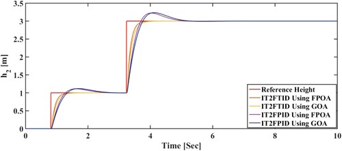
In Figure 9 TTCNILS system response without fault depicted, IT2-FTID and IT2-FPID controller comparative performance presented in Figure 12.

Figure 12. Simulated response of $\left(h_2\right)$ in TTCNILS without fault.

In the second phase of the simulation the proposed controller tested with two faults and process disturbances. The two faults consider in the TTCNILS system are system component (leak) and actuator, respectively, having abrupt in nature.

(2) TTCNILS Response with system component (leak) Fault

In Figure 13 TTCNILS system response with leak fault ($f_{\mathrm{s}\mathrm{y}\mathrm{s}}$ ) depicted, IT2-FTID and IT2-FPID controller comparative performance presented in Figure 13.

Figure 13. Simulated response of $\left(h_2\right)$ in TTCNILS with leak fault.

(3) TTCNILS Response with Actuator Fault

In Figure 14 TTCNILS system response with actuator fault ($f_a$) depicted, IT2-FTID and IT2-FPID controller comparative performance presented in Figure 14. From the result clearly represents that, the IT2FTID outperform the IT2FPID in terms of transient and steady-state performance.

Figure 14. Simulated response of $\left(h_2\right)$ in TTCNILS with actuator fault.

(4) TTCNILS Response with Process disturbances

In Figure 15 TTCNILS system response to process disturbances (d) depicted, IT2-FTID and IT2-FPID controller comparative performance presented in Figure 15.

Figure 15. Simulated response of $h_2$ in TTCNILS with uncertain process disturbances.

IT2FTID controller gives smooth steady-state response as compared to the IT2FPID controller because of FTID controller having four tuning parameters such as $K_P$, $K_I$, $K_D$, and n so more flexibility is there to tune the parameters.

Figures 16 and 17 illustrate the best fuzzy controller surface for IT2FTID and IT2FPID controller.

Figure 16. Fuzzy control surface for IT2FPID method for the TTCNILS [50].

Figure 17. Fuzzy control surface for IT2FTID method for the TTCNILS [50].

The superiority of the IT2FTID using FPA as compared to IT2FTID using GA measured with three errors (MAE, MSE and RMSE) which are presented in Figures 18 and  19.

Figure 18. Comparison of IT2FTID and IT2FPID controllers using FPA performance based on MAE/MSE/RMSE error.

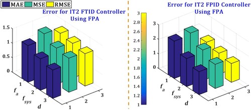
Figure 19. Comparison of IT2FTID and IT2FPID controllers using GA performance based on MAE/MSE/RMSE error.

7.2.1. Two-tank conical frustum non-interacting level control (TTCFNLC) process

In the second phase of the simulation the proposed controller tested with TTCFNLC process with two faults and uncertain process disturbances. The two faults consider in the TTCFNLC system are system component (leak) and actuator, respectively, having abrupt in nature.The magnitude and the nature of the fault are same which are consider for the TTCNILS process, the each fault magnitude value is 40% and the process disturbances magnitude is 40%. The time behaviour of all uncertainties is abrupt.

Fault scenarios in TTCFNLC

1. Actuator fault $\left(f_a\right)$

   • The actuator fault will be induced by $\left(\alpha \right)$, which denotes a faulty primary actuator (loss of efficacy) that regulates the regulated variable input flow rate $\left(f_{i}n\right)$. Equations (19(19) $\frac{\mathrm{d}{\mathrm{h}}_1}{\mathrm{d}\mathrm{t}}=\frac{(\alpha \times f_{in1})-f_{o1}-f_{12}}{\frac{\pi }{3}[3r_{b1}^2+6r_{b1}\left(\frac{R-r_{b1}}{H_1}\right)h_1+3{\left(\frac{R-r_{b1}}{H_1}\right)}^2{h_1}^2]}$(19) ) and (20(20) $\frac{\mathrm{d}{\mathrm{h}}_2}{\mathrm{d}\mathrm{t}}=\frac{f_{12}-(d\times f_{o2})-f_{out}}{\frac{\pi }{3}[3r_{b2}^2+6r_{b2}\left(\frac{R-r_{b2}}{H_2}\right)h_2+3{\left(\frac{R-r_{b2}}{H_2}\right)}^2{h}_2^2]}$(20) ) depict a broken system model with unknown parameters (actuator $\left(f_a\right)$ fault). The actuator fault into the TTCFNLC is introduce by changing the control output signal (u) positive or negative values can be taken as per fault requirement. The actuator fault in control valve $\left(f_a\right)$ magnitude $M=40\mathrm{\%}$.

2. System component fault $\left(f_{\mathrm{s}\mathrm{y}\mathrm{s}}\right)$

   • The system component fault (leak) introduce into conical frustum tank 2, the leak flow $f_{\mathrm{s}\mathrm{y}\mathrm{s}}=f_{o2}={\text{β}}_2{a}_2\sqrt{2g{h}_2}$ , where ${\text{β}}_2$ is valve coefficient for leak fault, $h_l$ is leak flow height and $\left(f_{\mathrm{s}\mathrm{y}\mathrm{s}}\right)$ is leak flow rate. The system component (leak) fault in conical frustum tank 2 $\left(f_{\mathrm{s}\mathrm{y}\mathrm{s}}\right)$ magnitude M= 40%.

Process disturbances in TTCFNLC

1. Process disturbances (d)

   • The process disturbances (d) introduces into TTCFNLC by adding step/ramp signal at particular time interval. The uncertain process disturbances magnitude M= 40%.

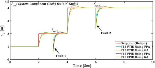
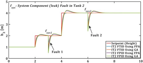
(1) TTCFNLC Response with system component (leak) Fault

In Figure 20 TTCFNLC system response with leak fault ($f_{\mathrm{s}\mathrm{y}\mathrm{s}}$ ) depicted, IT2-FTID and IT2-FPID controller comparative performance presented in Figure 20.

Figure 20. Simulated response of $\left(h_2\right)$ in TTCFNLC with leak fault.

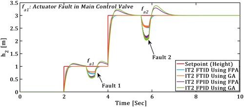
(2) TTCFNLC response with actuator fault

In Figure 21 TTCFNLC system response with actuator fault ($f_a$) depicted, IT2-FTID and IT2-FPID controller comparative performance presented in Figure 21. From the result clearly represents that, the IT2FTID outperform the IT2FPID in terms of transient and steady-state performance.

Figure 21. Simulated response of $\left(h_2\right)$ in TTCFNLC with actuator fault.

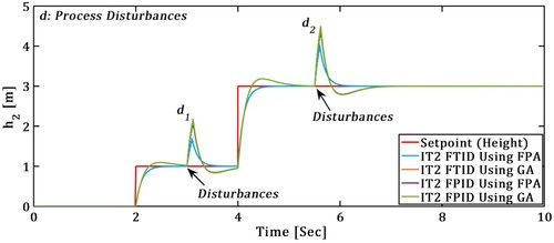
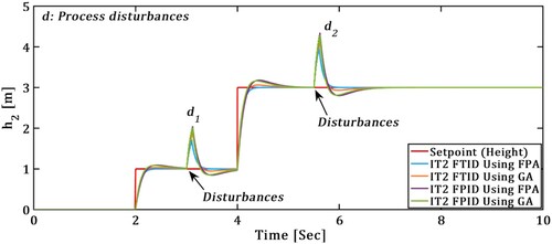
(3) TTCFNLC response with process disturbances

In Figure 22 TTCFNLC system response to process disturbances (d) depicted, IT2-FTID and IT2-FPID controller comparative performance presented in Figure 22.

Figure 22. Simulated response of $\left(h_2\right)$ in TTCFNLC with uncertain process disturbances.

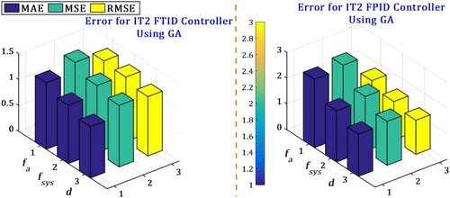
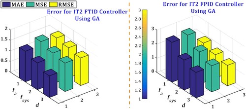
The superiority of the IT2FTID using FPA as compared to IT2FTID using GA measured with three errors (MAE, MSE and RMSE) which are presented in Figures 23 and 24.

Figure 23. Comparison of IT2FTID and IT2FPID controllers using FPA performance based on MAE/MSE/RMSE error.

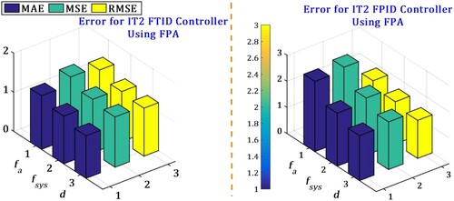
Figure 24. Comparison of IT2FTID and IT2FPID controllers using GA performance based on MAE/MSE/RMSE error.

7.3. Statistical test

To statistically verify the efficiency of the proposed method it was decided to use the z-test statistic, which is given by Equation (55(55) $Z=\frac{({\overline{X}}_1-{\overline{X}}_2)-({\mu }_1-{\mu }_2)}{{\sigma }_{{\overline{X}}_1-{\overline{X}}_2}}$(55) ), and the parameters used for the test are shown in Table 4: (55) $Z=\frac{({\overline{X}}_1-{\overline{X}}_2)-({\mu }_1-{\mu }_2)}{{\sigma }_{{\overline{X}}_1-{\overline{X}}_2}}$(55)

Table 4. Values for the statistical z-test.

Parameter	Value
Level of confidence	95%
Alpha	0.05
$H_a$	${\mu }_1<{\mu }_1$
$H_o$	${\mu }_1\ge {\mu }_1$
Critical value	−1.645

The alternative hypothesis indicates that the results of the IT2FTID method are smaller than the IT2FPID method and the null hypothesis indicates otherwise, with a rejection region for values lower than – 1.645.

Statistical results for TTCNILS

Based on the parameters of the z-test statistic presented in above subsection and Equation (55(55) $Z=\frac{({\overline{X}}_1-{\overline{X}}_2)-({\mu }_1-{\mu }_2)}{{\sigma }_{{\overline{X}}_1-{\overline{X}}_2}}$(55) ), the results of the Z-values are presented in Tables 5–10 for TTCNIL system subject to uncertainty (actuator fault, system component (leak) fault and process disturbances, respectively).

Table 5. Results for the statistical test of the TTCNILS subject to actuator $\left(f_a\right)$ fault using IT2FTID and IT2FPID with FPA.

RMSE	IT2FTID Using FPA	IT2FPID Using FPA
Best	8.256E-01	9.452E-01
Worst	10.048E-01	14.982E-01
Average	9.260E-01	12.232E-01
Standard deviation	6.89E-02	9.091E-02
Z-value	−16.061	−1.1256

Table 6. Results for the statistical test of the TTCNILS subject to system component (leak) $\left(f_{\mathrm{s}\mathrm{y}\mathrm{s}}\right)$ fault using IT2FTID and IT2FPID with FPA.

RMSE	IT2FTID Using FPA	IT2FPID Using FPA
Best	7.024E–01	8.189E–01
Worst	9.891E–01	12.045E–01
Average	8.363E–01	10.956E–01
Standard deviation	6.023E–02	8.789E–02
Z-value	−17.334	−1.1014

Table 7. Results for the statistical test of the TTCNILS subject to process disturbances (d) using IT2FTID and IT2FPID with FPA.

RMSE	IT2FTID Using FPA	IT2FPID Using FPA
Best	5.134E–01	6.098E–01
Worst	7.761E–01	10.125E–01
Average	6.723E–01	8.342E–01
Standard deviation	4.231E–02	6.124E–02
Z-value	−17.451	−1.0941

Table 8. Results for the statistical test of the TTCNILS subject to actuator $\left(f_a\right)$ fault using IT2FTID and IT2FPID with GA.

RMSE	IT2FTID Using GA	IT2FPID Using GA
Best	10.281E–01	11.564E–01
Worst	13.041E–01	15.012E–01
Average	10.279E–01	13.034E–01
Standard deviation	7.16E–02	9.991E–02
Z-value	−12.032	−1.318

Table 9. Results for the statistical test of the TTCNILS subject to system component (leak) $\left(f_{\mathrm{s}\mathrm{y}\mathrm{s}}\right)$ fault using IT2FTID and IT2FPID with GA.

RMSE	IT2FTID Using GA	IT2FPID Using GA
Best	9.016E–01	10.434E–01
Worst	12.012E–01	14.108E–01
Average	9.114E–01	12.201E–1
Standard deviation	6.0148E–02	8.891E–02
Z-value	−13.561	−1.3561

Statistical results for TTCFNLC

Based on the parameters of the z-test statistic presented in above subsection and Equation (55(55) $Z=\frac{({\overline{X}}_1-{\overline{X}}_2)-({\mu }_1-{\mu }_2)}{{\sigma }_{{\overline{X}}_1-{\overline{X}}_2}}$(55) ), the results of the Z-values are presented in Tables 11–16 for TTCFNLC system subject to uncertainty (actuator fault, system component (leak) fault and process disturbances, respectively).

Table 11. Results for the statistical test of the TTCFNLC subject to actuator $\left(f_a\right)$ fault using IT2FTID and IT2FPID with FPA.

RMSE	IT2FTID Using FPA	IT2FPID Using FPA
Best	9.768E–01	11.0821E–01
Worst	11.491E–01	15.567E–01
Average	10.745E–01	13.765E–01
Standard deviation	7.983E–02	10.193E–02
Z-value	−15.823	−1.0127

Table 10. Results for the statistical test of the TTCNILS subject to process disturbances (d) using IT2FTID and IT2FPID with GA.

RMSE	IT2FTID Using GA	IT2FPID Using GA
Best	7.106E–01	8.564E–01
Worst	10.127E–01	12.086E–01
Average	7.118E–01	10.301E–1
Standard deviation	4.1235E–02	6.671E–02
Z-value	−13.897	−1.391

Table 12. Results for the statistical test of the TTCFNLC subject to system component (leak) $\left(f_{\mathrm{s}\mathrm{y}\mathrm{s}}\right)$ fault using IT2FTID and IT2FPID with FPA.

RMSE	IT2FTID Using FPA	IT2FPID Using FPA
Best	8.658E–01	10.121E–01
Worst	10.341E–01	14.367E–01
Average	9.675E–01	12.605E–01
Standard deviation	6.783E–02	9.093E–02
Z-value	−16.478	−1.009

Table 13. Results for the statistical test of the TTCFNLC subject to process disturbances (d) using IT2FTID and IT2FPID with FPA.

RMSE	IT2FTID Using FPA	IT2FPID Using FPA
Best	6.438E–01	8.107E–01
Worst	8.121E–01	12.217E–01
Average	7.465E–01	10.554E–01
Standard deviation	4.413E–02	5.183E–02
Z-value	−16.643	−1.114

Table 14. Results for the statistical test of the TTCFNLC subject to actuator $\left(f_a\right)$ fault using IT2FTID and IT2FPID with GA.

RMSE	IT2FTID Using FPA	IT2FPID Using FPA
Best	12.312E–01	13.678E–01
Worst	15.245E–01	17.167E–01
Average	12.342E–01	15.108E–01
Standard deviation	9.378E–02	12.013E–02
Z-value	−11.871	−1.387

Table 15. Results for the statistical test of the TTCFNLC subject to system component (leak) $\left(f_{\mathrm{s}\mathrm{y}\mathrm{s}}\right)$ fault using IT2FTID and IT2FPID with GA.

RMSE	IT2FTID Using FPA	IT2FPID Using FPA
Best	11.282E–01	12.638E–01
Worst	14.105E–01	16.107E–01
Average	11.182E–01	14.218E–01
Standard deviation	8.118E–02	11.134E–02
Z-value	−12.783	−1.276

From the statistical results, we can surly say that the proposed control approach IT2FTID using FPA is Superior for bot the uncertain level control process under various uncertainties.

Table 16. Results for the statistical test of the TTCFNLC subject to process disturbances (d) using IT2FTID and IT2FPID with GA.

RMSE	IT2FTID Using FPA	IT2FPID Using FPA
Best	9.197E–01	11.578E–01
Worst	13.203E–01	15.0947E–01
Average	10.082E–01	13.157E–01
Standard deviation	7.089E–02	10.115E–02
Z-value	−13.0923	−1.291

The Z-values obtained for the statistical test demonstrate the improvement of the proposed IT2FTID approach with respect to the IT2FPID method with two different metaheuristic algorithms.

Critical Observations

• When compared to system component (leak) faults, the actuator fault degrades TTCNILS and TTCFNLC performance significantly.

• The proposed controller is validated by the abrupt nature of the actuator and the leak fault it introduces. TTCNILS and TTCFNLC, on the other hand, did not take into account the incipient form of the two faults.

• Out of three possible faults in TTCNILS and TTCFNLC two major faults introduced into the system.

• In comparison to traditional PID controllers, fractional order FOPID controllers are more flexible in terms of tuning parameters, allowing for fine tuning.

• The key reason for using the Flower Pollination Optimization Algorithm (FPA) to optimize the controller parameters is because it has few parameters and is simple to implement, requiring less processing.

• For TTCNILS and TTCFNLC, the FPA-based IT2FTID and IT2FPID controllers will provide optimum and superior response when compared to GA-based IT2FTID and IT2FPID controllers, subject to three uncertainties.

8. Conclusions

The use of the flower pollination algorithm (FPA) to design an optimal IT2FTID/IT2FPID controller for two nonlinear uncertain level control systems with two faults and process disturbances is proposed in this study. In this paper, the two-tank conical and two-tank frustum conical, non-interacting level system (TTCNILS) and (TTCFNLC) systems were investigated as real-world second-order systems (SOS) that are commonly required in industries.The FPA, one of the most effective population-based metaheuristic optimization approaches, was used, which is based on current optimization. Furthermore, for the proposed nonlinear system, two controller optimizations were performed using two different metaheuristic optimization methods, FPA and GA, and comparative simulation results were displayed using statistical analysis. Also offered is a fault recovery time analysis to test the effectiveness of the suggested controller in a faulty circumstance. Simulation results reveal that the FPA's IT2FTID controller can offer a more satisfying response than the TTCNILS and TTCFNLC control system's IT2FPID controller when subjected to modelling uncertainty, errors, and process disruptions. A metaheuristic approach for highly nonlinear and stochastic systems can be used to optimize fuzzy fault-tolerant control in the future..

Author contributions

Conceptualization, H.R.P.; methodology, H.R.P.; software, H.R.P.; validation, H.R.P.; formal analysis, H.R.P.; investigation, H.R.P.; resources, H.R.P., and V.A.S.;data curation, H.R.P.; writing-original draft preparation, H.R.P.; writing-review and editing, H.R.P. and V.A.S.; supervision V.A.S.; All authors have read and agreed to the published version of the manuscript.

Acknowledgments

The project outcome is Ph.D work of corresponding author of this article. This research received no external funding.The authors would also like to thank Department of Instrumentation and Control, Faculty of Technology, Dharmsinh Desai University, Nadiad-387001, Gujarat, India.

Disclosure statement

No potential conflict of interest was reported by the author(s).

Additional information

Funding

This research received no specific grant from any funding agency in the public, commercial, or not-for-profit sectors.

References

- Pannu HS, Singh D, Malhi AK. Improved particle swarm optimization based adaptive neuro-fuzzy inference system for benzene detection. CLEAN-Soil Air Water. 2018;46(5):1700162. Article ID. DOI: https://doi.org/10.1002/clen.201700162
- Yang XS. Flower pollination algorithm for global optimization. Unconventional computation and natural computation. 2012. p. 240–249. (Lecture Notes in Computer Science; 7445).
- Himanshukumar RP, Vipul AS. Actuator and system component fault tolerant control using interval type-2 Takagi-Sugeno fuzzy controller for hybrid nonlinear process. Int J Hybrid Intell Syst. 2019;15(3):143–153.
- Himanshukumar RP, Vipul AS. A fault-tolerant control strategy for non-linear system: an application to the two tank canonical noninteracting level control system. IEEE Distributed Computing, VLSI, Electrical Circuits and Robotics (DISCOVER-2018); Mangalore (Mangaluru), India, 13–14 Aug 2018. p. 64–70.
- Himanshukumar RP, Vipul AS. A passive fault-tolerant control strategy for a non-linear system: an application to the two tank conical non-interacting level control system. MASKAY. 2019;9(1):1–8. DOI: https://doi.org/10.24133/maskay.v9i1.1094.
- Himanshukumar RP, Vipul AS. A framework for fault-tolerant control for an interacting and non-interacting level control system using AI. In Proceedings of the 15th International Conference on Informatics in Control, Automation and Robotics – Volume 1: ICINCO; p. 180–190. ISBN 978-989-758-321-6.
- Himanshukumar RP, Vipul AS. Fuzzy logic based passive fault tolerant control strategy for a single-tank system with system fault and process disturbances. 5th International Conference on Electrical and Electronic Engineering (ICEEE-2018); Istanbul: 2018, p. 257–262.
- Mohammad S. PID control for Industrial processes. London: IntechOpen; 2018. DOI: https://doi.org/10.5772/intechopen.69592.
- Kadu CB, Patil CY. Design and implementation of stable PID controller for interacting level control system. Procedia Comput Sci. 2016;79:737–746.
- Prusty S, Pati UC, Mahapatra K. Implementation of fuzzy-PID controller to liquid level system using LabVIEW. International Conference on Control, Instrumentation, Energy and Communication, (CIEC 2014); p. 36–40.
- Himanshukumar RP, Vipul AS. Passive fault tolerant control system using feed-forward neural network for two-Tank interacting conical level control system against partial actuator failures and disturbances. IFAC–PapersOnLine. 2019;52(14):141–146.
- Himanshukumar RP, Vipul AS. Fault tolerant control systems: a passive approaches for single tank level control system, i-manager's. J Instrumentation Control Eng. 2018;6(1):11–18.
- Bhawna T, Randeep K. Genetic algorithm based parameter tuning of PID controller for composition control system. Int J Eng Sci Technol. 2011;3(8):6705–6711.
- Anju KV, Ruban N. Particle swarm optimization based PID controller tuning for level control of two tank system. 14h ICSET-2017, IOP Conf. Series: Materials Science and Engineering; Vol. 263, 2017. p. 1–7.
- Latha K, Rajinikanth V, Surekha PM. PSO-Based PID controller design for a class of stable and unstable systems. ISRN Artificial Intelligence. 2013;543607:00–Article ID.
- Himanshukumar RP, Vipul AS. Fault tolerant controller using interval type-2 TSK logic control systems: application to three interconnected conical tank system. In: Kearfott R, Batyrshin I, Reformat M, editors. Fuzzy techniques: theory and applications. IFSA/NAFIPS 2019. Cham: Springer; 2019. (Advances in Intelligent Systems and Computing; 1000).
- Himanshukumar RP, Vipul AS. Fault tolerant control using interval type-2 Takagi-Sugeno fuzzy controller for nonlinear system. In: Abraham A, Cherukuri A, Melin P, editors. Intelligent systems design and applications. ISDA 2018. Cham: Springer; 2018. (Advances in Intelligent Systems and Computing; 941).
- Patel HR, Raval SK, Shah VA. A novel design of optimal intelligent fuzzy TID controller employing GA for nonlinear level control problem subject to actuator and system component fault. Int J Intell Comput Cybern. 2021;14(1):17–32.
- Patel HR, Shah VA. Stable fuzzy controllers via LMI approach for non-linear systems described by type-2 T-S fuzzy model. Int J Intell Comput Cybern. 2021;14(3):509–531.
- Himanshukumar RP, Vipul AS. Fault detection and diagnosis methods in power generation plants – the Indian power generation sector perspective: an introductory review. J Energy Manag. 2018;2:31–39.
- Lurie BJ. Three-parameter tunable tilt-integral-derivative (TID) Controller. United States Patent; 1994.
- Himanshukumar RP, Vipul AS. An optimized intelligent fuzzy fractional order TID controller for uncertain level control process with actuator and system component uncertainty. In: Bede B, Ceberio M, De Cock M, editiors. Fuzzy information processing 2020. NAFIPS 2020. Cham: Springer; 2022. p. 183–195. (Advances in Intelligent Systems and Computing; 1337). DOI: https://doi.org/10.1007/978-3-030-81561-5_16.
- Himanshukumar RP, Vipul AS. Comparative study of interval type-2 and type-1 fuzzy genetic and flower pollination algorithms in optimization of fuzzy fractional order PIλDμ controllers. Intelligent system and computing, Yang (Cindy) Yi. (January 3rd 2020). IntechOpen. DOI: https://doi.org/10.5772/intechopen.90359.
- Lakshmanaprabu SK, Nasir AV, BanuSabura U. Design of centralized fractional order PI controller for two interacting conical frustum tank level process. J Appl Fluid Mech. 2017;10:23–32.
- Garcia D, Karimi A, Longchamp R. PID controller design for multivariable systems using Gershgorin bands. IFAC Proc. 2005;38(1):183–188.
- Dittmar R, Gill S, Singh H, et al. Robust optimization-based multi-loop PID controller tuning: a new tool and its industrial application. Control Eng Pract. 2012 Apr;20(4):355–370.
- Euzébio TAM, Barros PR. Iterative procedure for tuning decentralized PID controllers. IFAC-PapersOnLine. 2015;48(8):1180–1185.
- Naik RH, Kumar DVA, Rao PVG. Improved centralised control system for rejection of loop interaction in coupled tank system. Indian Chem Eng. 2020;62(2):118–137.
- Lakshmanaprabu SK, Elhoseny M, Shankar K. Optimal tuning of decentralized fractional order PID controllers for TITO process using equivalent transfer function. Cogn Syst Res. 2019 Dec;58:292–303.
- Aparna V, Hussain K. M, Jamal DN, et al. Implementation of gain scheduling multiloop PI controller using optimization algorithms for a dual interacting conical tank process. Proc. 2nd Int. Conf. Trends Electron. Informat. (ICOEI); 2018 May. p. 598–603.
- Euzébio TAM, Silva MTD, Yamashita AS. Decentralized PID controller tuning based on nonlinear optimization to minimize the disturbance effects in coupled loops. IEEE Access. 2021;9:156857–156867.
- Euzébio TA, Yamashita AS, Pinto TV, et al. SISO approaches for linear programming based methods for tuning decentralized PID controllers. J Process Control. 2020;94:75–96.
- Nadweh S, Khaddam O, Hayek G, et al. Optimization of P & PI controller parameters for variable speed drive systems using a flower pollination algorithm. Heliyon. 2020;6:e04648–
- Nayak PSR, Rufzal TA. Flower pollination algorithm based PI controller design for induction motor scheme of soft-Starting. 2018 20th National Power Systems Conference (NPSC); 2018. p. 1–6.
- Castelo Damasceno N, Gabriel Filho O. PI controller optimization for a heat exchanger through metaheuristic bat algorithm, particle swarm optimization, flower pollination algorithm and Cuckoo search algorithm. IEEE Latin America Trans. 2017;15:1801–1807.
- Himanshukumar RP, Vipul AS. A novel design of centralized fractional order PID controller and its optimal time domain tuning: a hybrid two interacting conical frustum tank level process case study. Memorias del Congreso Nacional de Control Autom Atico (CNCA 2019); Puebla, Mexico 23–25 de octubre de 2019. p. 754–761, ISBN 2594–2492.
- Himanshukumar RP, Vipul AS. A fractional and integer order PID controller for nonlinear system: two non-interacting conical tank process case study. In: Mehta A, Rawat A, Chauhan P, editors. Advances in control systems and its infrastructure. Singapore: Springer; p. 37–55. (Lecture Notes in Electrical Engineering; 604).
- Himanshukumar RP, Vipul AS. General type-2 fuzzy logic systems using shadowed sets: a new paradigm towards fault-tolerant control. 2021 Australian & New Zealand Control Conference (ANZCC); 2021. p. 116–121.
- Himanshukumar RP., Vipul AS. Stable fault tolerant controller design for Takagi-Sugeno fuzzy model-Based control systems via linear matrix inequalities: three conical tank case study. Energies. 2019;12(11):2221.
- Maalej I, Abid DBH, Rekik C. Active fault tolerant control design for stochastic interval type-2 Takagi-Sugeno fuzzy model. Int J Intell Comput Cybern. 2018;11(3):404–422.
- Mendel JM, John RI, Liu F. Interval type-2 fuzzy logic systems made simple. IEEE Trans Fuzzy Syst. 2006;14:808–821.
- Mendel JM, Hagras H, John RI. Standard background material about interval type-2 fuzzy logic systems that can be used by all authors. IEEE Comput Intell Soc. 2010;1–11.
- H Hagras. A hierarchical type-2 fuzzy logic control architecture for autonomous mobile robots. IEEE Trans Fuzzy Syst. 2004;12:524–539.
- Wu H, Mendel IM. Uncertainty bounds and their use in the design of interval type-2 fuzzy logic systems. IEEE Trans Fuzzy Syst. 2002;10(5):622–639.
- Glover BJ. Understanding flowers and flowering: an integrated approach. Oxford: Oxford University Press; 2007. DOI: https://doi.org/10.1093/acprof:oso/9780198565970.001.0001.
- Willmer P. Pollination and floral ecology. Princeton, NJ: Princeton University Press; 2011.
- Balasubramani K, Marcus K. A study on flower pollination algorithm and its applications. Int J Appl Innov Eng Manag (IJAIEM). 2014;3:320–325.
- Abdel-Raouf O, Abdel-Baset M. A new hybrid flower pollination algorithm for solving constrained global optimization problems. Int J Appl Oper Res-An Open Access J. 2014;4(2):1–13.
- Man KF, Tang KS, Kwong S. Genetic algorithms: concepts and applications. IEEE Trans Indust Electron. 1996;43(5):519–534. [cited: 2018 Aug 2].
- Fevrier V, Patricia M, Oscar C. Fuzzy logic for parameter tuning in evolutionary computation and bio-inspired methods, Berlin Heidelberg: Springer-Verlag; 2010. 465–474. (LNAI; 1648) [cited 2018 Aug 22].
- Bernd F, Michael H. Optimization of genetic algorithms by genetic algorithms. Artificial neural nets and genetic algorithms. Vienna: Springer; 1993. [cited 2018 Aug 28].
- Kumbasar T, Hagras H. Big bang-big crunch optimization based interval type-2 fuzzy PID cascade controller design strategy. Inf Sci. 2014;282:277–295.
- Sambariya DK, Gupta T. Optimal design of PID controller for an AVR system using monarch butterfly optimization. 2017 International Conference on Information, Communication, Instrumentation and Control (ICICIC); 2017. p. 1–6.
- Taskin A, Kumbasar T. An open source matlab/simulink tool box for interval type-2 fuzzy logic systems. 2015 IEEE Symp Ser Comput Intell; 2015. p. 1561–1580.
- Mendel JM. Rule-Based fuzzy logic systems: introduction end new directions. NI: Prentice-Hall; 2001.
- Himanshukumar RP, Vipul AS. Passive fault–Tolerant tracking for nonlinear system with intermittent fault and time delay. IFAC–PapersOnLine. 2019;52(11):200–205.
- Latha K, Rajinikanth V, Surekha PM. Application of ant colony optimization in tuning a PID controller to a conical tank. Indian J Sci Technol. 2015;8(S2):217.
- Himanshukumar RP, Vipul AS. Comparative study between fractional order PIλDμ and integer order PID controller: a case study of coupled conical tank system with actuator faults. 2019 4th Conference on Control and Fault Tolerant Systems (SysTol); Casablanca, Morocco: 2019. p. 390–396.
- Patel Himanshukumar Rajendrabhai. Fuzzy-based metaheuristic algorithm for optimization of fuzzy controller: fault-tolerant control application. International Journal of Intelligent Computing and Cybernetics. 2022;13:93), https://doi.org/https://doi.org/10.1108/IJICC-09-2021-0204.