Dissipation Element Analysis of Turbulent Premixed Jet Flames

ABSTRACT

Dissipation element (DE) analysis is a method for analyzing scalar fields in turbulent flows. DEs are defined as a coherent region in which all gradient trajectories of a scalar field reach the same extremal points. Therefore, the scalar field can be compartmentalized in monotonous space-filling regions.

The DE analysis is applied to a set of spatially evolving premixed jet flames at different Reynolds numbers. The simulations feature finite rate chemistry with 16 species and 73 reactions. The jet consists of a methane/air mixture with an equivalence ratio φ = 0.7.

Statistics of DE parameters are shown and compared to those of a DNS of a non-reacting spatial jet, a non-reacting temporally evolving jet and isotropic homogeneous turbulence.

The invariance of the normalized length distribution of the DEs toward changes in Reynolds number observed in non-reacting flows holds for the reacting cases and the characteristic scaling with Kolmogorov micro-scale is reproduced. Furthermore, the DE statistics reflect the influence of the premixed flame structure on the turbulent scalar fields.

KEYWORDS:

• Premixed flames
• turbulent combustion
• direct numerical simulation
• isotropic turbulence

Introduction

In turbulent flames, various combustion regimes exist which pose different implications to the accompanying modeling procedure. For premixed combustion, the so-called “Borghi-Peters-diagram” can be constructed (Peters, 2000). Turbulent scales, such as the Kolmogorov length, are compared to different scales of the flame. To test the underlying theory of the combustion diagram by means of direct numerical simulations (DNS), a set of simulations of spatially evolving jet flames situated in the thin reaction zone regime was employed by (Luca, S., Attili, A. et al., 2019). To achieve a meaningful comparison between the local turbulent and chemical scales, a procedure employing a space-filling decomposition to assure that all interactions are being considered is required. A method for obtaining the local turbulent scales in a turbulent scalar field is the dissipation element (DE) analysis (Peters and Wang, 2006; Wang and Peters, 2006, 2008). DEs are constructed by tracing gradient trajectories in a scalar field in the ascending direction until a maximum is reached and in the descending direction until the gradient trajectory terminates at a local minimum. All grid points whose gradient trajectories reach the same extremal points are grouped into a single DE. DEs can be described by two parameters, namely the Euclidean distance between their extremal points ℓ and the scalar difference in these points $\mathrm{\Delta }\varphi$. The joint probability density function (jPDF) of these two parameters is expected to suffice for a statistical reconstruction of the scalar field.

DE analysis was originally applied to scalar fields in isotropic turbulence (Peters and Wang, 2006; Wang and Peters, 2006, 2008), later to free shear flows (Gampert et al., 2011; Gampert, Schäfer, et al., 2013a) and verified in experiments (Gampert et al., 2013c; Gampert et al., 2014). More recently, the DE analysis was applied to a non-premixed jet flame (Gauding et al., 2017; Scholtissek et al., 2017).

Additionally, marginal and joint statistics of normalized DE parameters can be modeled by employing stochastic transport equations developed originally for isotropic turbulence (Wang and Peters, 2008). In the context of turbulent reacting flows, DE statistics were successfully used to model the intermittency of the temperature field in the computational fluid dynamics of a gasoline engine (Peters et al., 2013).

In this work, the DE analysis is applied to the temperature fields of two premixed flame DNS whose details will be outlined in the section below. Since the temperature can be interpreted as a progress variable in the context of premixed combustion, the gradient trajectories used in forming a DE can be interpreted as a grouping of flamelets, which share the same start and end points in space. To investigate the difference of the turbulent scales obtained from scalar fields of reacting and non-reacting flows, the DE analysis is additionally applied to passive scalar fields of a spatially evolving jet and isotropic homogeneous turbulence.

Configurations

The DE analysis was applied to two DNS of spatially evolving methane jet flames in the Bunsen burner configuration. An outline of the flames is illustrated in Figure 1, where the atomic oxygen mass fraction in the x-y center plane of the two reacting DNS is shown.

Figure 1. Atomic oxygen mass fraction in the x-y center plane of the two DNS cases investigated here. The yellow colored regions correspond to high values of the mass fraction, and brown colored regions to low values.

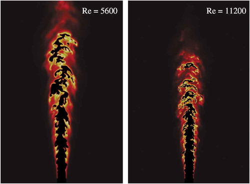
The jet Reynolds number is set to 5,600 and 11,200 for the Low Re Flame and the high Re case, respectively. The jet Reynolds number is varied by changing the slot width H while keeping the jet bulk velocity constant. In this fashion, the small scales of turbulence remain approximately constant while the integral scales are changed.

The DNS feature lean premixed methane/air flames with an equivalence ratio of φ = 0.7 and a temperature of the unburned mixture of ${\mathrm{T}}_{\mathrm{u}}=800K$, as it is commonly found in stationary gas turbines. The temperature and species concentrations in the co-flow correspond to the equilibrium state of the burned mixture.

The laminar burning velocity is s_L = 1.01 ms⁻¹ and the temperature-gradient-based laminar flame thickness is δ_L = 110 μm. The DNS is performed in the low Mach number limit using finite rate chemistry with a skeletal mechanism with 16 species and 73 elementary reactions (Luca et al., 2018). Additional details regarding the spatially evolving DNS are summarized in Table 1. The reacting cases are statistically homogeneous in the span-wise z direction and inhomogeneous in the stream-wise x and cross-stream y direction. The flame behavior is fully consistent with the “thin reaction zones” regime, with turbulent mixing influencing the pre-heating zone for $T<1800K$ and limited influence for temperatures above this value. Further information on the configuration and the methods employed in the DNS can be found in Luca, S., Attili, A. et al., (2019).

Table 1. Summary of the details of the DNS investigated with the DE analysis.

	Low Re Flame	Inert Spatially Evolving case	High Re Flame	Inert Temporally Evolving case	Inert Isotropic case
Jet Reynolds number Re	5,600	5,600	11,200	9,850	-
Jet bulk velocity U	100 ms^−1	100 ms^−1	100 ms^−1	1	-
Slot with H	1.2 mm	1.2 mm	2.4 mm	1	-
Karlovitz number Ka	23	-	21	-	-
Grid size (nx × ny × nz)	1440 × 960 × 256	1440 × 960 × 256	2880 × 1920 × 512	2560 × 2560 × 1312	512 × 512 × 512

The Bunsen burner configuration possesses several fundamental differences to the isotropic turbulence, on which the DE analysis was most extensively applied and for which the underlying theory was developed. To isolate effects on the DE parameter statistics, three additional non-reactive DNS cases are included in this study.

To investigate the difference between the turbulent scalar fields in a reacting and a non-reacting flow, a DNS using the exact configuration and inflow velocity field of the Low Re Flame was conducted omitting the combustion and using the homogeneous material properties of the unburned lean premixed air/methane mixture. A passive scalar was added with boundary conditions of $\varphi =1$ in the slot and $\varphi =0$ in the co-flow. The Schmidt number of the passive scalar is set to $S_c=1$. This DNS is henceforth called the Inert Spatially Evolving case and additional information is given in Table 1.

To identify the effects of the spatially evolving nature of the previously outlined cases on the scalar fields, DNS data of a temporally evolving non-reacting jet, referred to as the Inert Temporally Evolving case, are included in this investigation. The non-dimensional DNS features a comparable Jet Reynolds number to the High Re Flame of ${Re}_{\mathrm{j}\mathrm{e}\mathrm{t}}=9,850$. The flow and the scalar fields are statistically homogeneous in the stream-wise direction x and span-wise direction y. The non-dimensional size of the domain is $L_x=6\pi$, $L_y=6\pi$, and $L_z=12.5$, discretized by 2560 × 2560 × 1312 grid points. The initial mean velocity profile was initialized as two mirrored hyperbolic-tangent profiles. Uncorrelated velocity fluctuations with an intensity of 5% were superimposed onto the mean profile around the shear layer and damped toward the center plane and the outer region. The mean scalar profiles were initialized in the same way of the mean velocity profile, but non-perturbed. The passive scalar with a unity Schmidt number at the non-dimensional time instant t = 23 is used for the following investigation. At this instant, the jet is in a fully turbulent and self-similar state. For additional details regarding the numerical approach, the reader is referred to (Hunger et al., 2016).

As a final point of reference for the analysis, a passive scalar field of a DNS of forced isotropic turbulence with a Taylor-based Reynolds number of ${Re}_{\lambda }=88$ is used, which is similar to those of the High Re Flame and the Inert Temporally evolving case. The computational domain is a box with periodic boundary conditions and a non-dimensional length of $2\pi$. The domain is discretized with 512³ grid points. Statistical steadiness is ensured via the stochastic forcing scheme. Again, the subsequent investigation is based on a passive scalar with a unity Schmidt number. Additional information can be found in Gauding (2014). This case will be referred to as the Inert Isotropic case in the following sections.

Marginal statistics dissipation element parameter

The DE analysis is applied to the temperature fields of the reacting DNS in two different stream-wise regions. This is necessary as statistics are bound to change as the flow is traversed in the stream-wise direction. The upstream region corresponds to a stream-wise region of $x\approx 0.27L_F$ to $x\approx 0.54L_F$, where $L_F$ is the mean flame length. In this region, the turbulence is already sufficiently evolved for a DE analysis. Here, the two flame fronts are approximately parallel. The second region, henceforth called the downstream region, is situated at $x\approx 0.54L_F-0.81L_F$, where the flame fronts show the first signs of closing in on themselves. These two stream-wise regions are also chosen for the DE analysis of the passive scalar in the Inert Spatially Evolving case to achieve a meaningful comparison of the statistics in the spatially evolving cases. In both the Inert Temporally evolving case and the Inert Isotropic case, the entire passive scalar fields were subjected to DE analyses. In the free shear flow cases, DEs whose extremal points are located in the irrotational regions of the flows were omitted from the statistics. These regions were identified using the turbulent/non-turbulent interface criterion of (Bisset et al., 2002).

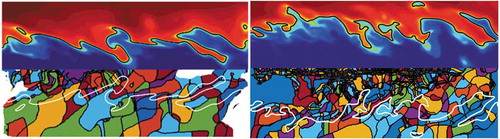
The DE analysis for the reacting cases is shown in Figure 2 for the x-y center plane of the temperature fields in the upstream region. On the top part of the figure, the temperature fields are shown as well as a black contour indicating the iso line of the temperature where the heat release peaks to mark the region of the flame front. On the bottom part of Figure 1, the DE analysis is shown in a mirrored fashion. The DEs are colored individually and encompassed in a black contour. For the sake of orientation, the iso-line of the temperature of the maximum heat release is again shown in white. One observes that, compared to the jet thickness in the cross-stream direction, the DEs of the High Re Flame are a lot smaller in scale than in the Low Re Flame. In addition, the various shapes and sizes of the DEs intersecting the flame front indicate a wide range of local turbulent scales interacting with the flame. The anisotropic nature of the scales becomes apparent when the spatial change in DE sizes is considered. In both cases, the DE sizes grow moving away from the jet core and approaching the flame front.

As a reference, the cross-section of the DE analysis of the passive scalar field in the Inert Isotropic case is shown in Figure 3. Again, the DEs are colored individually and encompassed in a black contour. One observes a wide range of sizes and shapes of the DEs similar to the ones previously beheld in the analysis of the jet flames in Figure 2. As expected, the isotropic nature of the scalar field carries over to the distribution of the DEs with no apparent preferential orientation of the DEs.

Figure 3. DE analysis of the passive scalar field in the Inert Isotropic case. The DE are colored individually and encompassed in a black contour.

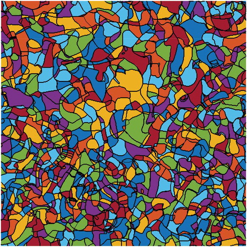
Figure 2. Top part: upstream x-y center plane of the temperature fields in two DNS of spatially evolving methane jet flames. The red colored regions correspond to high temperatures, blue color to low temperature regions. The black contour indicates the iso-surface of the maximum heat release. Bottom part: The mirrored corresponding DE analysis of the temperature. The DEs are colored individually and encompassed in a black contour. Left: Low Re Flame, right: High Re case.

These qualitative observations will be quantified in the following via statistics of the DE parameters. First, the volume averaged values of the DE parameters, the mean separation DE length ${\mathrm{\ell }}_m$, the mean DE scalar difference $\mathrm{\Delta }{\varphi }_{\mathrm{m}}$, or mean DE temperature difference $\mathrm{\Delta }{T}_{\mathrm{m}}$ for the reacting cases, will be investigated as they provide the means of normalization in the subsequent analysis. The mean separation length ${\mathrm{\ell }}_m$ normalized with the Kolmogorov micro-scale $\eta$ is shown in Figure 4(a) for all cases. The Kolmogorov scale is defined as $\eta ={\left(\frac{{\bar{\nu }}^3}{\tilde{\epsilon }}\right)}^{1/4}$, where $\tilde{\epsilon }$ is the Favre averaged energy dissipation and $\bar{\nu }=\frac{\bar{\mu }}{\rho }$ is the averaged viscosity. For the spatially evolving cases for each stream-wise region, the Kolmogorov scale for the normalization is computed at the lateral position corresponding to the center of the flame brush.

Figure 4. a): Normalized mean DE length ${\mathrm{\ell }}_{\mathrm{m}}/\eta$. b): Normalized mean DE differences Δϕ_m$\mathrm{\Delta }$ϕ_max and $\mathrm{\Delta }{T}_{\mathrm{m}}/\mathrm{\Delta }{T_{\mathrm{m}}}_{\mathrm{a}\mathrm{x}}$. The blue, red and green diamonds correspond to the Low Re Flame, High Re Flame and Inert Spatially Evolving case, respectively. The solid symbols indicate the upstream region; the hollow, black dashed symbols indicate the downstream region. The Inert Temporally Evolving case and the Inert Isotropic case are indicated by the solid purple triangle and black square, respectively. The abscissa position of the Inert Isotropic case was chosen arbitrarily, as no jet Reynolds number exists.

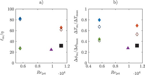
A scaling of ${\mathrm{\ell }}_m$ with $\eta$ was reported in (Wang, 2009; Gampert et al., 2013b), and this holds true for the Inert Spatially Evolving case analyzed here. Spanning a wide range of Reynolds numbers and three different flow configurations, the ratio of the two length scales comes to $l_{\mathrm{m}}/\eta \approx 30$, which is consistent with previous DE investigations of non-reacting flows. For the Inert Spatially Evolving case, ${\mathrm{\ell }}_{\mathrm{m}}/\eta$ collapses in both upstream and downstream regions. However, for the reacting cases, ${\mathrm{\ell }}_{\mathrm{m}}/\eta$ is approximately twice as large, indicating larger turbulent length scales in the temperature field as compared to the passive scalar field. The scaling with the Kolmogorov micro-scale is not as evident as in the inert cases with ${\mathrm{\ell }}_{\mathrm{m}}/\eta \approx 82$ for the Low Re Flame and ${\mathrm{\ell }}_{\mathrm{m}}/\eta \approx 62$ the High Re case. However, this could be attributed to the low Reynolds number in the Low Re Flame.

The higher values for ${\mathrm{\ell }}_{\mathrm{m}}/\eta$ can be attributed largely to two effects. The first effect is the dilatation resulting from the inherent different densities in the extremal points, not present in the passive scalar extremal points. The different densities cause a relative velocity between the extremal points, which counteracts the drift velocity of the extremal points. Assuming the lifetime of the DE in the Diffusive drift region to be of the order of the Kolmogorov time ${\tau }_{\eta }$, the dilatation causes ${\mathrm{\ell }}_{\mathrm{m}}$ to be enlarged significantly for the reactive cases, which display high values of $\mathrm{\Delta }{T}_{\mathrm{m}}$ and, therefore, a large difference in density. A second effect not present in the non-reactive cases is the non-unity Schmidt number $S_c=\frac{\nu }{D}\approx 0.7$ of the temperature fields in the reacting cases. To account for larger turbulent scales due to a higher diffusion coefficient, the Batchelor scale ${\lambda }_B=\eta {S_c}^{-0.5}$ might be a more suitable scaling length accounting for the larger normalized DE length, which would lead to an approximately 20% smaller ratio. Overall, with the inherent uncertainty left in estimating Kolmogorov scale and considering the vastly different configurations and range of Reynolds numbers the DE analysis is applied to, these results indicates that the Kolmogorov scaling of ${\mathrm{\ell }}_{\mathrm{m}}$ applies to reacting flows as well.

While there is only a slight difference of ${\mathrm{\ell }}_{\mathrm{m}}/\eta$ from the upstream to the downstream region for the Low Re Flame, the ratio decreases for the Low Re Flame. The assumption of the “thin reaction zones” is reflected in the value of the mean length in temperature fields of ${\mathrm{\ell }}_{\mathrm{m}}\approx 10.1{\delta }_L$ and ${\mathrm{\ell }}_{\mathrm{m}}\approx 9.8{\delta }_L$ for the Low Re Flame and the High Re case, respectively.

The mean scalar difference $\mathrm{\Delta }{\varphi }_{\mathrm{m}}$ and $\mathrm{\Delta }{T}_{\mathrm{m}}$ are shown in Figure 4(b). Normalization was achieved with the maximal possible scalar difference in the respective domains $\mathrm{\Delta }{{\varphi }_{\mathrm{m}}}_{\mathrm{a}\mathrm{x}}$ and $\mathrm{\Delta }{T_{\mathrm{m}}}_{\mathrm{a}\mathrm{x}}$. For the reacting cases, this is the temperature difference between the burned and the unburned $\mathrm{\Delta }{T_{\mathrm{m}}}_{\mathrm{a}\mathrm{x}}=T_b-T_u=1400K$. The smallest ratio is seen in the Inert Temporally Evolving case followed closely by the Inert Isotropic case. In comparison, the Inert Spatially Evolving case displays larger scalar differences, which become slightly smaller as the flow is traversed in the stream-wise direction. The scalar differences are by far the largest in the temperature fields of the reacting cases in the upstream regions. $\mathrm{\Delta }{T}_{\mathrm{m}}/\mathrm{\Delta }{T_{\mathrm{m}}}_{\mathrm{a}\mathrm{x}}$ decreases for both reacting cases significantly from the upstream to the downstream region. Thereby, $\mathrm{\Delta }{T}_{\mathrm{m}}/\mathrm{\Delta }{T_{\mathrm{m}}}_{\mathrm{a}\mathrm{x}}$ of the downstream region Low Re Flame almost equals that of the upstream region High Re case.

An important characteristic of the statistics of the separation length $\mathrm{\ell }$ is its invariance toward changes in Reynolds numbers when normalized with the mean length ${\mathrm{\ell }}^{\ast }=\mathrm{\ell }/{\mathrm{\ell }}_{\mathrm{m}}$ (Wang and Peters, 2006; Schaefer et al., 2011; Gampert et al., 2013a). The probability density functions (PDF) of the normalized separation length $P(\mathrm{\ell }/{\mathrm{\ell }}_{\mathrm{m}})$ are shown in Figure 4 for all cases both in linear and linear logarithmic scale. Figure 5(a) shows the PDF of the normalized DE length $P(\mathrm{\ell }/{\mathrm{\ell }}_{\mathrm{m}})$ for the three Inert cases. For the short elements, a linear increase of the PDFs is observed. This linear increase is due to the diffusive drift of the extremal points, which causes the annihilation of DEs due to the merging of extremal points which are in close proximity of each other (Wang and Peters, 2006). For these short elements, the PDFs show a perfect collapse.

Figure 5. PDFs of normalized separation length ${\mathrm{\ell }}^{\ast }=\mathrm{\ell }/{\mathrm{\ell }}_{\mathrm{m}}$. Low Re Flame (blue), High Re Flame (Red), Inert Spatially Evolving case (green). The black line corresponds to the Inert Isotropic case and the purple to the Inert Temporally Evolving case. a) and b): Inert Spatially Evolving case in the downstream region, Inert Temporally Evolving case and Inert Isotropic case in linear and linear logarithmic scales. c) and d): Upstream region and downstream region of the spatially evolving jet cases in linear scales. e) and f): Upstream region and downstream region of the spatially evolving jet cases plotted with semi-logarithmic scales.

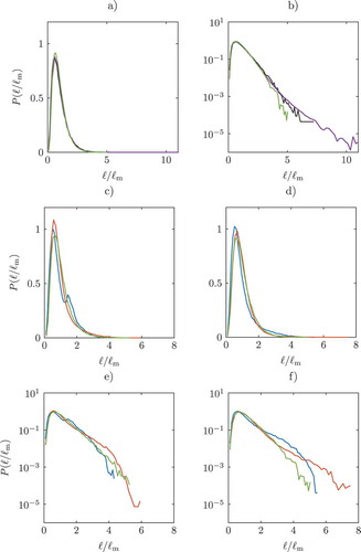
After a maximum, an exponential decrease of the PDF for longer DEs is observed, which is attributed to the cutting and connecting of the DEs by turbulent eddies (Wang and Peters, 2006). The exponential decrease of $P(\mathrm{\ell }/{\mathrm{\ell }}_{\mathrm{m}})$ is highlighted in Figure 5(b) by the linear logarithmic scale. The motion of turbulent eddies introduces new extremal points into the scalar fields altering the DE structure, effectively cutting a DE. If the probability of the occurrence of the turbulence-induced extremal point in the DE structure is independent of the location within the DE, $P(\mathrm{\ell }/{\mathrm{\ell }}_{\mathrm{m}})$ will decrease exponentially for large $\mathrm{\ell }/{\mathrm{\ell }}_{\mathrm{m}}$. The slope of the PDF in this representation indicates the cutting frequency, an inverse of an eddy turnover time (Wang, 2009). As previously observed (Wang, 2009; Wang and Peters, 2006), the Inert Isotropic case displays the exponential decrease. This is expected, as the isotropic nature of the case implies an eddy turnover time independent of the location and, consequently, a constant cutting frequency. However, the exponential decrease is also present in the PDFs of the Inert Temporally Evolving case and Inert Spatially Evolving case, with one and two statistically inhomogeneous directions, respectively. The slope of the exponential decrease of $P(\mathrm{\ell }/{\mathrm{\ell }}_{\mathrm{m}})$ is approximately the same for all Inert cases, resulting in a collapse of the PDFs in the range of scales dominated by random cutting and connecting range. Only in the tails of the PDFs, small differences can be observed. The Inert Isotropic case displays a range of normalized length scales comparable to that of the Spatial Evolving case. The greatest separation of scales is seen in the Inert Temporally Evolving case.

The PDFs for all spatially evolving cases for the upstream regions and downstream regions are shown in Figure 5(c and d). Again, the characteristic linear increase in the PDFs for the diffusive drift range is observed for the reacting and inert cases alike. The only difference in the characteristic shape of the PDFs is found in the upstream region of the spatially evolving cases. Here, the PDF of the Low Re Flame differs. While the PDFs of the High Re Flame and the Non-Reactive collapse, an additional local maximum in the Low Re Flame PDF is situated at $\mathrm{\ell }/{\mathrm{\ell }}_{\mathrm{m}}\approx 1.6$. This second maximum is a signature of a length scale induced at the nozzle that has not been sufficiently mixed out at this stream-wise location due to the limited level of turbulence in this case. In the PDFs at the downstream region in Figure 5(d), this initial length scale in the PDF was mixed out and the PDF took the expected form. Even though the Low Re and the Inert Spatial Evolving case share the same initial Reynolds number, the absence of the local maximum in the upstream region of the Spatial Evolving case is indicative of the fact that the passive scalar reaches an equilibrium in the length scale distribution further upstream of the nozzle, or in a temporal sense, faster than a reacting scalar, such as the temperature.

Figure 5(e and f) show the same PDFs in a linear logarithmic scale for the upstream and downstream regions, respectively. This representation highlights two distinctive characteristics. First, it shows the increasing scale separation due to increasing Reynolds number. While the PDFs agree well for the short DEs, the differences in the tails of the PDFs (long elements) are apparent. The High Re Flame displays the longest normalized DEs in both regions, while the Low Re Flame displays the smallest separation of length scales in the upstream position and the Inert Spatially Evolving case in the downstream regions. While the PDF of the Non-Reactive case shows hardly any difference in the two investigated region, the reacting cases show a significantly wider separation of scales in the downstream region. The non-reactive case displays an almost perfectly constant slope in both regions. The reactive cases show a constant slope for intermediate length comparable to the one observed in the Spatial Evolving case. For large ${\mathrm{\ell }}^{\ast }$, the discrepancy from the constant slope in the PDF can be explained by DEs that reach less turbulent regions where the cutting frequency is reduced due to heat release and higher viscosity and can, therefore, be attributed to low Reynolds number effects.

The invariance of the normalized DE length statistics toward changes in Reynolds numbers previously first observed by Wang and Peters (2006) holds for the premixed flames. However, the same characteristic shape of the PDFs of normalized length scales in the reacting scalars is surprising. Traditional methods of obtaining turbulent scales in reacting flows, such as spectra and structure functions, cannot be utilized to their fullest potential to generate equivocal results regarding the effect, or lack thereof, of combustion on turbulent scales due to the inherent high anisotropy and high intermittency of the investigated reacting flows.

Joint statistics of dissipation element parameter

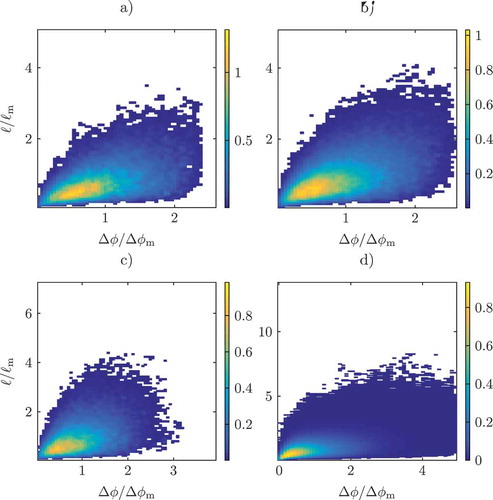
The second parameter characterizing DEs is the passive scalar difference $\mathrm{\Delta }\varphi$ in the Spatial Evolving cases and $\mathrm{\Delta }T$ in the reacting cases. Its analysis is performed by means of the jPDF of the normalized DE length ${\mathrm{\ell }}^{\ast }$ and the normalized scalar difference $\mathrm{\Delta }{\varphi }^{\ast }$, P($\mathrm{\Delta }{\varphi }^{\ast },{\mathrm{\ell }}^{\ast }$). The jPDFs are shown for the Spatial Evolving case for both the upstream and downstream regions in Figure 6(a and b). The maximum of the probability density is located in the bottom left corners for small values of ${\mathrm{\ell }}^{\ast }$and $\mathrm{\Delta }{\varphi }^{\ast }$. This region is characterized by the annihilation of short DEs due to the effect of the drift of extremal points. In the center of the jPDFs, the region dominated by the random cutting and reconnection of the DEs by turbulent eddies can be observed. The bottom right corner region characterized by short elements and large scalar differences corresponds to the so-called ‘cliff’ structures in scalar fields, cf. (Antonia and Sreenivasan, 1977; Holzer and Siggia, 1994). These DEs characterize regions of high scalar gradients followed by a gradual descent. The overall shapes of the jPDF in the two stream-wise regions agree well. In addition to the increasing separation in length scales from the upstream to the downstream region, already observed in the marginal statistics in Figure 4(c) and d), the range of the values of the normalized scalar difference increases as the flow is traversed in the stream-wise direction. The jPDF of the Inert Isotropic case in Figure 5(c) qualitatively shows the same shape as the one obtained from the Spatial Evolving case with a dominant maximum for small ${\mathrm{\ell }}^{\ast }$ and $\mathrm{\Delta }{\varphi }^{\ast }$ in the drift region. Only a slight difference for intermediate ${\mathrm{\ell }}^{\ast }$ and small $\mathrm{\Delta }{\varphi }^{\ast }$ can be observed, where the Inert Isotropic case shows a higher probability density. While the range of length scale values is similar, the Inert Isotropic case jPDF displays a larger range of values of $\mathrm{\Delta }{\varphi }^{\ast }$. Just as with the length scale separation in Figure 4(f), the Inert Temporally Evolving case shows the largest range of values for $\mathrm{\Delta }{\varphi }^{\ast }$. Otherwise the qualitative shape of the jPDF resembles that of the Spatial Evolving case. The jPDFs in Figure 4 closely resemble the jPDF obtained from the DE analysis of the mixture fraction field $Z$ of a planar temporally evolving non-premixed jet flame with a comparable Reynolds number to the Inert Temporally Evolving case in Gauding et al. (2017), which also displays a global maximum of the probability density in the diffusive drift region.

Figure 6. jPDFs of the normalized separation length $\mathrm{\ell }/{\mathrm{\ell }}_{\mathrm{m}}$ and the normalized scalar difference Δϕ/$\mathrm{\Delta }$ϕ_m. a): Spatial Evolving case upstream region. b): Spatial Evolving case downstream region. c): Inert Isotropic turbulence. d): Inert Temporally Evolving case.

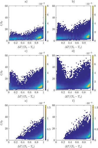
The normalization of DE parameters in the jPDF is also defined in a different fashion in order to compare DE scales with the characteristic flame thickness. In Figure 7, the normalization of $\mathrm{\ell }$ is performed with the laminar flame thickness δ_L (based on the temperature gradient) to achieve the originally proposed comparison of turbulent and flame scales ${\mathrm{\ell }}^{\prime }=\mathrm{\ell }/{\delta }_L$. The DE temperature difference is normalized with the temperature difference of the burned and unburned mixtures $\mathrm{\Delta }{T}^{\prime }=\mathrm{\Delta }T/(T_B-T_u)$. The maximum normalized value of $\mathrm{\Delta }{T}^{\prime }$= 1 corresponds to a DE whose gradient trajectories cross all the way from the unburned, through the premixed flame front to the fully burned. In Figure 7(a and b), the normalized jPDFs in the upstream region of the Low Re Flame and the High Re Flame are shown. For both cases, the maximum of the probability density is located in the right bottom corner for large $\mathrm{\Delta }{T}^{\prime }$ and small ${\mathrm{\ell }}^{\prime }$, placing large volumes of the flow in the ‘cliff’ structure regime. This ‘cliff’ structure is imposed by the ridged premixed flame structure on the temperature field, which cannot be fully mixed out by turbulent mixing and results in distinctly different shape of the jPDF as compared to the Spatial Evolving cases in Figure 6. Further, a local maximum is found in the diffusive drift region for small $\mathrm{\Delta }{T}^{\prime }$ and small ${\mathrm{\ell }}^{\prime }$ where approximately the global maximum is found for the Spatial Evolving cases. For scalar differences $\mathrm{\Delta }{T}^{\prime }$ < 0.5, the jPDFs resemble vaguely those of the non-reacting cases.

The small length scales remain constant while the integral scales increase with the Reynolds number, as intended in the configuration. The assumption of the regime of the “thin reaction zone” is reflected by the jPDFs as, while being on average larger than the flame thickness δ_L, the vast majority of the DEs are of a comparable length to the flame thickness. While not reaching all the way from the unburned to the burned, the flame structure remains largely intact with high probabilities of traversing large temperature differences before turbulence-induced extremal points interrupting the laminar flame structure. This is highly consistent with the conditions of the “thin reaction zones” where turbulent mixing interferes with the preheating zone dynamics while leaving the inner reaction zone unaffected, cf. Peters (2000). The jPDFs of the downstream region of the two reacting cases are shown in Figure 7(c and d). Again, a noticeable change in the stream-wise direction can be observed for both cases. While qualitatively resembling the jPDF of the upstream region, the jPDFs show a clear increase in length scales, as well as a further concentration of probability density in the global and local maximum.

In Figure 7(e and f), the jPDF in the downstream region of the Low Re and High Re Flame is conditioned on DEs which cross the flame front, omitting all non-reactive DEs from the statistics. The absence of the local maximum for small $\mathrm{\Delta }{T}^{\prime \prime }$ and small ${\mathrm{\ell }}^{\prime \prime }$ further indicates that this region corresponds to the core of the jet flow, as the similarity with the shape of the Spatial Evolving cases in Figure 5 already suggested. Both conditioned jPDFs look strikingly similar with regard to the range of values of the two DE parameters.

A similar conditioning of the DE statistics in reacting flows was applied to the jPDF of the mixture fraction field in a non-premixed jet in Gauding et al. (2017), where only DEs crossing the iso-surface of the stoichiometric mixture where retained in the statistics. While the scalar difference $\mathrm{\Delta }Z$ was higher in the reacting region of the non-premixed and ramp structures more probable, it was shown that this is caused by poor mixing in these regions. A drastic change in the shape of the jPDF with a clear imprint of the flame front, as displayed in Figure 7, was not observed.

Figure 7. jPDFs of the normalized separation length $\mathrm{\ell }/{\delta }_F$ and the normalized scalar difference $\mathrm{\Delta }T/(T_b-T_u)$. a): Low Re Flame upstream region. b): High Re Flame upstream region. c): Low Re Flame downstream region. d): High Re Flame downstream region. e): Low Re Flame downstream region conditioned on reacting DEs. f): High Re Flame downstream region conditioned on reacting DEs.

To achieve a quantitative comparison of the joint statistics of the normalized DE parameter statistics, the Kullbach-Leibler divergence $D_{\mathrm{K}\mathrm{L}}$ was computed. The Kullbach–Leibler divergence, applied to the joint statistics in this study, measures the logarithmic difference between the two jPDF of the normalized DE parameters $P_1(\mathrm{\Delta }{\varphi }^{\ast },{\mathrm{\ell }}^{\ast })$ and $P_2(\mathrm{\Delta }{\varphi }^{\ast },{\mathrm{\ell }}^{\ast })$ with reference to the latter and is defined as

$D_{\mathrm{K}\mathrm{L}}(P_1||P_2)=\int \underset{0}{\overset{\mathrm{\infty }}{\int }}{P}_1\left(\mathrm{\Delta }{\varphi }^{\ast },{\mathrm{\ell }}^{\ast }\right)log\frac{P_1\left(\mathrm{\Delta }{\varphi }^{\ast },{\mathrm{\ell }}^{\ast }\right)}{P_2\left(\mathrm{\Delta }{\varphi }^{\ast },{\mathrm{\ell }}^{\ast }\right)}\mathrm{d}\mathrm{\Delta }{\varphi }^{\ast }\mathrm{d}{\mathrm{\ell }}^{\ast }$

where two identical jPDF $P_1=P_2$ would yield $D_{\mathrm{K}\mathrm{L}}(P_1||P_2)=0$ The Kullbach–Leibler divergence between the Inert Isotropic case and the various other cases is shown in Figure 8(a).

Figure 8. a): Kullbach-Leibler divergence of the jPDFs of the normalized DE parameters of the various cases with reference to the jPDF obtained from the Inert Isotropic case. b): Kullbach-Leibler divergence of the marginal PDFs of the normalized DE length with reference to the Inert Isotropic case. The blue, red, and green diamonds correspond to the Low Re Flame, High Re Flame, and Spatial Evolving case, respectively. The solid symbols indicate the upstream region; the hollow and black dashed symbols indicate the downstream region. The Inert Temporally Evolving case is indicated by the solid purple triangle.

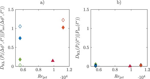
As expected from Figure 6, the Kullbach–Leibler divergence yields low values for the non-reacting cases indicating good agreement between the jPDFs and the jPDF of the Inert Isotropic case. For the Spatial Evolving case, the divergence decreases from the upstream to the downstream region, becoming almost identical to that of the isotropic turbulence. The reacting cases show $D_{\mathrm{K}\mathrm{L}}(P_{\mathrm{i}}||P_{\mathrm{i}\mathrm{s}\mathrm{o}})$ values at least an order of magnitude higher. Here, the trend with regard to the spatial change is reversed as the divergence increases from the upstream to the downstream region. As a point of reference, the Kullbach–Leibler divergences of the marginal PDF of the DE length is shown in Figure 8(b). $D_{\mathrm{K}\mathrm{L}}$ shows very low values for the marginal PDFs, regardless of the reactive or non-reactive nature of the case or stream-wise region. This further points to the DE scalar difference, which is almost exclusively affected by changes in configuration or the reactive nature of the scalar, while the normalized length scales remain unchanged.

The Kullbach–Leibler divergence of the jPDFs of the upstream and downstream regions of the spatially evolving cases yields values of $\text{0.1,left { lt,{D\_{{rm{KL}}}}({P\_{{rm{{it i},downstream}}}}}{rm{|}} right|,{P\_{{it i},{rm{upstream}}}}{rm{)}}, lt ,0.2}$, regardless of the reacting or non-reacting nature of the configuration, which indicates that the change in joint statistics is significantly more influenced by the reactive nature of the flames than the stream-wise region.

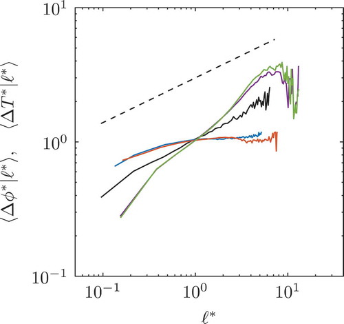
Finally, the normalized mean DE scalar difference conditioned on the normalized DE length $⟨\mathrm{\Delta }{\varphi }^{\ast }|{\mathrm{\ell }}^{\ast }⟩$ and $⟨\mathrm{\Delta }{T}^{\ast }|{\mathrm{\ell }}^{\ast }⟩$ is investigated in Figure 9. This conditional mean resembles a conditioned first-order moment of the respective scalar fields. For isotropic turbulence $⟨\mathrm{\Delta }{\varphi }^{\ast }|{\mathrm{\ell }}^{\ast }⟩$ was found to scale with Kolmogorov’s 1/3 power law, cf. Wang and Peters (2006, 2008)) and Schaefer et al. (2010). This scaling is reproduced with the Inert Isotropic case, which follows the scaling indicated by the dashed black line for large and intermediate lengths. The Inert Spatially Evolving case and the Inert Temporally Evolving case both show a clear scaling of $⟨\mathrm{\Delta }{\varphi }^{\ast }|{\mathrm{\ell }}^{\ast }⟩$ as well. However, this scaling is with an exponent of approximately 2/3, twice as high as the one obtained from the Inert Isotropic case. The perfect collapse of the two means in combination with the similarities of the jPDFs in Figure 6 seems to indicate that the differences between DE statistics of the spatial or temporal configuration is negligible. The difference in the scaling exponent can be attributed to the mean shear present in these flow configurations, which is absent in the Inert Isotropic case. The conditional means of the Low Re Flame and the High Re Flame collapse perfectly for the short and intermediate separation distances. Differences can only be observed for the large elements. However, both reacting cases display only a scaling for short elements, which ceases for DEs ${\mathrm{\ell }}^{\ast }>1$. For longer elements, the two DE parameters are uncorrelated.

Figure 9. Normalized mean DE scalar difference conditioned on the normalized DE length. The blue, red, and green lines indicate the Low Re Flame, High Re Flame, and Spatial Evolving case, respectively. The black line corresponds to the Inert Isotropic turbulence and the purple line to the Inert Temporally Evolving case. The dashed black line indicates Kolmogorov’s 1/3 power law scaling.

Conclusions

DE analysis was performed on the temperature fields of the DNS of two spatially evolving methane jet flames. Statistics of DE parameters were compared to those obtained from passive scalar fields of non-reacting flows including isotropic turbulence, a spatially evolving jet, and a temporally evolving jet to isolate individual effects of the reacting scalar on the DE statistics.

It was found that the DE length $\mathrm{\ell }$ was doubled in the temperature field compared to the passive scalar fields when normalized with the Kolmogorov micro-scale $\eta$. However, the invariance of the normalized statistics of $\mathrm{\ell }$ toward changes in Re observed in scalar fields in non-reacting flows was retained in the reacting cases.

Large differences in the statistics of the DE scalar difference $\mathrm{\Delta }T$ and $\mathrm{\Delta }\varphi$ between the reacting and the Spatial Evolving cases were observed, which could be attributed to the imprint of the premixed flame structure. The marginal and joint statistics showed a high consistency with the assumptions regarding the general setup of the reacting DNS and the regime of the thin reaction zones, with ${\mathrm{\ell }}_{\mathrm{m}}$ at least an order of magnitude higher than the flame thickness.

Acknowledgments

The authors acknowledge funding from of the European Research Council (ERC) under the European Union’s Horizon 2020 research and innovation program under grant agreement No 695747. In addition, the authors gratefully acknowledge the computing time provided by the JARA High Performance Computing Partition (JHPC09 and JHPC22) on the supercomputers JUQUEEN and JURECA at the Jülich Supercomputing Centre.

Additional information

Funding

This work was supported by the H2020 European Research Council [Advanced Grant (AdG), PE8, ERC-2015-AdG Milestone].

References

- Antonia, R.A., and Sreenivasan, K.R. 1977. Log-normality of temperature dissipation in a turbulent boundary layer. Phys. Fluids, 20, 1800–1804. doi:10.1063/1.861795
- Bisset, D.K., Julian, C.R., and Hunt, M.M.R. 2002. The turbulent/non-turbulent interface bounding a far wake. J. Fluid Mech., 451, 383–410. doi:10.1017/S0022112001006759
- Gampert, M., et al. 2011. Compressive and extensive strain along gradient trajectories in the turbulent kinetic energy field. New J. Phys., 13, 16.
- Gampert, M., Kleinheinz, K., Peters, N., and Pitsch, H. 2014. Experimental and numerical study of the scalar turbulent/non-turbulent interface in a Jet flow. Flow Turbul. Combust., 92, 429–449. doi:10.1007/s10494-013-9471-y
- Gampert, M., Schaefer, P., Goebbert, J.H., and Peters, N. 2013a. Decomposition of the field of the turbulent kinetic energy into regions of compressive and extensive strain. Physica Scripta, 155, 014002. doi:10.1088/0031-8949/2013/T155/014002
- Gampert, M., Schaefer, P., Narayanaswamy, V., and Peters, N. 2013b. Gradient trajectory analysis in a Jet flow for turbulent combustion modelling. J. Turbul., 14, 147–164. doi:10.1080/14685248.2012.747688
- Gampert, M., Schaefer, P., and Peters, N. 2013c. Experimental investigation of dissipation-element statistics in scalar fields in a jet flow. J. Fluid Mech., 724, 337–366. doi:10.1017/jfm.2013.171
- Gauding, M. 2014. Statistics and Scaling Laws of Turbulent Scalar Mixing at High Reynolds Numbers, RWTH Aachen University.
- Gauding, M., et al. 2017. Dissipation element analysis of a turbulent non-premixed jet flame. Phys. Fluids, 29.
- Holzer, M., and Siggia, E.D. 1994. Turbulent mixing of a passive scalar. Phys. Fluids, 6, 1820–1837. doi:10.1063/1.868243
- Hunger, F., Gauding, M., and Hasse, C. 2016. On the impact of the turbulent/non-turbulent interface on differential diffusion in a turbulent jet flow. J. Fluid Mech., 802.
- Luca, S., Al-Khateeb, A.N., Attili, A., and Bisetti, F. 2018. Comprehensive validation of skeletal mechanism for turbulent premixed methane–air flame simulations. J. Prop. Power, 34.1, 153–160. doi:10.2514/1.B36528
- Luca, S., Attili, A., et al. 2019. On the statistics of flame stretch in turbulent premixed jet flames in the thin reaction zone regime at varying Reynolds number. Proc. Combust. Inst, 37, 2451–2459.
- Peters, N. 2000. Turbulent Combustion, Cambridge University Press.
- Peters, N., Kerschgens, B., and Paczko, G. 2013. Super-Knock prediction using a refined theory of turbulence. SAE Int. J. Engines, 6, 953–967. doi:10.4271/2013-01-1109
- Peters, N., and Wang, L. 2006. Dissipation element analysis of scalar fields in turbulence. C. R. Mechanique, 334, 493–506. doi:10.1016/j.crme.2006.07.006
- Schaefer, L., et al. 2011. Investigation of dissipation elements in a fully developed turbulent channel flow by tomographic-particle image velocimetry. Phys. Fluids, 23. doi:10.1063/1.3556742
- Schaefer, P., Gampert, M., Goebbert, J., Wang, L., Peters, N. 2010. Testing of Model Equations for the Mean Dissipation using Kolmogorov Flows, Flow, Turbulence and Combustion, 85 (2): 225–243. doi:10.1007/s10494-010-9273-4
- Scholtissek, A., Dietzsch, F., Gauding, M., and Hasse, C. 2017. No In-situ tracking of mixture fraction gradient trajectories and unsteady flamelet analysis in turbulent non-premixed combustion. Comb. Flame, 243–258. doi:10.1016/j.combustflame.2016.07.011
- Wang, L. 2009. Structure function of two-point velocity difference along scalar gradient trajectories in fluid turbulence. Phys. Rev. E, 79.
- Wang, L., and Peters, N. 2006. The length scale distribution function of the distance between extremal points in passive scalar turbulence. J. Fluid Mech., 554, 457–475. doi:10.1017/S0022112006009128
- Wang, L., and Peters, N. 2008. The Length scale distribution functions and conditional means for various fields in turbulence. J. Fluid Mech., 608, 113–138. doi:10.1017/S0022112008002139