Effects of spatial distribution of CO2 dilution on localised forced ignition of stoichiometric biogas-air mixtures

ABSTRACT

The localized forced ignition and subsequent flame propagation have been analyzed for stoichiometric biogas-air mixtures ($\mathrm{C}{\mathrm{H}}_4/\mathrm{C}{\mathrm{O}}_2/\mathrm{a}\mathrm{i}\mathrm{r}$ blend) with different spatial distributions (uniform, Gaussian and bimodal) and mean levels of $\mathrm{C}{\mathrm{O}}_2$ dilution (i.e. mole fraction of $\mathrm{C}{\mathrm{O}}_2$) for different flow conditions (e.g. quiescent laminar condition and different turbulence intensities) using three-dimensional Direct Numerical Simulations. A two-step chemical mechanism with sufficient accuracy is used to capture the effects of $\mathrm{C}{\mathrm{O}}_2$ dilution on the laminar burning velocity of the $\mathrm{b}\mathrm{i}\mathrm{o}\mathrm{g}\mathrm{a}\mathrm{s}-\mathrm{a}\mathrm{i}\mathrm{r}\mathrm{m}\mathrm{i}\mathrm{x}\mathrm{t}\mathrm{u}\mathrm{r}\mathrm{e}$. A parametric analysis in terms of the mean, standard deviation and integral length scale of the initial Gaussian and bimodal distributions of spatial $\mathrm{C}{\mathrm{O}}_2$ dilution in the unburned gas has been conducted. Qualitatively similar behavior has been observed for all three initial spatial distributions of $\mathrm{C}{\mathrm{O}}_2$. A departure from uniform conditions was found to increase the range of reaction rate magnitudes of $\mathrm{C}{\mathrm{H}}_4$, which impacts the burned gas volume and, in turn, increases the variability of the outcomes of the ignition event (successful thermal runaway and subsequent self-sustained propagation or misfire). Turbulence intensity and the mean level of dilution were found to have significant impacts on the outcome of the localized forced ignition, and an increase of either quantity acts to reduce the burned gas volume irrespective of mixture composition due to the enhancement of heat transfer from the hot gas kernel, and the heat sink effects of $\mathrm{C}{\mathrm{O}}_2$, respectively. An increase of the integral length scale $l_{\psi }$ for the spatial distribution of $\mathrm{C}{\mathrm{O}}_2$ dilution increased the probability of a successful outcome of the ignition event. A uniform initial spatial distribution was found to be optimal, and in the case of a departure from non-uniform conditions, larger variability in the outcome are obtained for a Gaussian initial distribution of $\mathrm{C}{\mathrm{O}}_2$ dilution than a bimodal one. The variance of the $\mathrm{C}{\mathrm{O}}_2$ dilution distribution has been found to have a negligible impact on the outcomes observed, as it was dominated by the effects arising from turbulence intensity, nature of initial $\mathrm{C}{\mathrm{O}}_2$ distribution and integral length scale of $\mathrm{C}{\mathrm{O}}_2$ dilution.

KEYWORDS:

• Localized forced ignition
• biogas-air mixture
• co₂ dilution
• turbulence intensity
• direct numerical simulations

INTRODUCTION

Interest in alternative fuel solutions has increased over the years, and the transportation industry and governments are making a concerted effort to move to renewable and eco-friendly solutions to meet ever more stringent emissions and pollution standards (Koonaphapdeelert, Aggarangsi, Moran 2020; Korberg, Skov, Mathiesen 2020; Mustafi and Agarwal 2020; Patterson et al. 2011; Rafiee et al. 2021). Despite electric vehicles being heralded as the future of the industry, the use of the internal combustion engine is expected to play a dominant role for the upcoming decades due to existing investment in such technologies along with its widespread use. Additionally, in remote locations and developing countries, the infrastructure required to be able to efficiently utilize electric cars is still lacking. In many of these places, the cost of conventional fossil fuels is high, and thus there is a demand for solutions that are cost-effective, renewable, efficient and functional under a wide range of operating conditions. One solution which has been gaining traction in recent years in Singapore (Koonaphapdeelert, Aggarangsi, Moran 2020; Mustafi and Agarwal 2020), Middle East (IRENA 2018), Eastern Europe (Papacz 2011) and Nordic (Persson 2007) countries, is the alteration of internal combustion engines operating on fossil fuels to operate them using Biogas-air mixtures for personal and light commercial vehicles (Barik and Murugan 2014; Crookes 2006; Jatana et al. 2014; Shah et al. 2017). The modifications required for such an alteration are straightforward, cheap, and allow the vehicle not only to run using solely fossil fuels as originally designed, but also to operate using a mixture consisting primarily of biogas mixed with the existing fuel (EU and Bluesky 2018; Surataa et al. 2014). One of the problems with the use of biogas in internal combustion engines for personal vehicles is that the efficiency and stability of the biogas-fueled engine are worse than that obtained for the fuel with which the engine was originally designed to operate. This is further amplified by inconsistencies and impurities in the fuel blend (Barik and Murugan 2014; EU and Bluesky 2018; Jatana et al. 2014; Ryckebosch, Drouillon, Vervaeren 2011; Shah et al. 2017; Surataa et al. 2014).

Biogas is primarily composed of $\mathrm{C}{\mathrm{H}}_4$ and $\mathrm{C}{\mathrm{O}}_2$, but the production of industrial quantities of biogas with a fixed composition is hard due to its biological origins (Rasi, Veijanen, Rintala 2007; Ryckebosch, Drouillon, Vervaeren 2011). Depending on the production method used, biogas can be a carbon-neutral fuel and due to existing natural gas infrastructure, it can easily be stored and transported whilst also being used in conjunction with natural gas for power generation and transportation. Additional advantages of biogas are that it can be produced locally whilst offering an eco-friendly solution to disposing of sewage and agricultural waste. For example, sewage can be used to produce the biogas to power the waste collection trucks (https://www.csmonitor.com/Environment/Living-Green/2010/0107/California-garbage-trucks-fueled-by-garbage). Due to its organic nature, its storage is significantly less risky than that of fossil fuels, making it an attractive energy source for smaller countries looking to become energy independent and move to renewable energy production. In-depth reviews (Koonaphapdeelert, Aggarangsi, Moran 2020; Korberg, Skov, Mathiesen 2020; Mustafi and Agarwal 2020; Patterson et al. 2011; Rafiee et al. 2021) of biogas utilization ranging from instructional to a high technical level have been published to aid the efficiency of biogas utilization. These reviews indicate that biogas utilization and upgrading is still a developing field, with a strong demand on both micro (personal) and macro (governmental and institutional) levels, for the numerous reasons mentioned above. Another advantage of using biogas blended with fossil fuels is the significant reduction of emissions and soot formations, whilst engine performance is not severely impacted (Crookes 2006; EU and Bluesky 2018; Jatana et al. 2014; Shah et al. 2017; Surataa et al. 2014). However, these findings have been obtained under laboratory conditions where the fuel composition and mixing are fully controlled. Of particular interest is the preprocessing of the biogas to reduce sulfur and other trace species impurities (Rasi, Veijanen, Rintala 2007; Ryckebosch, Drouillon, Vervaeren 2011; Surataa et al. 2014), along with the perfect premixing of the combustible mixture, which is achieved under controlled laboratory conditions. The impurities present in the biogas mixture fall outside of the scope of this study, however the perfect mixing achieved under laboratory conditions is difficult to achieve in practice, and thus the ignition and subsequent combustion of biogas-air mixtures can take place under inhomogeneous conditions in real-life applications. Thus, the mixture can have significant variations in the composition encountered at different locations in the combustion chamber, which can lead to a reduction of performance or even misfires. Hence, the forced ignition of inhomogeneous biogas-air mixtures has significant applications in direct-injection engines in the automotive industry, and energy production methods involving biogas.

Previous studies (Forsich et al. 2004; Lafay et al. 2007; Lieuwen et al. 2008; Mulla et al. 2016; Rasi, Veijanen, Rintala 2007; Ryckebosch, Drouillon, Vervaeren 2011; Vasavan, De Goey, van Oijen 2018) have shown that variations in $\mathrm{C}{\mathrm{O}}_2$ content can influence the localized forced ignition (e.g. spark and laser ignition) performance, leading to adverse effects on the subsequent flame propagation. Existing studies (Galmiche et al. 2011; Larsson, Berg, Bonaldo 2013), which investigated forced ignition of biogas-air mixtures, have focussed on perfectly premixed biogas-air mixtures with a fixed level of $\mathrm{C}{\mathrm{O}}_2$ content. This, in turn, leads to a uniform spatial distribution of the $\mathrm{C}{\mathrm{O}}_2$ content leading to homogeneous mixtures being encountered at all points of the combustion chamber. However, the effects of the non-uniform composition of biogas encountered locally have not been analyzed to date. Galmiche et al. (2011) reported that $\mathrm{C}{\mathrm{O}}_2$ acts as a heat sink, and an increase in the amount of $\mathrm{C}{\mathrm{O}}_2$ dilution leads to an increase in the energy required for a successful ignition, and that successful ignition was possible for mixtures with up to 40% (by volume) $\mathrm{C}{\mathrm{O}}_2$ dilution. A large modification of the reaction zone (Lafay et al. 2007) and a hindrance to flame kernel formation were found by both Mordaunt and Pierce (2014) and Lafay et al. (2007) for biogas/air mixtures in a gas turbine configuration. The lower burning velocity of biogas-air mixtures in comparison to methane-air mixtures leads to a slower combustion process (Galmiche et al. 2011; Larsson, Berg, Bonaldo 2013). The presence of $\mathrm{C}{\mathrm{O}}_2$ in the fuel can potentially lead to flame extinction (lean blow-out) (Mordaunt and Pierce 2014). Industrial demand to ignite gas turbines using the fuel available on offshore plants led Larsson, Berg, and Bonaldo (2013) to experimentally investigate the minimum ignition energy (MIE) required for successful ignition across hydrocarbon fuels mixed with inert gases. Nitrogen and carbon dioxide were separately used as the diluents, and mixed with methane and propane mixtures individually, in order to find the maximum level of diluent which could be present in each gas composition, whilst also being able to be successfully ignited. The above experimental studies indicate that an increase in the amount of $\mathrm{C}{\mathrm{O}}_2$ is detrimental toward successful thermal runaway and subsequent self-sustained combustion, indirectly highlighting the importance of the fuel composition in terms of diluent that the flame kernel encounters.

Ever more detailed Direct Numerical Simulations (DNS) of localized forced ignition events in gaseous mixtures have become feasible due to the increase in computational power over the last decade. These advancements have provided improved physical insights into the ignition process and subsequent flame propagation. Pera, Chevillard, and Reveillon (2013) demonstrated that the mixture inhomogeneity induced by residual burnt gas has significant influence on early flame propagation and cyclic variability in the case of forced ignition using DNS. Further numerical investigations were carried out by Patel and Chakraborty (2014; 2015, 2016a-c) to analyze the effects of turbulence intensity on forced ignition of stratified mixtures. It was found that an increase of turbulence intensity with a fixed length scale has a detrimental effect on successful ignition. Patel and Chakraborty (2016c) also focussed on the effects of initial mixture distribution (i.e. variance and length scale of equivalence ratio), where the equivalence ratio was initialized using both Gaussian and bimodal distributions, to investigate the effects of different initial distributions on the localized forced ignition of globally stoichiometric stratified mixtures. An increase in the burning rate was observed when the initial equivalence ratio distribution was Gaussian as opposed to bimodal. However, for the Gaussian initial distribution a higher possibility of flame extinction was observed for large values of turbulence intensity, in comparison to the bimodal distribution. Three-dimensional simple chemistry DNS was also used by Patel and Chakraborty (2016a-c) to investigate the influence of turbulence intensity, fuel Lewis number and mixture fraction gradient on ignition success and subsequent flame propagation characteristics in turbulent stratified mixtures. In a recent DNS analysis (Turquand d’Auzay et al. 2019a) by the present authors, the variations of turbulence intensity and dilution levels on the localized forced ignition of turbulent mixing layers of $\mathrm{C}{\mathrm{H}}_4-\mathrm{C}{\mathrm{O}}_2-\mathrm{a}\mathrm{i}\mathrm{r}$ for different extents of $\mathrm{C}{\mathrm{O}}_2$ dilution with $\mathrm{C}{\mathrm{H}}_4-$air mixtures have been investigated, which demonstrated that an increase in $\mathrm{C}{\mathrm{O}}_2$ dilution leads to reductions of burning rate and the probability of obtaining self-sustained combustion once the ignitor is switched off. Interested readers are referred to Mastorakos (2009) for a comprehensive review of different aspects of forced ignition for both homogeneous and inhomogeneous mixtures.

Existing computational investigations (Chakraborty, Cant, Mastorakos 2007; Chakraborty and Mastorakos 2008; Patel and Chakraborty 2014, 2015, 2016a-c; Turquand d’Auzay et al. 2019b) focused primarily on single fuels such as methane or hydrogen but not compound fuels such as biogas. To be more specific, the effects arising from the spatial distribution of the diluent of choice (i.e $\mathrm{C}{\mathrm{O}}_2$ for biogas) on the localized forced ignition and subsequent flame propagation have not yet been investigated either experimentally or computationally to the best of the authors’ knowledge. Thus, a systematic parametric study has been carried out across a range of different turbulence intensities, concentrating on the effects of the nature of the spatial distribution (uniform, Gaussian and bimodal) of $\mathrm{C}{\mathrm{O}}_2$ dilution and their characteristics (i.e. mean, variance and integral length scale of $\mathrm{C}{\mathrm{O}}_2$ dilution) in the case of localized forced ignition of stoichiometric biogas-air mixtures (assumed to be $\mathrm{C}{\mathrm{H}}_4$+$\mathrm{C}{\mathrm{O}}_2$-air mixtures). Thus, the objectives of this paper are:

(a) to demonstrate the effects of different spatial distributions (uniform, Gaussian and bimodal) of $\mathrm{C}{\mathrm{O}}_2$ dilution on the localized forced ignition of stoichiometric biogas-air mixtures.

(b) to provide physical explanations for the observed influence of different initial $\mathrm{C}{\mathrm{O}}_2$ distributions on the burning rate characteristics of stoichiometric biogas-air mixtures.

The mathematical background and numerical framework pertaining to the current analysis are presented in the next two sections. This is followed by the presentation of results along with their discussion. The main findings are summarized, and conclusions are drawn in the final section of this paper.

MATHEMATICAL BACKGROUND

The following global equation represents the stoichiometric combustion of biogas represented by a $\mathrm{C}{\mathrm{H}}_4+\mathrm{C}{\mathrm{O}}_2$ mixture:

(1) $\mathrm{C}{\mathrm{H}}_4+2\left({\mathrm{O}}_2+3.76{\mathrm{N}}_2\right)+a\cdot \mathrm{D}\mathrm{i}\mathrm{l}\mathrm{u}\mathrm{e}\mathrm{n}\mathrm{t}\to \mathrm{C}{\mathrm{O}}_2+2{\mathrm{H}}_2\mathrm{O}+7.52{\mathrm{N}}_2+a\cdot \mathrm{D}\mathrm{i}\mathrm{l}\mathrm{u}\mathrm{e}\mathrm{n}\mathrm{t}$(1)

and the level of dilution with $\mathrm{C}{\mathrm{O}}_2$ present in the biogas-air mixture is quantified in terms of the unburnt mixture according to the definition presented by Galmiche et al. (2011):

(2) ${\psi }^u=\frac{a}{a+1+2+7.52}=\frac{a}{a+10.52}$(2)

where ${\psi }^u$ represents the dilution percentage which is the molar fraction of the diluent ($\mathrm{C}{\mathrm{O}}_2$) in the unburned gases and $a$ represents the stoichiometric coefficient, as shown in Eq. 1(1) $\mathrm{C}{\mathrm{H}}_4+2\left({\mathrm{O}}_2+3.76{\mathrm{N}}_2\right)+a\cdot \mathrm{D}\mathrm{i}\mathrm{l}\mathrm{u}\mathrm{e}\mathrm{n}\mathrm{t}\to \mathrm{C}{\mathrm{O}}_2+2{\mathrm{H}}_2\mathrm{O}+7.52{\mathrm{N}}_2+a\cdot \mathrm{D}\mathrm{i}\mathrm{l}\mathrm{u}\mathrm{e}\mathrm{n}\mathrm{t}$(1) . The level of dilution present can also be defined based on the dilution in the $\mathrm{C}{\mathrm{H}}_4+\mathrm{C}{\mathrm{O}}_2$ mixture as:

(3) ${\psi }^f=\frac{a}{a+1}=\frac{Y_{C{O}_2}/M{W}_{C{O}_2}}{(Y_{C{O}_2}/M{W}_{C{O}_2})+(Y_{C{H}_4}/M{W}_{C{H}_4})}$(3)

where $Y_{C{O}_2}$ and $Y_{C{H}_4}$ are mass fractions of $\mathrm{C}{\mathrm{O}}_2$ and $\mathrm{C}{\mathrm{H}}_4$ respectively and $M{W}_{C{O}_2}$ and $M{W}_{C{H}_4}$ are the molecular weights of $\mathrm{C}{\mathrm{O}}_2$ and $\mathrm{C}{\mathrm{H}}_4$ respectively. Thus, ${\psi }^f$ represents the molar fraction of the diluent present in the $\mathrm{C}{\mathrm{H}}_4+\mathrm{C}{\mathrm{O}}_2$ mixture. To account for the effects of dilution with $\mathrm{C}{\mathrm{O}}_2$ and to also allow for the study to be computationally feasible (in terms of cost), a two-step chemical mechanism (Bibrzycki and Poinsot 2010; Westbrook and Dryer 1981) has been used for the present analysis. It should be noted that the cases considered for the present analysis constute a large parametric analysis involving more than 350 different three-dimensional simulations. It becomes impractical to carry out such a parametric analysis based on detailed chemistry because the computational cost becomes exorbitant (Chen et al., 2009). Typically, a detailed chemistry simulation for a skeletal mechanism of methane-air combustion involving 16 species and 25 reactions (Smooke and Giovangigli 1991) is roughly 20 times more expensive than one of the simulations conducted for this analysis. Thus, it is impossible to carry out the analysis conducted here using even a skeletal chemical mechanism. Therefore, the chemical representation in this analysis is simplified here by a two-step mechanism which involves incomplete oxidation of $\mathrm{C}{\mathrm{H}}_4$ into $\mathrm{C}\mathrm{O}$, and an equilibrium reaction between oxidation of $\mathrm{C}\mathrm{O}$ to $\mathrm{C}{\mathrm{O}}_2$ and dissociation of $\mathrm{C}{\mathrm{O}}_2$ into $\mathrm{C}\mathrm{O}$. It is worth noting that pioneering analytical studies (Champion et al. 1986; Espí and Liñán 2001, 2002; He 2000; Sibulkin and Siskind 1987) on ignition have been conducted for single-step irreversible Arrhenius type chemistry.

Several assumptions are made in the present analysis for the purpose of simplicity, and to also allow for the simulations to be computationally feasible. The Lewis number of all species is taken to be equal to unity, and all species in the gaseous phase are taken to be ideal gases, and thus the ideal gas law is used for compressible flow DNS. The species included are CH₄, CO, CO₂, N₂, H₂O and O₂ whose Lewis numbers are bounded by $0.8\le Le\le 1.39$ and thus, the unity Lewis number assumption does not significantly introduce any inaccuracy in a qualitative sense. This was also confirmed in previous analytical (He 2000; Sibulkin and Siskind 1987) and DNS (Chakraborty, Hesse, Mastorakos 2010; Patel and Chakraborty 2016a) studies. The ratio of specific heats ($\gamma =C_P^g/C_v^g=1.4$, where $C_p^g$ and $C_v^g$ are the gaseous specific heats at constant pressure and volume, respectively) and Prandtl number ($Pr=\mu C_p^g/\lambda =0.7$, where $\mu$ is the dynamic viscosity and $\lambda$ is the thermal conductivity of the gaseous phase) take standard values, respectively. Fick’s law of diffusion is used to account for the species diffusion velocity. The unburned gas mixture is preheated to $T_0=590K$ to reduce the error made by using the assumption of equal specific heat for all species as the heat capacities of $\mathrm{C}{\mathrm{O}}_2$ and ${\mathrm{N}}_2$ become equal to each other at $600K$. For lower temperatures (e.g. $300K$), the difference in heat capacity is as high as 40%. For higher temperatures, ($>600K$) the difference of the heat capacity between the two species is at most 6%. Furthermore, as the gaseous mixture is predominantly composed of ${\mathrm{N}}_2$ for small values of ${\psi }^f$, the heat capacity of the gaseous mixture would be very close to that of ${\mathrm{N}}_2$. This, in turn, means that the errors introduced by the assumption of equal specific heat are small. In this analysis, the specific heat at constant pressure $C_p$, dynamic viscosity $\mu$, thermal conductivity $\lambda$ and the density-weighted mass diffusivity $\rho D$ are considered to be constant for the sake of simplicity following previous analyses (Chakraborty and Mastorakos 2006; Hesse, Chakraborty, Mastorakos 2009; Wandel, Chakraborty, Mastorakos 2009; Hesse, Malkeson, Chakraborty 2012; Papapostolou et al. 2019, 2021; Turquand d’Auzay et al. 2019a; Turquand d’Auzay, Papapostolou, Chakraborty 2021), which ensures that the Lewis number does not change within the flame. The constant thermophysical properties do not alter the mixing statistics in the unburned gas. For simulations with temperature-dependent thermophysical properties, the increased viscosity can lead to faster decay of turbulence which limits the extent of flame-turbulence interaction that can be analyzed using DNS because of moderate values of turbulent Reynolds number. Moreover, the mass diffusivity increases within the flame more rapidly in the simulations with temperature-dependent thermophysical properties than that obtained in the case of constant thermophysical properties. This implies that the mixture inhomogeneity decays faster in the case of temperature-dependent thermophysical properties than that in the case of constant thermophysical properties, and this limits the extent to which mixture inhomogeneity effects can be studied using DNS for moderate values of turbulent Reynolds number. Poinsot, Echekki, and Mungal (1992) observed that the stretch rate dependence of flame displacement speed for constant thermophysical properties is qualitatively similar to that obtained for temperature-dependent thermophysical properties for simple chemistry, but quantitative differences do exist. It was also demonstrated by Aspden (2017) that the constant viscosity assumption does not affect the qualitative nature of the flame morphology and vorticity distribution across the statistically planar turbulent premixed flames. However, the analyses by Poinsot et al. (2019) and Aspden (2017) are not done in the context of localized forced ignition of biogas-air mixtures, and therefore further analyses on forced ignition of biogas-air mixtures in the presence of temperature-dependent thermophysical properties will be needed to ascertain the extent of qualitative similarities between variable and constant thermophysical properties. It is worth noting that the the Chapman-Rubesin variable transport model can potentially offer a realistic dependence of transport properties on temperature without increasing the computational cost but its application to DNS of localized forced ignition is beyond the scope of current investigation. However, this aspect deserves further investigation in the future.

The two-step chemical mechanism along with the transport model selected for this analysis has been validated against other chemical mechanisms (GRI-Mech 3.0 (Smith et al. 1995) and 2s_CM2 (Bibrzycki and Poinsot 2010; Selle et al. 2004)) and experimental results (Galmiche et al. 2011) for both $\mathrm{C}{\mathrm{H}}_4$ and $\mathrm{C}{\mathrm{H}}_4+\mathrm{C}{\mathrm{O}}_2$ mixtures under all the above simplifying assumptions. For large values of ${\psi }^u$ (e.g. ${\psi }^u>0.10$), the two-step chemical mechanism overestimates the laminar burning velocity, and thus the maximum level of mean dilution investigated in the present study is ${\psi }^u=0.10$, for which flame speed predictions are sufficiently accurate (Turquand d’Auzay et al. 2019a). For further details regarding the performance and validation of the mechanism, interested readers are directed to recent work by Turquand d’Auzay et al. (2019a).

It is important to note that the chemical mechanism used in this analysis has been benchmarked for flame propagation and simplifications for the transport quantities are made in the interest of a detailed parametric analysis. In the case of forced ignition, the temperature attained during the external energy deposition duration is high enough to result in a very small value of ignition delay time. Therefore, inaccuracies in the ignition delay prediction do not significantly affect the results presented in this paper because the subsequent flame kernel development is principally determined by the flame propagation. Moreover, the seminal DNS analysis by Mastorakos, Baritaud, and Poinsot (1997) with single-step Arrhenius type chemistry revealed that the reaction rate magnitude of fuel and scalar dissipation rate are negatively correlated in the case of autoignition, which was found to be qualitatively similar in subsequent detailed chemistry DNS studies (Im, Chen, Law 1998). Recently, it has been demonstrated by the authors (Papapostolou, Turquand d’Auzay, Chakraborty 2020) that the MIE variation with turbulence intensity for the stoichiometric homogeneous mixed biogas-air mixture using this chemical mechanism provides excellent qualitative and quantitative agreements between DNS and experimental (Cardin et al. 2013a, 2013b) results. Moreover, the flame structure resulting from localized forced ignition of turbulent gaseous mixing layer and droplet-laden mixtures using single step Arrhenius type chemistry (Chakraborty and Mastorakos 2006, 2008; Papapostolou et al. 2019) are qualitatively similar to those obtained from detailed chemistry simulations (Ray et al., 2001; Neophytou, Mastorakos, Cant 2010). Turquand d’Auzay, Papapostolou, and Chakraborty (2021) demonstrated that the edge flame propagation statistics for forced ignition of turbulent mixing layers for the chemical and transport models used in this paper are qualitatively similar to the results obtained from detailed chemistry DNS studies (Echekki and Chen 1998; Im and Chen 1999, 2001). Furthermore, it has been found that the statistical behaviors of the edge flame displacement speed including its strain rate, curvature, and scalar gradient dependences from simple single-step chemistry DNS data (Chakraborty, Hesse, Mastorakos 2010; Chakraborty and Mastorakos 2006; Hesse, Chakraborty, Mastorakos 2009; Hesse, Malkeson, Chakraborty 2012; Karami et al. 2015, 2016) have been found to be qualitatively consistent with detailed chemistry DNS (Echekki and Chen 1998; Im and Chen 1999, 2001) and experimental (Chung 2007; Heeger et al. 2009; Ko and Chung 1999) findings. In addition, the current analysis adopts a chemical mechanism which is more detailed in comparison to several previous analyses (Chakraborty and Mastorakos 2006; Hesse, Chakraborty, Mastorakos 2009; Hesse, Malkeson, Chakraborty 2012; Karami et al. 2015, 2016).

Due to the large computational cost associated with DNS and the large parameter space covered in this work, a canonical configuration which considers solely the volume surrounding the energy deposition location (i.e. the ignition site) has been used. This approach was followed in several previous studies on ignition (Bansal and Im 2011; Hawkes et al. 2006; Pera, Chevillard, Reveillon 2013; Sankaran et al. 2005; Yu and Bai 2010) and the same approach was followed in this study. Due to the canonical nature of the simulation domain in DNS, the results obtained from these analyses are mostly qualitative in nature and therefore the simplifications made in this analysis do not significantly affect the conclusions made from this analysis.

The mixture fraction $\xi$ is used to describe the mixture composition and is defined using Bilger’s definition (Bilger 1980) as

(4) $\xi =\frac{\beta -{\beta }_o}{{\beta }_f-{\beta }_o}$(4)

where ${\beta }_o$ and ${\beta }_f$ are the values of $\beta$ in the oxidizer and fuel streams respectively, with $\beta =2Y_C/W_C+Y_H/2W_H-Y_O/W_O$, and $Y_k$ and $W_k$ denoting the atomic mass fractions and molecular weights. The stoichiometric mixture fraction value is defined as (Bilger 1980)

(5) ${\xi }_{st}=-\frac{{\beta }_o}{{\beta }_f-{\beta }_o}$(5)

A reaction progress variable $c$ that increases monotonically from zero in the unburned mixture to unity in the products is used to measure the extent of the completion of chemical reactions, and in the present study is defined based on the fuel mass fraction as (Chakraborty, Cant, Mastorakos 2007; Chakraborty, Hesse, Mastorakos 2010; Chakraborty and Mastorakos 2008; Turquand d’Auzay et al. 2019a)

(6) $c=\frac{\xi Y_{F_{\mathrm{\infty }}}\left({\psi }^f\right)-Y_F}{\xi Y_{F_{\mathrm{\infty }}}\left({\psi }^f\right)-max\left(0,\frac{\xi -{\xi }_{st}}{1-{\xi }_{st}}\right){Y_F}_{\mathrm{\infty }}\left({\psi }^f\right)}$(6)

where $Y_{F_{\mathrm{\infty }}}$ is the mass fraction of fuel ($\mathrm{C}{\mathrm{H}}_4$) in the pure fuel stream, whilst ${\psi }^f$ within brackets indicates values that correspond to that level of $\mathrm{C}{\mathrm{O}}_2$ dilution. The reaction progress variable can also be defined in terms of oxidizer mass fraction, however in the present study the choice of the reaction progress variable definition does not affect the qualitative nature of the findings.

Following previous studies (Chakraborty, Cant, Mastorakos 2007; Chakraborty and Mastorakos 2008; Chakraborty, Hesse, Mastorakos 2010; Turquand d’Auzay et al. 2019a,b; Wandel, Chakraborty, Mastorakos 2009) on localized forced ignition, only the thermal effects have been accounted for and the details of the spark formation (momentum modification contribution, plasma and shock wave formation) are not considered in this analysis for the purpose of simplicity and computational economy. An additional source term, $(q^{\prime \prime \prime }=A_{sp}exp\left(-r^2/2R_{sp}^2\right)$ with $r$ being the distance from the ignitor center, which is taken to be the geometric center of the domain, and $R_{sp}$ represents the characteristic width of energy deposition (Espí and Liñán 2001, 2002)) is added to the energy conservation equation to account for the effects of the localized forced ignition (Chakraborty, Cant, Mastorakos 2007; Chakraborty and Mastorakos 2008; Chakraborty, Hesse, Mastorakos 2010; Turquand d’Auzay et al. 2019a,b; Wandel, Chakraborty, Mastorakos 2009). The constant $A_{sp}$ in the source term $q{ }^{\mathrm{\prime }\mathrm{\prime }\mathrm{\prime }}$ is determined by a volume integration which leads to the total ignition power $\dot{Q}$ in the following manner (Chakraborty, Cant, Mastorakos 2007; Chakraborty and Mastorakos 2008; Chakraborty, Hesse, Mastorakos 2010; Turquand d’Auzay et al. 2019a,b; Wandel, Chakraborty, Mastorakos 2009)

(7) $\dot{Q}=\underset{V}{\int }q{ }^{\mathrm{\prime }\mathrm{\prime }\mathrm{\prime }}dV=a_{sp}{\rho }_0{C}_p\tau T_0\left(\frac{4}{3}\pi \delta {{ }_z^0}^3\right)\left[\frac{H\left(t\right)-H\left(t-t_{sp}\right)}{t_{sp}}\right]$(7)

where $a_{sp}$ is a parameter determining the total energy deposited by the ignitor, $\tau =\left(T_{ad}^0-T_0\right)/T_0$ is the heat release parameter (where $T_{ad}^0$ and $T_0$ are the adiabatic flame temperature of the undiluted stoichiometric $\mathrm{C}{\mathrm{H}}_4$-air mixture and unburned gas temperature respectively), ${\delta }_z^0$ is the Zel’dovich flame thickness of the undiluted stoichiometric methane-air mixture (${\delta }_z^0=D_0/s_l^0$, where $D_0$ is the unburned mass diffusivity of the reactants and $s_l^0$ is the unstrained laminar burning velocity of the undiluted stoichiometric methane-air mixture), and $H\left(t\right)$, and $H\left(t-t_{sp}\right)$ are Heaviside functions, which ensure that the ignitor is only active during $0\le t\le t_{sp}$. The energy deposition duration $t_{sp}$ is expressed as $t_{sp}=b_{sp}{t}_f$, where $t_f={\delta }_z^0/s_l^0$ is a characteristic chemical timescale of the undiluted methane-air mixture, and the energy deposition parameter $b_{sp}$ is given a value of $b_{sp}=0.2$ in the present study, which falls within its optimal range ($0.2\le b_{sp}\le 0.4$) for spark-ignition (Ballal and Lefebvre 1975, 1977). In the present study, $a_{sp}=4.50,$ $R_{sp}=2.45{\delta }_z^0$ are considered following a previous analysis (Turquand d’Auzay et al. 2019a) and these values remain unaltered throughout this analysis.

NUMERICAL IMPLEMENTATION

A well-known DNS code SENGA+ (Chakraborty, Cant, Mastorakos 2007; Chakraborty and Mastorakos 2008; Chakraborty, Hesse, Mastorakos 2010; Wandel, Chakraborty, Mastorakos 2009; Patel and Chakraborty 2014, 2015, 2016a-c; Turquand d’Auzay et al. 2019a,b) was used for all the simulations. A cubic computational domain of size 66${\delta }_z^0\times 66{\delta }_z^0\times 66{\delta }_z^0$ was used, and discretized using a Cartesian grid of $356\times 356\times 356$, with a uniform grid spacing $\mathrm{\Delta }x.$ This discretization ensures ${\eta }_k>\mathrm{\Delta }x$, where ${\eta }_k$ is the Kolmogorov length scale (e.g. ${\eta }_k/\mathrm{\Delta }x=1.5$ in the case of the highest initial $u{ }^{\mathrm{\prime }}$ considered here,i.e.$u{ }^{\mathrm{\prime }}/s_l^0=8.0$), along with ensuring that 10 grid points are present across the undiluted thermal flame thickness of the stoichiometric undiluted methane-air mixture ${\delta }_{th}^0\hspace{0.17em}=\left[T_{ad}^0-T_0\right]/max\left({\left|\mathrm{\nabla }\hat{T}\right|}_L\right)$ where $\hat{T}$ is the instantaneous dimensional temperature. A high order finite-difference scheme (10^th order central difference scheme for the internal grid points, with the order of accuracy gradually reducing to a one-sided 2^nd order scheme at non-periodic boundaries) is used for the spatial differentiation, whilst a Runge-Kutta (3^rd order low storage) scheme is used for explicit time advancement. An incompressible, homogeneous, isotropic field with prescribed values of root-mean-square (rms) values, $u{ }^{\mathrm{\prime }}$, and integral length scale, $l_t$, according to the Batchelor-Townsend spectrum (Bachelor and Townsend 1948), is used to initialize the turbulent velocity fluctuations D_t~u'l_t.

The initial normalized integral length scale ($l_t/{\delta }_z^0=9.0$) is kept unaltered for all cases. As the geometry of a combustion chamber is fixed, the integral length scale is kept unchanged. Additionally, the variation of the integral length scale of turbulence is not expected to influence the qualitative nature of the findings of the current analysis, as for a given $u{ }^{\mathrm{\prime }}/s_l^0$, an increase in $l_t/{\delta }_{th}^0$ augments turbulent diffusivity, which scales as D_t~u'l_t This, in turn, increases the heat transfer rate from the hot gas kernel, leading to a reduction in the volume of the burned gas. Due to the numerous parametric variations which are investigated in the present study ($u{ }^{\mathrm{\prime }}/s_l^0$, ${\psi }_{mean}^f$, ${\sigma }^{{\psi }^f}$, $l_{\psi }$ and initial distribution) giving rise to 120 cases in total, each additional parameter increases the number of DNS cases required. For this reason, the variation of $l_t$ is not addressed here due to the limited additional insight that would be gained, whilst incurring a significant additional computational cost.

In the present analysis, the initial Gaussian spatial distributions of $\mathrm{C}{\mathrm{O}}_2$ dilution (${\psi }^f$) are specified using the same pseudo-spectral method (Rogallo 1981) utilized to generate the initial turbulent velocity fluctuations. By contrast, a pseudo-spectral method proposed by Eswaran and Pope (1988) was used to generate the initial bimodal distribution of $\mathrm{C}{\mathrm{O}}_2$ dilution (${\psi }^f$). The initial fields of $u_i$ and ${\psi }^f$ are generated in such a manner that they remain completely independent and uncorrelated to each other. Following Eqs. 1(1) $\mathrm{C}{\mathrm{H}}_4+2\left({\mathrm{O}}_2+3.76{\mathrm{N}}_2\right)+a\cdot \mathrm{D}\mathrm{i}\mathrm{l}\mathrm{u}\mathrm{e}\mathrm{n}\mathrm{t}\to \mathrm{C}{\mathrm{O}}_2+2{\mathrm{H}}_2\mathrm{O}+7.52{\mathrm{N}}_2+a\cdot \mathrm{D}\mathrm{i}\mathrm{l}\mathrm{u}\mathrm{e}\mathrm{n}\mathrm{t}$(1) –3(3) ${\psi }^f=\frac{a}{a+1}=\frac{Y_{C{O}_2}/M{W}_{C{O}_2}}{(Y_{C{O}_2}/M{W}_{C{O}_2})+(Y_{C{H}_4}/M{W}_{C{H}_4})}$(3) , the mass fractions of $\mathrm{C}{\mathrm{H}}_4,{\mathrm{O}}_2,\mathrm{C}{\mathrm{O}}_2$ and ${\mathrm{N}}_2$ can be recovered for the stoichiometric mixture once the dilution field is initialized. For each different initial spatial realization (uniform, Gaussian and bimodal), three different mean values of dilution ${\psi }_{mean}^f$ have been considered alongside the undiluted homogeneous stoichiometric $\mathrm{C}{\mathrm{H}}_4/\mathrm{a}\mathrm{i}\mathrm{r}$ mixtures. The species mass fractions in the unburned gas which correspond to the different levels of ${\psi }^f$ and ${\psi }^u$ investigated in this study are provided in Table 1.

Table 1. Values of ${\mathrm{\Psi }}^f$ and ${\mathrm{\Psi }}^u$and corresponding CH₄, CO₂ and O₂ mass fraction in the unburned gas mixture.

${\mathrm{\Psi }}_{mean}^u$	${\mathrm{\Psi }}_{mean}^f$	$Y_{C{H}_4}^{mean}$	$Y_{C{O}_2}^{mean}$	$Y_{O_2}^{mean}$
0	0	0.055	0	0.22
0.025	0.212	0.053	0.038	0.212
0.05	0.356	0.051	0.077	0.203
0.10	0.539	0.047	0.151	0.187

Different values of standard deviations (${\sigma }^{{\psi }^f}$) and integral length scales ($l_{\psi })$ for both the Gaussian and bimodal initial $\mathrm{C}{\mathrm{O}}_2$ dilution distributions have been considered for a given set of values of ${\psi }_{mean}^f$ $.$ The Gaussian distribution follows the well-defined bell-shaped curve, with 99% of the samples falling within ${\psi }_{mean}^f\pm 3{{\sigma }^{\psi }}^f$, whilst the bimodal distribution displays two symmetrical peaks located at ${\psi }_{mean}^f\pm {\sigma }^{{\psi }^f}$, centered around ${\psi }_{mean}$. A summary of the dilution levels, turbulence parameters, integral length scales, standard deviations, and initial distributions are presented in Table 2, which also shows the total number of cases investigated for each of the parameters. The equivalence ratio is kept constant at $\varphi =1.0$ and is not varied as the burning rate will predictably decrease for fuel-lean and fuel-rich mixtures.

Table 2. Summary of simulation parameters and number of simulations considered for the present analysis.

${\psi }_{mean}^f\left({\psi }_{mean}^u\right)$	$u^{\prime }/s_i^0$	$u^{\prime }/s_i^{{\psi }_{mean}^f}$	${\mathrm{l}}_t/{\delta }_z^0$	$l_{\psi }$	${\sigma }_f^{{\psi }^f}$	Initial Distribution	No. of cases
0 (0)	0,4,8	0, 4, 8	9.0	$N/A$	0.0	Uni.	3
0.212 (0.025)	0,4,8	0, 4.5, 9.1	9.0	$0.5l_t,1.0l_t,1.5l_t$	0.05, 0.07	Uni., Bim., Gau.	39 (3|18|18)
0.356 (0.05)	0,4,8	0, 5.2, 9.7	9.0	$0.5l_t,1.0l_t,1.5l_t$	0.05, 0.07	Uni., Bim., Gau.	39 (3|18|18)
0.539 (0.10)	0,4,8	0, 6.8, 10.2	9.0	$0.5l_t,1.0l_t,1.5l_t$	0.05, 0.07	Uni., Bim., Gau.	39 (3|18|18)

The initial realizations of the ${\psi }^f$ field for $l_{\psi }=0.5l_t,1.0l_t$ and $1.5l_t$ with ${\psi }_{mean}^f=0.356$ and ${\sigma }_f^{{\psi }^f}=0.05$ are exemplarily shown in Figure 1, and their characteristics are detailed in Tables 1 and 2 . All the aforementioned mixtures have been considered under laminar conditions and for initial $u{ }^{\mathrm{\prime }}/s_l^0=4.0$ and $8.0$ under decaying turbulence. All the simulations have been carried out till at least $t=10t_{sp}$, which remains comparable to that used in several previous studies (Chakraborty, Cant, Mastorakos 2007; Chakraborty and Mastorakos 2008; Chakraborty, Hesse, Mastorakos 2010; Turquand d’Auzay et al. 2019a,b; Wandel, Chakraborty, Mastorakos 2009). By this time, the value of $u{ }^{\mathrm{\prime }}$ had decayed by 25% and 38% in comparison to its value at $t=0$ for the initial $u{ }^{\mathrm{\prime }}/s_l^0=4.0$ and $8.0$ cases, respectively. It is worth noting that DNS is computationally expensive and thus it is not feasible to carry out a detailed parametric analysis in a configuration representative of industrial combustors. Furthermore, it is particularly difficult to match the ratio of the integral length scale to flame thickness in IC engines in typical DNS simulations. Therefore, previous DNS studies by other authors, who focussed on autoignition representative of homogeneous charge compression ignition engines (Bansal and Im 2011; Hawkes et al. 2006; Sankaran et al. 2005) and cyclic variability in the case of spark ignition engines (Pera, Chevillard, Reveillon 2013), considered decaying turbulence under canonical configurations (e.g. rectangular box which considers solely the volume surrounding the energy deposition location under homogeneous isotropic turbulence) to enable a detailed parametric variation in order to obtain fundamental physical insights into the relevant processes. The same procedure of numerical experimentation is adopted in this analysis. However, there is experimental evidence that in an IC engine cylinder the turbulence intensity increases following ignition (Boree and Miles 2014). Under sustained/increased turbulence, the turbulent diffusivity is likely to increase in comparison to decaying turbulence cases, which is likely to increase the heat transfer rate from the hot gas kernel and thus more ignition energy than in the case of decaying turbulence needs to be supplied to achieve the self-sustained combustion.

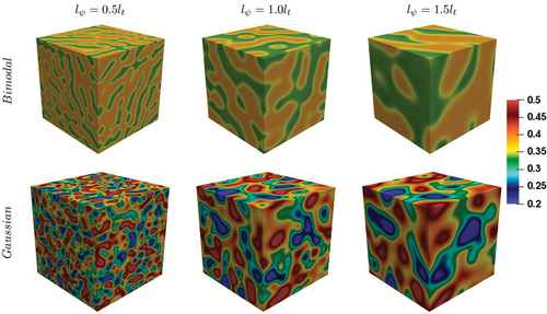
Figure 1. Variations of ${\psi }^f$ at $t=0$ (i.e. initial conditions), for the cases with ${\psi }_{mean}^f=0.356$ and ${\sigma }_f^{{\psi }^f}=0.05$, for $l_{\psi }=0.5l_t,1.0l_t$ and 1$.5l_t$ (left to right), for both bimodal and Gaussian initial distributions (top to bottom) as indicated by the respective labels.

The mean dilution level considered here falls within the range considered in previous experimental analyses (Galmiche et al. 2011; Larsson, Berg, Bonaldo 2013). A diffusion timescale can be estimated as t_diff ~λ²_Ψ/D (where ${\lambda }_{\psi }$ is the Taylor-micro scale of $\mathrm{C}{\mathrm{O}}_2$ inhomogeneity) varies between $50t_{sp}-300t_{sp}$ for $l_{\psi }=0.5l_t$ to $1.5l_t$, respectively. This indicates that the $\mathrm{C}{\mathrm{O}}_2$ inhomogeneity survives during the course of the simulation for all cases considered here.

The initial bimodal and Gaussian distributions of the mixture composition have been chosen in such a manner to mimic real-life biogas combustors, and engine modifications widely used in eastern Europe, India and Bangladesh to utilize biogas instead of petroleum-based fuels due to its availability and low cost (Koonaphapdeelert, Aggarangsi, Moran 2020; Korberg, Skov, Mathiesen 2020; Mustafi and Agarwal 2020; Patterson et al. 2011; Rafiee et al. 2021). The overall composition of the biogas may be controlled (i.e. ${\psi }_{mean}^f$) but the fuel composition supplied to the fuel injectors might not be perfectly homogeneous (i.e. ${\sigma }_f^{{\psi }^f}\ne 0$) giving rise to different initial ‘dilution distributions’ which the present study attempts to mimic.

RESULTS & DISCUSSION

It is important to discuss the scope of this study prior to interpreting the results. As mentioned in the introduction, extensive experimental and computational studies have been carried out into the investigation of premixed (uniform spatial distribution) biogas mixtures. As existing studies have focused on the variation of the level of $\mathrm{C}{\mathrm{O}}_2$ present in the mixture, the effects arising from an increase in the $\mathrm{C}{\mathrm{O}}_2$ content of the fuel mixture are well-known (Galmiche et al. 2011; Larsson, Berg, Bonaldo 2013). An increase of the level of $\mathrm{C}{\mathrm{O}}_2$ serves to decrease the burning rate of the mixture, and the maximum values of temperature and fuel reaction rate magnitude, and is detrimental toward obtaining successful combustion. The present study principally focuses on the effects arising from the variation of the initial spatial distributions (uniform, bimodal and Gaussian) and not the effects arising from the variation of mean carbon dioxide content and initial turbulence intensity. This analysis aims to reveal how the variation of the spatial distribution of $\mathrm{C}{\mathrm{O}}_2$ can affect the evolution of the hot gas kernel initiated by thermal runaway by comparing the differing initial spatial distributions of $\mathrm{C}{\mathrm{O}}_2$ (Gaussian and bimodal distribution). Thus, it is instructive to first inspect the variation in the mixture composition encountered between the different initial spatial distributions under initial conditions (see Figure 1) and also its evolution when the flame kernel is established as a result of localized forced ignition. For this purpose the isosurfaces of $c=0.85$ at $t=6.0t_{sp}$ for initial $u{ }^{\mathrm{\prime }}/s_l^0=8.0$ and ${\psi }_{mean}^f=0.356$ for the homogeneous mixture and inhomogeneous bimodal and Gaussian distribution cases corresponding to initial ${\sigma }_f^{{\psi }^f}=0.07$ and $l_{\psi }=1.5l_t$ are exemplarily presented in Figure 2. The translucent pink sphere in Figure 2 indicates the energy deposition volume with a radius of $R_{sp}$. To allow for inspection of the mixture composition, which is encountered by the flame kernel, planes in all three directions at a perpendicular distance of 11${\delta }_z^0$ from the center of the domain colored by ${\psi }^f$ are shown. As Figure 2 presents the behavior at $t=6.0t_{sp}$, turbulence has been able to aid the mixing of $\mathrm{C}{\mathrm{O}}_2$. 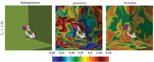Despite the high value of initial turbulence intensity, the mixture composition remains significantly different between the cases shown and the influence of the inhomogeneous $\mathrm{C}{\mathrm{O}}_2$ distribution is still visible, even at this advanced time. However, despite the significantly different mixture compositions encountered by the hot gas kernel across the different initial spatial distributions, the shapes of the isosurfaces remain similar but have some minor differences. The most noticeable of these is present for the initial bimodal distribution, as the tendril of the isosurface closest to the spark volume, has separated from the rest of the hot gas kernel for these cases whilst this behavior is not present for the other cases. This behavior is attributed to the dominant effects arising from the high initial turbulence intensity, which primarily governs the shape of the hot gas kernel and the same initial turbulent velocity field is used for all these cases. Secondly, the amount of energy being deposited into the mixture is the same across all initial distributions, and is also significantly higher than the corresponding MIE for the perfectly premixed diluted mixture (Galmiche et al. 2011; Larsson, Berg, Bonaldo 2013; Turquand d’Auzay et al. 2019a). Thus, the deposited energy is enough to ensure a successful thermal runaway for this level of mean dilution. The dominant effects of flame wrinkling and mixing driven by initial turbulence intensity alongside the deposited energy being greater than the MIE give rise to similar flame shapes across the different initial distributions shown in Figure 2.

Figure 2. Isosurfaces of c$=0.85$ at $t=6.0t_{sp}$ for initial $u{ }^{\mathrm{\prime }}/s_l^0=8.0$ and ${\psi }_{mean}^f=0.356$ for the perfectly homogeneous (1^st column), inhomogeneous spatial distributions of CO₂ dilution following initially Gaussian (2^nd column) and bimodal (3^rd column) distributions with initial. $l_{\psi }=1.5l_{\mathrm{t}}$ $\mathrm{a}\mathrm{n}\mathrm{d}$ ${\sigma }_f^{{\psi }^f}=0.07$. The translucent pink sphere indicates the energy deposition volume. The surfaces showing the local distribution of ${\psi }^f$ are situated at a perpendicular distance of 11${\delta }_z^0$ from the center of the domain.

The temporal evolutions of the maximum values of nondimensional temperature $T=\left(\hat{T}-T_0\right)/\left(T_{ad}^0-T_0\right)$ (i.e. $T_{max}$) and the normalized maximum methane reaction rate magnitude ${\left|{\dot{\omega }}_{C{H}_4}\right|}_{max}\times {\delta }_z^0/{\rho }_0{s}_l^0$ (referred to as ${\left|{\dot{\omega }}_{C{H}_4}\right|}_{max}^{+}$ for brevity) for all the laminar cases with ${\psi }_{mean}^f=0.212$ and ${\sigma }_f^{{\psi }^f}=\hspace{0.17em}$0.07, across all initial spatial distributions are shown in Figure 3a 3b, respectively. The cases shown below are representative of the behavior which is observed across all the parametric variations investigated in the present study, and the trends outlined here hold across all values of parameters investigated. As mentioned earlier, increases in initial turbulence intensity and mean level of dilution act to decrease $T_{max}$ and ${\left|{\dot{\omega }}_{C{H}_4}\right|}_{max}^{+}$ and thus are not explicitly shown here and interested readers are directed to Turquand d’Auzay et al. (2019a) for further detail on these effects. It can be observed from Figure 3a that a near collapse between the profiles of the maximum temperature and reaction rate for all three different initial distributions are present but there are some subtle differences.

Figure 3. Temporal evolution of $T_{max}$ (top row) and for ${\left|{\dot{\omega }}_{C{H}_4}\right|}_{max}^{+}$(bottom row) for initial $l_{\psi }=0.5l_t,1.0l_t$ and 1$.5l_t$ (a-c) as indicated by the respective labels, under laminar conditions for cases with ${\psi }_{mean}^f=0.212$ and initial ${\sigma }_f^{{\psi }^f}=0.07$. Green indicates Gaussian, blue indicates bimodal, and red indicates Uniform, initial spatial distributions of $\mathrm{C}{\mathrm{O}}_2$, respectively. Magenta indicates the corresponding undiluted mixture (${\psi }^f=0.0$). Circle markers indicate cases with non-uniform spatial distribution, whilst square markers indicate cases with uniform spatial distribution (i.e. perfectly homogeneous mixture), to help with readability.

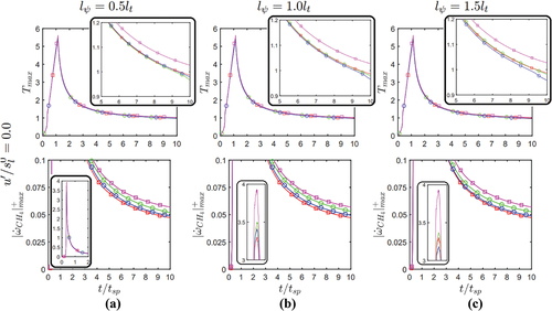
The $T_{max}$ profiles for the Gaussian initial distributions remain near identical to that of the homogeneous mixture regardless of the length scale, however the bimodal distribution displays slightly smaller values of maximum temperature as the length scale increases, with the difference becoming more visible as time advances. However, the normalized reaction rates exhibit an opposite trend to that observed for the temperature profiles, as the maximum normalized reaction rate observed increases from the uniform to the bimodal to the Gaussian initial distribution. To understand why such a behavior is observed, it is useful to refer back to Figure 1 and 2, which indicate that under the inhomogeneous distribution of $\mathrm{C}{\mathrm{O}}_2$ the hot gas kernel can locally encounter pockets of undiluted mixture (pure $\mathrm{C}{\mathrm{H}}_4$), giving rise to the higher maximum value of ${\left|{\dot{\omega }}_{C{H}_4}\right|}_{max}^{+}$ than obtained in the case of uniform distribution of diluent. Moreover, heat is transferred from the zones of high fuel reaction rate magnitude to the neighborhood zones with smaller reaction rate magnitude for inhomogeneous distributions of ${\psi }^f$, which also acts to reduce the corresponding $T_{max}$ value. It is worth noting that the maximum values presented in Figure 3 provide information at a given point in the domain, and thus they have limited significance on the overall burning behavior. Additionally, as can be seen from Figure 3, the differences in the profiles observed are small, and for the turbulent cases, which are not shown here, the profiles completely collapse upon one another. As the effects arising from the variation of the initial distribution as a whole cannot be interpreted from the variations shown in Figure 3, it is useful to inspect the probability density functions (PDFs) of ${\left|{\dot{\omega }}_{C{H}_4}\right|}^{+}$ for the region corresponding to $0.5\le c\le 0.95$ (i.e. reaction zone for the present thermo-chemistry) at $t=5.0t_{sp}$ for all the cases with ${\psi }_{mean}^f=0.212$ and $0.356$ with initial ${\sigma }_f^{{\psi }^f}=\hspace{0.17em}$0.07, which are shown in Figure 4.

Figure 4. PDFs of ${\left|{\dot{\omega }}_{C{H}_4}\right|}^{+}$ for the region corresponding to $0.5\le c\le 0.95$ extracted at $t=5.0t_{sp}$for initial $u{ }^{\mathrm{\prime }}/s_l^0=0,4.0$ and $8.0$ (top to bottom), and initial $l_{\psi }=0.5l_t,1.0l_t$ and 1$.5l_t$ (left to right) as indicated by the respective labels, for the cases with initial ${\sigma }_f^{{\psi }^f}=0.07$, with the solid lines indicating ${\psi }_{mean}^{\mathrm{f}}=0.212$ and the dashed lines indicating ${\psi }_{mean}^{\mathrm{f}}=0.356$. Green indicates Gaussian, blue indicates bimodal, and red indicates Uniform, initial spatial distributions of $\mathrm{C}{\mathrm{O}}_2$, respectively.

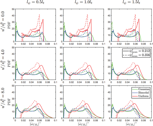
An increase in ${\psi }_{mean}^{\mathrm{f}}$ (solid to dashed lines) leads to a decrease of the probability of finding a large magnitude of ${\left|{\dot{\omega }}_{C{H}_4}\right|}^{+}$ in accordance with pevious findings (Galmiche et al. 2011; Larsson, Berg, Bonaldo 2013; Turquand d’Auzay et al. 2019a). Moving from left to right, implying an increase of $l_{\psi }$, reveals that the PDFs of ${\left|{\dot{\omega }}_{C{H}_4}\right|}^{+}$ are only marginally affected by the variation of $l_{\psi }$ within the parameter range considered here. It was also found that the variation of ${\sigma }_f^{{\psi }^f}$ had no substantial effect and thus those cases are not shown in Figure 4 for the sake of conciseness. The similarity of the PDFs with the variations of both $l_{\psi }$ and ${\sigma }_f^{{\psi }^f}$ are consistent with the findings from Figure 2 and 3. Of particular interest, however, is the spread and distribution of the values of ${\left|{\dot{\omega }}_{C{H}_4}\right|}^{+}$ across the different initial spatial distributions. Differences in the profiles of the PDFs across the Gaussian and bimodal distributions are observed, specifically at the tails of the PDFs. Across all cases, a larger spread of values of ${\left|{\dot{\omega }}_{C{H}_4}\right|}^{+}$ are observed for the initial Gaussian distributions of $\mathrm{C}{\mathrm{O}}_2$ dilution compared to the initial bimodal distributions, and this arises due to the nature of the distributions. As can be seen from Figure 1 and 2, the range of values of ${\psi }^f$ present for the Gaussian initial distribution is larger than that for the bimodal initial distribution, which drives the larger spread of values of ${\left|{\dot{\omega }}_{C{H}_4}\right|}^{+}$ observed for the Gaussian distribution. As expected, the homogeneous distribution displays the smallest range of ${\left|{\dot{\omega }}_{C{H}_4}\right|}^{+}$ values and a range of values of ${\left|{\dot{\omega }}_{C{H}_4}\right|}^{+}$in these cases is obtained due to the variations of $c$ and $T$ within the range of reaction progress variable considered in Figure 4. For both Gaussian and bimodal distributions, the kernel can also locally encounter mixtures with ${\psi }^f>{\psi }_{mean}^{\mathrm{f}}$ which in turn give rise to low values of ${\left|{\dot{\omega }}_{C{H}_4}\right|}^{+}$. As the range of values of ${\psi }^f$, which can be encountered locally under the bimodal conditions, is more restricted than those which can be found for the initial Gaussian distribution of $\mathrm{C}{\mathrm{O}}_2$ dilution, sharper peaks of the PDFs of ${\left|{\dot{\omega }}_{C{H}_4}\right|}^{+}$ are observed for bimodal cases than in the corresponding initial Gaussian distributions. These peaks are not present for the uniform mixture, as for the homogeneous mixture cases with ${\psi }^f={\psi }_{mean}^{\mathrm{f}}$.

In order to fully explain the behavior of the peaks of the PDFs for ${\left|{\dot{\omega }}_{C{H}_4}\right|}^{+}<0.01$, and the similarity of the profiles of the PDFs for ${\left|{\dot{\omega }}_{C{H}_4}\right|}^{+}>0.01$ for both Gaussian and bimodal distributions of $\mathrm{C}{\mathrm{O}}_2$ dilution, the PDFs of ${\psi }^f$ in the unburned mixture (i.e. $T\le 0.01$) and preheat zone (i.e. $0.05\le T\le 0.45$) at three time instants ($t=2.0$,5.0 and 8.0$t_{sp}$) have been exemplarily shown in Figure 5 and 6, respectively for ${\psi }_{mean}^{\mathrm{f}}=0.356$ in the case of initial ${\sigma }_f^{{\psi }^f}=0.07$. 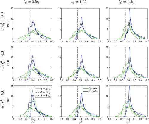The same qualitative behavior has been observed for the other values of mean dilution and variance across both the Gaussian and bimodal initial distributions of $\mathrm{C}{\mathrm{O}}_2$ dilution, and thus they are not shown here for the sake of clarity. Across all cases, the PDFs of ${\psi }^f$ become increasingly narrow with peaks converging around their respective ${\psi }_{mean}^{\mathrm{f}}$ values as time advances due to mixing. Mixing is primarily driven by the effects of turbulence, and also by the integral length scale of the spatial distribution of $\mathrm{C}{\mathrm{O}}_2$. It is worthwhile to start by inspecting the laminar cases to allow for the effects arising from the increase of $l_{\psi }$ in the unburnt mixture to be highlighted, due to the absence of turbulence. For $l_{\psi }=0.5l_t$, both Gaussian and bimodal distributions of $\mathrm{C}{\mathrm{O}}_2$ dilution converge toward a distribution with a peak at their respective mean values, and this behavior is more visible for the bimodal distribution. However, for $l_{\psi }=1.0l_t$, both Gaussian and bimodal distributions retain some resemblance to their initial profiles throughout the duration of the simulation time. Lastly, for $l_{\psi }=1.5l_t$, the PDFs of ${\psi }^f$ broaden indicating that a wider range of values of ${\psi }^f$ can potentially be encountered in the unburned gas for both Gaussian and bimodal distributions. The rate of mixing increases with increasing initial $u{ }^{\mathrm{\prime }}/s_l^0$ and thus the distribution of ${\psi }^f$ in the unburned gas becomes increasingly narrow with a peak at ${\psi }^{\mathrm{f}}\approx {\psi }_{mean}^{\mathrm{f}}$ as time advances with an increase in $u{ }^{\mathrm{\prime }}/s_l^0$. Although the mixture is stoichiometric (i.e. $\xi ={\xi }_{st}$) everywhere in the domain, both $\xi$ and ${\xi }_{st}$ exhibit spatial variations due to the inhomogeneous distribution of ${\psi }^f$. Thus, the integral length scale of ${\psi }^f$ provides a measure of the scalar dissipation rate of mixture fraction $N_{\xi }$ such that a small value of $l_{\psi }$ yields large values of $N_{\xi }$ (Patel and Chakraborty 2014, 2016a). As a result, a decrease in $l_{\psi }$ acts to increase the mixing of $\mathrm{C}{\mathrm{O}}_2$ in the unburned gas. For the large value of $l_{\psi }=1.5l_t$, the mixing rate of $\mathrm{C}{\mathrm{O}}_2$ dilution is relatively small and thus the diffusion of $\mathrm{C}{\mathrm{O}}_2$ produced as a result of the chemical reaction into the unburned gas acts to slightly increase the range of value of ${\psi }^f$ encountered in the unburned mixture, as time advances. This is responsible for the observed broadening of ${\psi }^{\mathrm{f}}$ PDFs with time in Figure 5 for initial $l_{\psi }=1.5l_t$ but the rate of mixing of $\mathrm{C}{\mathrm{O}}_2$ is faster for smaller values of $l_{\psi }$ and thus the PDFs of ${\psi }^{\mathrm{f}}$ narrow with time for initial $l_{\psi }=0.5l_t$ and $l_{\psi }=1.0l_t$ cases. The trend described above in terms of $l_{\psi }$ for laminar cases is also present in the turbulent cases, however it is not as visible due to the mixing induced from the effects of turbulence. As initial turbulence intensity increases, so too does the rate of mixing, as evidenced by the faster narrowing of the PDFs around the initial mean ${\psi }^f$values.

Figure 5. PDFs of ${\psi }^f$ evaluated for the unburned mixture (i.e. $T\le 0.01$) at $t=2.0t_{sp}$ (solid lines), $t=5.0t_{sp}$ (dashed lines) and $t=8.0t_{sp}$ (dotted lines with circle markers) for both initial Gaussian (green) and bimodal (blue) distributions for ${\psi }_{mean}^f=0.356$ with initial ${\sigma }_f^{{\psi }^f}=0.07$ for initial $u{ }^{\mathrm{\prime }}/s_l^0=0,4.0$ and $8.0$ (top to bottom), and initial $l_{\psi }=0.5l_t,1.0l_t$ and 1$.5l_t$ (left to right) as indicated by the respective labels. The vertical dashed lines indicate ${\psi }_{mean}^f=0.356$.

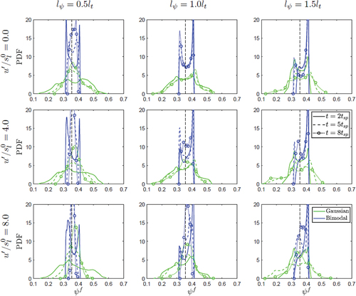
Figure 6. PDFs of ${\psi }^f$ evaluated for the preheat zone (i.e. $0.05\le T\le 0.45$) at $t=2.0t_{sp}$ (solid lines), $t=5.0t_{sp}$ (dashed lines) and $t=8.0t_{sp}$ (dotted lines with circle markers) for both initial Gaussian (green) and bimodal (blue) distributions for ${\psi }_{mean}^f=0.356$ with ${\sigma }_f^{{\psi }^f}=0.07$ for initial $u{ }^{\mathrm{\prime }}/s_l^0=0,4.0$ and $8.0$ (top to bottom), and initial $l_{\psi }=0.5l_t,1.0l_t$ and 1$.5l_t$ (left to right) as indicated by the respective labels. The vertical dashed lines indicate ${\psi }_{mean}^f=0.356$.

At this point, it is worth recalling that Figure 2 and 3 demonstrate that the differences between the results obtained for bimodal and Gaussian distributions of$\mathrm{C}{\mathrm{O}}_2$ dilution are marginal, despite the significant differences in both initial conditions and the mixture composition encountered by the kernels during its evolution. In order to understand this behavior, it is worthwhile to consider the PDFs shown in Figure 6.

The PDFs of Figure 6 suggest that the most probable mixture composition in the preheat zone of the hot gas kernel is almost the same for both Gaussian and bimodal distributions of $\mathrm{C}{\mathrm{O}}_2$ dilution, and this tendency strengthens as time advances. At $t=8.0t_{sp}$, the PDFs of ${\psi }^f$ for both initial Gaussian and bimodal distribution cases become similar due to turbulent and molecular mixing occurring in the unburned mixture, as explained previously. For the homogeneous $\mathrm{C}{\mathrm{O}}_2$ distribution, the hot gas kernel always interacts with mixtures with a dilution level of ${\psi }^f={\psi }_{mean}^f$. However, in the case of non-uniform spatial $\mathrm{C}{\mathrm{O}}_2$ distributions, the probabilities of finding ${\psi }^f>{\psi }_{mean}^f$ increase for $0.05\le T\le 0.45$. The samples corresponding to $0.05\le T\le 0.45$ include different values of $c$. The mixture composition corresponding to ${\psi }^f<{\psi }_{mean}^f$ burns faster and attains higher burned gas temperatures and higher $c$ values. Thus, the low temperature slow burning regions (e.g. $0.05\le T\le 0.45$) predominantly include samples from high $\mathrm{C}{\mathrm{O}}_2$ dilution leading to a mean ${\psi }^f$, which is greater than ${\psi }_{mean}^f$. This also explains why the cases with a non-uniform spatial distribution of $\mathrm{C}{\mathrm{O}}_2$ exhibit different ${\left|{\dot{\omega }}_{C{H}_4}\right|}^{+}$ statistics to that in the case of the homogeneous mixtures (see Figure 4), but also as to why similar behavior is observed in spite of the significantly different initial conditions arising from the Gaussian and bimodal initial distributions of $\mathrm{C}{\mathrm{O}}_2$ dilution. It can further be seen from Fig, 6 that the range of values of ${\psi }^f$ which the flame kernel encounters are much more limited for the bimodal distribution than those with an initial Gaussian initial $\mathrm{C}{\mathrm{O}}_2$ distribution. Thus, the probability of finding small values of ${\left|{\dot{\omega }}_{C{H}_4}\right|}^{+}$ is higher for the case of initial Gaussian distribution than in the case of initial bimodal distribution.

In this analysis, three statistically independent realizations for the parameters listed in Table 2 were used to analyze the stochastic effects. Due to a large number of cases, only the cases with initial ${\sigma }_f^{{\psi }^f}=0.07$ for ${\psi }_{mean}^f=0.212$ and 0.356 are presented for the sake of conciseness. In order to illustrate the effects arising from stochastic effects, the temporal evolutions of the mean volume of the region with $c\ge 0.9$ (i.e. 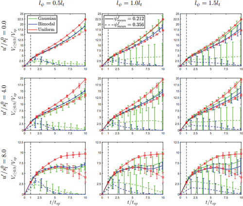$V_{c\ge 0.9}$), normalized by $V_{sp}=4\pi R_{sp}^3/3$ are shown in Figure 7, with the error bars indicating the standard deviation based on all three realizations, at that given time. Figure 7 demonstrates that $V_{c\ge 0.9}/V_{sp}$ decreases with increasing ${\psi }_{mean}^f$ (solid to dashed lines) for a given $u{ }^{\mathrm{\prime }}/s_l^0$, which is consistent with previous experimental (Galmiche et al. 2011; Larsson, Berg, Bonaldo 2013) and computational (Turquand d’Auzay et al. 2019a) findings. An increase in initial turbulence intensity acts to increase the turbulent eddy diffusivity D_t~u'l_t and thus enhances the heat transfer rate from the hot gas kernel, and acts to reduce the burned gas volume, which is consistent with several previous analyses (Chakraborty, Cant, Mastorakos 2007; Chakraborty and Mastorakos 2008; Chakraborty, Hesse, Mastorakos 2010; Wandel, Chakraborty, Mastorakos 2009; Patel and Chakraborty 2014, 2015, 2016a-c; Turquand d’Auzay et al. 2019a,b). The growth of the hot gas kernel depends on the competition between the heat release rate and heat transfer rate from the hot gas kernel. An increase in $\mathrm{C}{\mathrm{O}}_2$ dilution reduces the burning rate and thus heat release also decreases, which leads to a reduction in $V_{c\ge 0.9}/V_{sp}$ with increasing ${\psi }_{mean}^f$.

Figure 7. Temporal evolutions of mean $V_{c\ge 0.9}/V_{sp}$ with initial ${\sigma }_f^{{\psi }^f}=0.07$ for ${\psi }_{mean}^f=0.212$ (solid lines) and ${\psi }_{mean}^f=0.356$ (dashed lines), for initial $u{ }^{\mathrm{\prime }}/s_l^0=0,4.0$ and $8.0$ (top to bottom) and initial $l_{\psi }=0.5l_t,1.0l_t$ and 1$.5l_t$ (left to right) as indicated by the respective labels. Blue indicates bimodal, green indicates Gaussian, and red indicates uniform initial spatial distributions of $\mathrm{C}{\mathrm{O}}_2$, respectively. The lines indicate the mean value of $V_{c\ge 0.9}/V_{sp}$ at that time instant across all three realizations investigated, whilst the error bars indicate the standard deviation. All cases shown in this figure have an initial value of ${\sigma }_f^{\psi }=0.07$.

To be able to fully understand the influence of the multiple parameters which play a role in determining the outcome of the localized forced ignition, it is instructive to inspect the two different levels of ${\psi }_{mean}^f$ separately. For the cases with ${\psi }_{mean}^f=0.212$ (solid lines) the standard deviation of $V_{c\ge 0.9}/V_{sp}$, as indicated by the error bars, is significantly smaller than the standard deviation observed for the ${\psi }_{mean}^f=0.356$ cases. The MIE for biogas increases with increasing ${\psi }_{mean}^f$ (Galmiche et al. 2011; Larsson, Berg, Bonaldo 2013) and thus for a given amount of input energy, the ratio of the deposited energy to the corresponding MIE is greater in the ${\psi }_{mean}^f=0.212$ cases than in the ${\psi }_{mean}^f=0.356$ cases. Observing the uniform distributions (red lines) for $u{ }^{\mathrm{\prime }}/s_l^0=8.0$ (bottom row), it can be seen that for ${\psi }_{mean}^f=0.212$ (solid lines), successful propagation (defined as a positive temporal derivative of $V_{c\ge 0.9}/V_{sp}$ at the end of the simulation) is obtained in a mean sense. This is not the case for the equivalent ${\psi }_{mean}^f=0.356$ (dashed lines) cases, as the profiles are indicative of flame quenching in a mean sense. An increase in initial turbulence intensity has similar effects to those outlined for an increase of ${\psi }_{mean}^f$ and the same reasoning regarding the relative magnitude of the deposited energy in comparison to the corresponding MIE applies here due to the increasing trend of the MIE with an increase in $u{ }^{\mathrm{\prime }}/s_l^0$ (Galmiche et al. 2011; Larsson, Berg, Bonaldo 2013).

An increase of $l_{\psi }$ (moving left to right), is found to be beneficial for obtaining self-sustained propagation for the hot gas kernels resulting from localized ignition. The slow mixing rate for higher values of $l_{\psi }$ increases the probability of finding ${\psi }^f<{\psi }_{mean}^f$ and the rate of heat release is higher for mixtures with smaller $\mathrm{C}{\mathrm{O}}_2$ dilution levels. Thus, the heat release rate from the hot gas kernel counters the heat transfer from it more effectively for a higher value of $l_{\psi }$. This is best highlighted by the turbulent cases (bottom two rows) with ${\psi }_{mean}^f=0.356$ (dashed lines) where quenching of the flame kernel occurs at a later time as $l_{\psi }$ increases for both the bimodal and Gaussian initial distributions.

Additionally, an increase of $l_{\psi }$ also serves to increase the variability of the outcomes observed (i.e. larger standard deviations), and this can best be seen for the laminar cases (top row) with ${\psi }_{mean}^f=0.212$ (solid lines). As outlined in the context of Figure 5 and 6, a decrease in the value of $l_{\psi }$ serves to increase the rate of mixing, and thus the effects arising from the differing initial distributions of $\mathrm{C}{\mathrm{O}}_2$ dilution between the different realizations disappear earlier for smaller values of $l_{\psi }$ due to the faster rate of mixing.

Lastly and most importantly, the effects of the different initial $\mathrm{C}{\mathrm{O}}_2$ dilution distributions need to be understood. As expected, the homogeneous $\mathrm{C}{\mathrm{O}}_2$ distribution has the least amount of variability in its outcomes, and the variability in the outcome in these cases is induced solely by the different turbulent realizations. A comparison of the outcomes for initially Gaussian and bimodal spatial distributions of $\mathrm{C}{\mathrm{O}}_2$ reveals that the variability of the outcome for the bimodal distribution is smaller than that in the case of Gaussian distribution. This occurs due to the smaller range of ${\psi }^f$ values in the bimodal distribution as opposed to the Gaussian distribution, as shown previously in Figure 1, 5, 6. Additionally, a Gaussian distribution is expected to increase the chances of a successful outcome compared to the initial bimodal distribution, as highlighted by the higher mean values of $V_{c\ge 0.9}/V_{sp}$ at later times. It can be surmised from the above findings that a bimodal distribution will allow for more repeatable results in comparison to the Gaussian distribution when the deposited energy is significantly greater than the corresponding MIE value. However, an initial Gaussian distribution increases the likelihood of a successful self-sustained flame propagation following thermal runaway compared to the initial bimodal distribution in cases where successful flame propagation is not ensured due to high levels of ${\psi }_{mean}^f$. To summarize, if a departure from a non-uniform initial spatial distribution of $\mathrm{C}{\mathrm{O}}_2$ is to occur for a given value of ${\psi }_{mean}^f$, it is beneficial to have a combination of large values of $l_{\psi }$, small values of $u{ }^{\mathrm{\prime }}/s_l^0$ and a Gaussian initial distribution of $\mathrm{C}{\mathrm{O}}_2$ in order to increase the probability of a successful self-sustained flame propagation subsequent to thermal runaway as a result of external energy addition. It is important to appreciate that three statistically independent realizations are used in the current analysis as a compromise because of the high computational cost of DNS (altogether 354 simulations are conducted here). However, despite the absence of statistical convergence, these statistically independent realization results show a clear trend, which indicates that high values of $l_{\psi }$, small values of $u{ }^{\mathrm{\prime }}/s_l^0$ for an initially Gaussian distribution of $\mathrm{C}{\mathrm{O}}_2$ increase the chance of successful self-sustained flame propagation following thermal runaway induced by the external energy addition.

CONCLUSIONS

The localized forced ignition and subsequent flame propagation have been analyzed for stoichiometric biogas-air mixtures with three different initial spatial distributions of $\mathrm{C}{\mathrm{O}}_2$ dilution (uniform, bimodal and Gaussian) under different flow conditions (initial $u{ }^{\mathrm{\prime }}/s_l^0=4.0$ and 8.0 in addition to a quiescent laminar flow condition). The initial spatial distributions of $\mathrm{C}{\mathrm{O}}_2$ dilution are characterized by Gaussian and bimodal PDFs with specified values of mean (${\psi }_{mean}^f=0.212,0.356$ and $0.539$), standard deviation (${\sigma }_f^{{\psi }^f}$ = 0.05, 0.07) and integral length scale $l_{\psi }$ ($=0.5l_t,1.0l_t,1.5l_t$). Additionally, perfectly premixed uniformly distributed undiluted (${\psi }_{mean}^f=0$) and diluted stoichiometric methane-air mixtures (equivalent to the uniform initial conditions) have been considered for each different initial flow condition for the purpose of comparison with the ignition characteristics of stoichiometric biogas-air mixtures.

It has been found that non-uniform $\mathrm{C}{\mathrm{O}}_2$ dilution has a marginal effect on the shape of the flame kernel, and on the temporal evolutions of the maximum values of burned gas temperature and fuel (i.e. $\mathrm{C}{\mathrm{H}}_4$) reaction rate magnitude in biogas-air mixtures, irrespective of the nature of the initial spatial distribution of $\mathrm{C}{\mathrm{O}}_2$ dilution. Additionally, a departure from uniform $\mathrm{C}{\mathrm{O}}_2$ dilution leads to a larger range of values of the consumption rate of the fuel (i.e. $\mathrm{C}{\mathrm{H}}_4$) than that observed for the homogeneous $\mathrm{C}{\mathrm{O}}_2$ dilution distribution. A Gaussian initial distribution gives rise to higher values of the consumption rate of the fuel compared to the bimodal initial distribution of dilution. The variations of ${\sigma }_f^{{\psi }^f}$ and $l_{\psi }$ (i.e. the characteristics of the initial distribution) have been found to have marginal influence on the consumption rate of the fuel. The increases of ${\psi }_{mean}^f$ and $u{ }^{\mathrm{\prime }}/s_l^0$ have been found to have detrimental effects on the consumption rate of the fuel.

The variations of $l_{\psi }$ considered here have been found to influence the level of mixing in the unburned gas, with a decrease in $l_{\psi }$ acting to increase the rate of mixing. An increase of initial $u{ }^{\mathrm{\prime }}/s_l^0$ has also been found to aid the rate of mixing in the unburned gas. The initial bimodal distribution of $\mathrm{C}{\mathrm{O}}_2$ has been found to mix more rapidly and converge toward a uniform dilution distribution corresponding to ${\psi }_{mean}^f$ faster than the initial Gaussian $\mathrm{C}{\mathrm{O}}_2$ distribution for the unburned mixture. The initial Gaussian distribution of $\mathrm{C}{\mathrm{O}}_2$ dilution leads to a non-negligible possibility of the kernel encountering mixtures with ${\psi }^f<{\psi }_{mean}^f$, unlike in the initial bimodal $\mathrm{C}{\mathrm{O}}_2$ distribution. Thus, the cases with initial Gaussian distribution of $\mathrm{C}{\mathrm{O}}_2$ dilution exhibit higher likelihood of obtaining a successful self-sustained flame propagation than the bimodal initial distribution. The variation of${\sigma }_f^{{\psi }^f}$ within the parameter range considered in the present study has been found to have a marginal influence due to the dominant effects arising from $l_{\psi }$ and $u{ }^{\mathrm{\prime }}/s_l^0$.

The stochastic effects of different initial turbulence and $\mathrm{C}{\mathrm{O}}_2$ dilution distributions have also been analyzed in detail. An increase in ${\psi }_{mean}^f$ and$l_{\psi }$ was found to increase the variability of the burned gas mass, with an increase of $l_{\psi }$ also increasing the variability of a successful thermal runaway and subsequent self-sustained propagation being obtained across all initial spatial distributions. Although the variation of ${\sigma }_f^{{\psi }^f}$ for a given value of ${\psi }_{mean}^f$ has been found to have a marginal influence, the non-zero values of $l_{\psi }$ and ${\sigma }_f^{{\psi }^f}$ (i.e. departure from uniform conditions) have been found to be detrimental for burning rate and decrease the chances of a successful ignition and subsequent self-sustained flame propagation. Due to the multiple parameters investigated in this study and their interaction with each other, it is useful to list them in terms of their importance. The most significant effects were found to arise from the variations of ${\psi }_{mean}^f$ and initial $u{ }^{\mathrm{\prime }}/s_l^0$. An increase of both parameters led to a higher variability of the outcome observed, along with a decrease in the probability of a successful event being observed. The variations of the initial distributions of $\mathrm{C}{\mathrm{O}}_2$ and $l_{\psi }$ have been found to have secondary effects on the localized forced ignition of biogas-air mixtures. The ignition outcomes in the case of homogeneous $\mathrm{C}{\mathrm{O}}_2$ distributions have been found to be the most repeatable, and these cases exhibit a high likelihood of successful ignition events. Both the bimodal and Gaussian distributions of $\mathrm{C}{\mathrm{O}}_2$ dilution in the unburned gas have been found to increase the variability of the outcomes, leading to a higher probability of flame extinction. However, it was found that the Gaussian distribution performed better than the bimodal distribution in terms of successful outcomes of the ignition event. An increase of $l_{\psi }$ leads to a higher probability of obtaining successful events in a mean sense, and the physical reasons for this behavior have been explained in terms of the effects of $l_{\psi }$ on the rate of mixing of $\mathrm{C}{\mathrm{O}}_2$. Lastly, the variations of ${\sigma }_f^{{\psi }^f}$ were found to have a negligible effect on the rate of burning for the range of parameters considered here. The present findings indicate that if a departure from a perfect premixing (i.e. homogeneous distribution) is to occur, a roughly Gaussian profile (e.g. diffusion from a point source) of $\mathrm{C}{\mathrm{O}}_2$ dilution has been found to increase the probability of a successful self-sustained flame propagation subsequent to thermal runaway induced by external energy addition in comparison to that a bimodal $\mathrm{C}{\mathrm{O}}_2$ dilution distribution for a given set of values of ${\sigma }_f^{\psi },l_{\psi }$, ${\psi }_{mean}^f$ and $u{ }^{\mathrm{\prime }}/s_l^0$.

It is important to note that the present analysis has been conducted for a two-step chemical mechanism in the interest of computational economy for a detailed parameteric analysis. Moreover, the simulations have been conducted in a canonical configuration and thus the results obtained here are of qualitative significance. Therefore, future analyses using three-dimensional DNS with detailed chemistry and transport, which is capable of predicting both the flame propagation and ignition delay accurately, will be necessary for further validation. Moreover, the present analysis has been conducted for decaying turbulence but this may not be true in actual IC engines and thus this analysis should also be conducted under forced turbulence to ascertain if any aspects of the current findings alter in the presence of forced turbulence.

Acknowledgments

The financial support of the British Council and EPSRC (EP/R029369/1) and the computational support of Rocket and ARCHER are gratefully acknowledged.

Correction Statement

This article has been republished with minor changes. These changes do not impact the academic content of the article.

Additional information

Funding

This work was supported by the Engineering and Physical Sciences Research Council [EP/R029369/1].

References

- Aspden, A. J. 2017. A numerical study of diffusive effects in turbulent lean premixed hydrogen flames. Proc. Combust. Inst. 36 (2):1997–2004. doi:10.1016/j.proci.2016.07.053.
- Bachelor, G. K., and A. A. Townsend. 1948. Decay of turbulence in final period. Proc. R.Soc. Lond. A194:527–43.
- Ballal, D. R., and A. H. Lefebvre. 1975. The influence of flow parameters on minimum ignition energy and quenching distances. Proc. Combust. Inst. 15 (1):1473–81. doi:10.1016/S0082-0784(75)80405-X.
- Ballal, D. R., and A. H. Lefebvre. 1977. Spark ignition of turbulent flowing gases, 129–55. Reston, VA: 15th Aerospace Sciences Meeting, 155, American Institute of Aeronautics and Astronautics.
- Bansal, G., and H. G. Im. 2011. Autoignition and front propagation in low temperature combustion environments. Combust. Flame 158 (11):2105–12. doi:10.1016/j.combustflame.2011.03.019.
- Barik, D., and S. Murugan. 2014. Investigation on combustion performance and emission characteristics of a DI (direct injection) diesel engine fueled with biogas diesel in dual fuel mode. Energy 72:760–71. doi:10.1016/j.energy.2014.05.106.
- Bibrzycki, J., and T. Poinsot, 2010, Reduced chemical kinetic mechanisms for methane combustion in O2/N2 and O2/CO2 atmosphere, Work. note ECCOMET WN/CFD/10/17, CERFACS.
- Bilger, R. 1980. Turbulent flows with nonpremixed reactants. In Turbulent Reacting Flows, ed. P. Libby and F. Williams., Vol. 44 of Topics in Applied Physics, 65–113. Berlin/Heidelberg: Springer.
- Boree, J., and P. C. Miles. 2014. Cylinder Flow, Encyclopedia of Automotive Engineering. London, UK: John Wiley & Sons. doi:10.1002/9781118354179.
- Cardin, C., B. Renou, G. Cabot, and A. M. Boukhalfa. 2013a. Experimental analysis of laserinduced spark ignition of lean turbulent premixed flames: New insight into ignition transition. Combust. Flame 160 (8):1414–27. doi:10.1016/j.combustflame.2013.02.026.
- Cardin, C., B. Renou, G. Cabot, and A. M. Boukhalfa. 2013b. Experimental analysis of laserinduced spark ignition of lean turbulent premixed flames. Comptes Rendus Mécanique 341 (1–2):191–200. doi:10.1016/j.crme.2012.10.019.
- Chakraborty, N., R. S. Cant, and E. Mastorakos. 2007. Effects of turbulence on spark ignition in inhomogeneous mixtures: A Direct Numerical Simulation (DNS) study. Combust. Sci. Technol. 179:293–317.
- Chakraborty, N., H. Hesse, and E. Mastorakos. 2010. Effects on fuel Lewis number on localised forced ignition of turbulent mixing layers. Flow Turb. Combust 84:125–66.
- Chakraborty, N., and E. Mastorakos. 2006. Numerical Investigation of edge flame propagation characteristics in turbulent mixing layers. Phys. Fluids 18 (10):105103. doi:10.1063/1.2357972.
- Chakraborty, N., and E. Mastorakos. 2008. Direct Numerical Simulation of localised forced ignition of turbulent mixing layers: The effects of mixture fraction and its gradient. Flow Turb. Combust. 80:155–86.
- Champion, M., B. Deshaies, G. Joulin, and K. Kinoshita. 1986. Spherical flame initiation: Theory versus experiments for lean propane air mixtures. Combustion and Flame 65 (3):319–37. doi:10.1016/0010-2180(86)90045-3.
- Chen, J. H., A. Choudhary, D. De Supinski, E. R. Hawkes, S. Klasky, W. K. Liao, K. L. Ma, J. Mellor-Crummey, N. Podhorski, R. Sankaran, et al. 2009. Terascale direct numerical simulations of turbulent combustion using S3D. Comput Sci. Discovery 2 (1):015001.
- Chung, S. H. 2007. Stabilization, propagation and instability of tribrachial triple flames. Proc. Combust. Inst. 31 (1):877–92. doi:10.1016/j.proci.2006.08.117.
- Crookes, R. J. 2006. Comparative bio-fuel performance in internal combustion engines. Biomass Bioenergy 30 (5):461–68. doi:10.1016/j.biombioe.2005.11.022.
- Echekki, T., and J. H. Chen. 1998. Structure and propagation of methanol-air Triple flames. Combust. Flame 114 (1–2):23–245. doi:10.1016/S0010-2180(97)00287-3.
- Espí, C. V., and A. Liñán. 2001. Fast, non-diffusive ignition of a gaseous reacting mixture subject to a point energy source. Combust. Theory Model. 5 (3):485–98. doi:10.1088/1364-7830/5/3/313.
- Espí, C. V., and A. Liñán. 2002. Thermal-diffusive ignition and flame initiation by a local energy source. Combust. Theory Model. 6 (2):297–315. doi:10.1088/1364-7830/6/2/309.
- Eswaran, V., and S. B. Pope. 1988. Direct numerical simulations of the turbulent mixing of a passive scalar. Phys. Fluids 31:506–20.
- EU and Bluesky, 2018, Robust kit to convert diesel vehicles to natural gas and biogas for extended life and reduced contaminants emission, https://trimis.ec.europa.eu/entityprint/node/18812.
- Forsich, C., M. Lackner, F. Winter, H. Kopecek, and E. Wintner. 2004. Characterization of laser-induced ignition of biogas-air mixtures. Biomass Bioenergy 27 (3):299–312. doi:10.1016/j.biombioe.2004.02.002.
- Galmiche, B., F. Halter, F. Foucher, and P. G. Dagaut. 2011. Effects of dilution on laminar burning velocity of premixed methane/air flames. Energy Fuels 25 (3):948–54. doi:10.1021/ef101482d.
- Hawkes, E. R., R. Sankaran, P. Pebay, and J. H. Chen. 2006. Direct numerical simulation of ignition front propagation in a constant volume with temperature inhomogeneities: II. Parametric study. Combustion and Flame 145 (1–2):145–59. doi:10.1016/j.combustflame.2005.09.018.
- He, L. 2000. Critical conditions for spherical flame initiation in mixtures with high Lewis numbers. Combust. Theory Model. 4 (2):159–72. doi:10.1088/1364-7830/4/2/305.
- Heeger, C., B. Bohm, S. F. Ahmed, R. Gordon, I. Boxx, W. Meier, A. Dreizler, and E. Mastorakos. 2009. Statistics of relative and absolute velocities of turbulent non-premixed edge flames following spark ignition. Proc. Combust. Inst. 32 (2):2957–64. doi:10.1016/j.proci.2008.07.006.
- Hesse, H., N. Chakraborty, and E. Mastorakos. 2009. The effects of the Lewis number of the fuel on the displacement speed of edge flames in igniting turbulent mixing layers. Proc. Combust. Inst. 32 (1):1399–407. doi:10.1016/j.proci.2008.06.065.
- Hesse, H., S. P. Malkeson, and N. Chakraborty. 2012. Displacement speed statistics for stratified mixture combustion in an igniting turbulent planar jet. J. Eng. Gas Turbines Power 134 (5):051502. doi:10.1115/1.4005214.
- Im, H. G., and J. H. Chen. 1999. Structure and propagation of triple flames in partially premixed hydrogen-air mixtures. Combust. Flame 119 (4):436–54. doi:10.1016/S0010-2180(99)00073-5.
- Im, H. G., and J. H. Chen. 2001. Effects of flow strain on triple flame propagation. Combust. Flame 126 (1–2):1384–92. doi:10.1016/S0010-2180(01)00261-9.
- Im, H. G., J. H. Chen, and C. K. Law. 1998. Ignition of hydrogen/air mixing layer in turbulent flows. Proc. Combust. Inst. 28 (1):1047–56. doi:10.1016/S0082-0784(98)80505-5.
- IRENA. 2018. Biogas for road vehicles: Technology brief. Abu Dhabi: International Renewable Energy Agency.
- Jatana, G. S., M. Himabindu, H. S. Thakur, and R. V. Ravikrishna. 2014. Strategies for high efficiency and stability in biogas-fuelled small engines. Exper Thermal Fluid Sci. 54:189–95. doi:10.1016/j.expthermflusci.2013.12.008.
- Karami, S., E. R. Hawkes, M. Talei, and J. H. Chen. 2015. Mechanisms of flame stabilisation at low lifted height in a turbulent lifted slot-jet flame. J. Fluid Mech. 777:633–89. doi:10.1017/jfm.2015.334.
- Karami, S., E. R. Hawkes, M. Talei, and J. H. Chen. 2016. Edge flame structure in a turbulent lifted flame: A direct numerical simulation study. Combust. Flame 169:110–28. doi:10.1016/j.combustflame.2016.03.006.
- Ko, Y. S., and S. H. Chung. 1999. Propagation of unsteady tribrachial flames in laminar non-premixed jets. Combust. Flame 118 (1–2):151–63. doi:10.1016/S0010-2180(98)00154-0.
- Koonaphapdeelert, S., P. Aggarangsi, and J. Moran. 2020. Biomethane. In Production and Applications Green Energy and Technology. Singapore: Springer.
- Korberg, A. D., I. R. Skov, and B. V. Mathiesen. 2020. The role of biogas and biogas-derived fuels in a 100% renewable energy system in Denmark. Energy 199:117426. doi:10.1016/j.energy.2020.117426.
- Lafay, Y., B. Taupin, G. Martins, G. Cabot, B. Renou, and A. Boukhalfa. 2007. Experimental study of biogas combustion using a gas turbine configuration, Exp. Fluids 43 (2–3):395–410.
- Larsson, A., A. Berg, and A. Bonaldo. 2013. Fuel flexibility at ignition conditions for industrial gas turbines. Proc. ASME Turbo Expo GT2013–95536.
- Lieuwen, T., V. McDonell, E. Petersen, and D. Santavicca. 2008. Fuel flexibility influences on premixed combustor blowout, flashback autoignition, and stability. J. Eng. Gas Turbines Power 130 (1):810. doi:10.1115/1.2771243.
- Mastorakos, E. 2009. Ignition of turbulent non-premixed flames. Prog. Energy Combust. Sci. 35 (1):57–97.
- Mastorakos, E., T. A. Baritaud, and T. J. Poinsot. 1997. Numerical simulations of autoignition in turbulent mixing flows. Combust. Flame 109 (1–2):198–223. doi:10.1016/S0010-2180(96)00149-6.
- Mordaunt, C. J., and W. C. Pierce. 2014. Design and preliminary results of an atmospheric pressure model gas turbine combustor utilizing varying CO2 doping concentration in CH4 to emulate biogas combustion. Fuel 124:258–68. doi:10.1016/j.fuel.2014.01.097.
- Mulla, I. A., S. R. Chakravarthy, N. Swaminathan, and R. Balachandran. 2016. Evolution of flame-kernel in in laser-induced spark ignited mixtures: A parametric study. Combust. Flame 164:303–18. doi:10.1016/j.combustflame.2015.11.029.
- Mustafi, N. N., and A. K. Agarwal. 2020. Biogas for transport sector: current status, barriers, and path forward for large-scale adaptation. In Alternative Fuels and Their Utilization Strategies in Internal Combustion Engines, Energy, Environment, and Sustainability, ed. A. Singh, Y. Sharma, N. Mustafi, and A. Agarwal. Singapore: Springer.
- Neophytou, A., E. Mastorakos, and R. S. Cant. 2010. DNS of spark ignition and edge flame propagation in turbulent droplet-laden mixing layers. Combust. Flame 157 (6):1071–86. doi:10.1016/j.combustflame.2010.01.019.
- Papacz, W. 2011. Biogas as vehicle fuel. J. KONES Powertrain Transport 18:403–10.
- Papapostolou, V., C. Turquand d’Auzay, and N. Chakraborty. 2020. A numerical investigation of the effects of fuel composition on the minimum ignition energy for homogeneous biogas-air mixtures. Flow Turb. Combust. doi:10.1007/s10494-020-00229-8.
- Papapostolou, V. S., C. Turquand d’ Auzay, G. Ozel-Erol, and N. Chakraborty. 2019. Edge flame propagation statistics in igniting mono-disperse droplet-laden mixtures. Phys. Fluids 31 (10):105108. doi:10.1063/1.5113576.
- Patel, D., and N. Chakraborty. 2014. Localised forced ignition of globally stoichiometric stratified mixtures: A numerical investigation. Combust. Theor. Model. 18 (6):627–51. doi:10.1080/13647830.2014.959456.
- Patel, D., and N. Chakraborty. 2015. Effects of energy deposition characteristics on localised forced ignition of homogeneous mixtures, Int. J. Spray Combust. Dyn. 7 (2):151–74. doi:10.1260/1756-8277.7.2.151.
- Patel, D., and N. Chakraborty. 2016a. Effects of fuel Lewis number on localised forced ignition of globally stoichiometric stratified mixtures: A numerical investigation. Flow Turb. Combust. 96:1083–105.
- Patel, D., and N. Chakraborty. 2016b. Effects of fuel Lewis number and the energy deposition characteristics on localized forced ignition of homogeneous mixture: A numerical investigation. Int. J. Spray Combust. Dyn. 8 (3):183–96. doi:10.1177/1756827716651579.
- Patel, D., and N. Chakraborty. 2016c. Effects of mixture distribution on localised forced ignition of stratified mixtures: A numerical investigation. Combust. Sci. Technol. 188:1904–24.
- Patterson, T., S. Esteves, R. Dinsdale, and A. Guwy. 2011. An evaluation of the policy and techno-economic factors affecting the potential for biogas upgrading for transport fuel use in the UK. Energy Policy 39:1806–16.
- Pera, C., S. Chevillard, and J. Reveillon. 2013. Effect of residual burnt gas heterogeneity on early flame propagation and on cyclic variability in spark-ignited engines. Combust. Flame 160 (6):1020–32. doi:10.1016/j.combustflame.2013.01.009.
- Persson, M. 2007. Biogas upgrading and utilization as vehicle fuel. Proc.Future Biogas Eur III:60–66.
- Poinsot, T., T. Echekki, and M. Mungal. 1992. A study of the laminar flame tip and implications for turbulent premixed combustion. Combust. Sci. Technol. 81 (1–3):45–73. doi:10.1080/00102209208951793.
- Rafiee, A., K. R. Khalilpour, J. Prest, and I. Skryabin. 2021. Biogas as an energy vector. Biomass Bioenergy 144:105935. doi:10.1016/j.biombioe.2020.105935.
- Rasi, S., A. Veijanen, and J. Rintala. 2007. Trace compounds of biogas from different biogas production plants. Energy 32 (8):1375–80. doi:10.1016/j.energy.2006.10.018.
- Ray, J., H. N. Najm, and R. B. McCoy, 2001, Ignition front structure in a methane air jet. Presented at the 2nd Joint Meeting of the U.S. Section of the Combustion Institute, Oakland, California, paper no. 150.
- Rogallo, R. S., 1981, Numerical experiments in homogeneous turbulence. Technical report, NASA Ames, California, USA.
- Ryckebosch, E., M. Drouillon, and H. Vervaeren. 2011. Techniues for transformation of biogas to biomethane. Biomass Bioenergy 35 (5):1633–45. doi:10.1016/j.biombioe.2011.02.033.
- Sankaran, R., H. G. Im, E. R. Hawkes, and J. H. Chen. 2005. The effects of non-uniform temperature distribution on the ignition of a lean homogeneous hydrogen–air mixture, Proc. Combust. Inst. 30 (1):875–82. doi:10.1016/j.proci.2004.08.176.
- Selle, L., G. Lartigue, T. Poinsot, R. Koch, K. U. Schildmacher, W. Krebs, B. Prade, P. Kaufmann, and D. Veynante. 2004. Compressible large eddy simulation of turbulent combustion in complex geometry on unstructured meshes. Combust. Flame 137 (4):489–505. doi:10.1016/j.combustflame.2004.03.008.
- Shah, M. S., P. K. Halder, A. S. M. Shamsuzzaman, M. S. Hossain, S. K. Pal, and E. Sarker. 2017. Perspectives of biogas conversion into Bio-CNG for automobile fuel in Bangladesh. J. Renew. Energy 2017:4385295. doi:10.1155/2017/4385295.
- Sibulkin, M., and K. S. Siskind. 1987. Numerical study of initiation of a combustion wave by an ignition kernel. Combust. Flame 69 (1):49–57. doi:10.1016/0010-2180(87)90020-4.
- Smith, G. P., D. M. Golden, M. Frenklach, N. W. Moriarty, B. Eiteneer, M. Goldenberg, C. T. Bowman, R. K. Hanson, S. Song, W. C. Gardiner, et al., 1995, GRI-MECH 3.0. http://www.me.berkeley.edu/grimech/.
- Smooke, M. D., and V. Giovangigli. 1991. Premixed and nonpremixed test flame results. In Reduced kinetic mechanisms and asymptotic approximations for methane-air flames, 29–47. Berlin: Springer.
- Surataa, I. W., T. G. T. Nindhiab, I. K. A. Atmikac, D. N. K. P. Negarad, and I. W. E. P. Putrae. 2014. Simple conversion method from gasoline to biogas fueled small engine to powered electric generator. Energy Proc. 52:626–32.
- Turquand d’Auzay, C., V. Papapostolou, S. F. Ahmed, and N. Chakraborty. 2019a. Effects of turbulence intensity and biogas composition on the localised forced ignition of turbulent mixing layers. Combust. Sci. Technol. 191:868–97.
- Turquand d’Auzay, C., V. Papapostolou, S. F. Ahmed, and N. Chakraborty. 2019b. On the minimum ignition energy and its transition in the localised forced ignition of turbulent homogeneous mixtures. Combust. Flame 201:104–17. doi:10.1016/j.combustflame.2018.12.015.
- Turquand d’Auzay, C., V. S. Papapostolou, and N. Chakraborty. 2021. Effects of biogas composition on the edge flamepropagation in igniting turbulent mixing layers”. Flow Turb. Combust. 106 (4):1437–59. doi:10.1007/s10494-020-00210-5.
- Vasavan, A., P. De Goey, and J. van Oijen. 2018. Numerical study on the autoignition of biogas in moderate or intense low oxygen dilution nonpremixed combustion systems. Energy Fuels 32 (8):8768–80. doi:10.1021/acs.energyfuels.8b01388.
- Wandel, A. P., N. Chakraborty, and E. Mastorakos. 2009. Direct numerical simulations of turbulent flame expansion in fine sprays. Proc. Combust. Inst. 32 (2):2283–90. doi:10.1016/j.proci.2008.06.102.
- Westbrook, C. K., and F. L. Dryer. 1981. Simplified reaction mechanisms for the oxidation of hydrocarbon fuels in flames. Combust. Sci. Technol. 27 (1–2):31–43. doi:10.1080/00102208108946970.
- Yu, R., and X.-S. Bai. 2010. Direct Numerical Simulation of lean hydrogen/air auto-ignition in a constant volume enclosure. Combust. Flame 157:1071–86.