Sensorless position estimation and control of permanent-magnet synchronous motors using a saturation model

ABSTRACT

Sensorless control of permanent-magnet synchronous motors at low velocity remains a challenging task. A now well-established method consists of injecting a high-frequency signal and using the rotor saliency, both geometric and magnetic-saturation induced. This paper proposes a clear and original analysis based on second-order averaging of how to recover the position information from signal injection; this analysis blends well with a general model of magnetic saturation. It also proposes a simple parametric model of the saturated motor, based on an energy function which simply encompasses saturation and cross-saturation effects. Experimental results on a surface-mounted motor and an interior magnet motor illustrate the relevance of the approach.

KEYWORDS:

• Permanent-magnet synchronous motor (PMSM)
• sensorless control
• signal injection
• magnetic saturation
• energy-based modeling
• second-order averaging

Nomenclature

xij	=	vector made from the real numbers xi and xj, where ij can be dq, αβ or γδ $$x_{ij}:={(x_i,x_j)}^T$$
φij	=	flux linkage due to current
iij	=	stator current
uij	=	impressed voltage
Mμ	=	rotation matrix with angle μ $$M_{\mu }:=\left(\begin{array}{cc}\hfill cos\mu & \hfill -sin\mu \\ \hfill sin\mu & \hfill cos\mu \end{array}\right)$$
$\mathcal{J}$	=	rotation matrix with angle $\frac{\pi }{2}$$$\mathcal{J}:=\left(\begin{array}{cc}\hfill 0& \hfill -1\\ \hfill 1& \hfill 0\end{array}\right)$$
	=	Notice the useful relation $$\frac{d{M}_{\mu }}{d\mu }=\mathcal{J}{M}_{\mu }=M_{\mu }\mathcal{J}$$
λ	=	amplitude of magnet flux
φm	=	constant flux linkage due to permanent magnet $${\phi }_m:={(\lambda ,0)}^T$$
ω	=	rotor (electrical) speed
θ	=	rotor (electrical) position
R	=	stator resistance
n	=	number of pole pairs
J	=	inertia moment (rotor + load)
τL	=	load torque
$\mathcal{H}$	=	magnetic energy function
${\mathcal{I}}_{dq}$	=	nonlinear flux–current relation in the d–q frame
∂k	=	partial derivative with respect to kth variable
D	=	first derivative
Ld, Lq	=	stator inductances
αi, j	=	parameters describing magnetic saturation
$\mathcal{O}$	=	‘Big-O’ symbol of analysis: if f and g are two functions,$f\left(ϵ\right)=\mathcal{O}\left(g\left(ϵ\right)\right)$ means |f(ϵ)| ≤ C|g(ϵ)| for some positive constant C when ϵ → 0
⊙	=	element-wise product of vectors: $x_{ij}\odot y_{ij}:=\left(\begin{array}{c}{x}_i{y}_i\\ x_j{y}_j\end{array}\right)$
θc, η	=	internal states of a general control law
Ω	=	pulsation of fast-varying injected signal
fγδ	=	2π-periodic vector function with zero mean
Fγδ	=	primitive of fγδ with zero mean $$\begin{array}{ccc}\hfill F_{\gamma \delta }\left(\sigma \right)& :=& {\int }_0^{\sigma }{f}_{\gamma \delta }\left(s\right)ds\hfill \\ & & -\frac{1}{2\pi }{\int }_0^{2\pi }{\int }_0^{\sigma }{f}_{\gamma \delta }\left(s\right)dsd\sigma \hfill \end{array}$$
$\bar{x}$	=	‘slowly varying component’ of signal x
$\tilde{x}$	=	amplitude of ‘fast-varying component’ of signal x
$\mathcal{S}(\mu ,i)$	=	‘saliency matrix’ $$\mathcal{S}(\mu ,\bar{i}):=M_{\mu }D{\mathcal{I}}_{dq}\left({\mathcal{I}}_{dq}^{-1}\left(M_{\mu }^{T}i\right)\right)M_{\mu }^T$$

1. Introduction

Permanent-magnet synchronous motors (PMSM) are widely used in industry. In the so-called ‘sensorless’ mode of operation, the rotor position and velocity are not measured and the control law must make do with only current measurements. While sensorless control is well understood at medium to high velocities, it remains a challenging task at low velocity, see, e.g. Delpoux and Floquet (2014) andEzzat, de Leon, and Glumineau (2011). The reason is that observability degenerates at zero velocity, causing a serious problem in the necessary rotor position estimation.

A now well-established method to overcome this problem is to add some persistent excitation by injecting a high-frequency signal, as proposed in Jansen and Lorenz (1995) and use the rotor saliency, whether geometric for interior permanent-magnet machines or induced by main flux saturation for surface permanent-magnet machines, see Ogasawara and Akagi (1998), Corley and Lorenz (1998), Aihara, Toba, Yanase, Mashimo, and Endo (1999), Consoli, Scarcella, and Testa (2001), Ha, Ide, Sawa, and Sul (2003), Jang, Ha, Ohto, Ide, and Sul (2004), Robeischl and Schroedl (2004) and Shinnaka (2008). Three main techniques of signal injection are found in the literature: sinusoidal circular (Bianchi, Fornasiero, & Bolognani, 2011; Consoli et al., 2001; Jansen & Lorenz, 1995; Szalai, Berger, & Petzoldt, 2014; Wang et al., 2014), sinusoidal elliptic (Bolognani, Calligaro, Petrella, & Tursini, 2011; Corley & Lorenz, 1998; Shinnaka, 2008) and sinusoidal pulsating (Ha et al., 2003; Holtz, 2008; Jang et al., 2004; Liu & Zhu, 2014a), where is injected, respectively, a sinusoidal rotating voltage, a sinusoidal elliptic voltage and a sinusoidal pulsating voltage. The position is then estimated from the resulting high-frequency currents, relying on some separation between the high- and low-frequency models of the motor.

Whatever the kind of signal injection used, magnetic (cross)-saturation must moreover be taken into account to get a good position estimation under high-load condition, see Vagati, Pastorelli, and Scapino (2000), De Belie et al. (2005); Holtz (2008), Reigosa, García, Raca, Briz, and Lorenz (2008), Bianchi, Bolognani, and Faggion (2009), De Kock, Kamper, and Kennel (2009), Li, Zhu, Howe, Bingham, and Stone (2009), Sergeant, De Belie, and Melkebeek (2009), Raca, García, Reigosa, Briz, and Lorenz (2010), Bianchi et al. (2011), Zhu and Gong (2011), Sergeant, De Belie, and Melkebeek (2012), Szalai et al. (2014), Wang et al. (2014), Bolognani et al. (2011) and Liu and Zhu (2014a, 2014b). Some model of the saturated PMSM is thus required for a good functioning of a sensorless control law; to be useful it must be rich enough to capture in particular cross-saturation but also simple enough to be used in real-time and to be easily tuned in the field. Saturation can be accurately modeled at the microscopic level by finite element analysis, but this approach is of course unsuitable for real-time operation since it is computationally very heavy and moreover requires a very detailed knowledge of the motor construction; it is used only to validate macroscopic saturation models and to show the impact of saturation on motor operation. For control purposes a cruder but sufficient description of (cross)-saturation at the macroscopic level is used, usually based on flux-current characteristics in the d–q frame. When the currents are used as state variables, this yields an inductance matrix with entries depending on the currents; cross-saturation is accounted for in the off-diagonal entries. Such a saturation model is tuned during a commissioning process, usually with locked-rotor experiments, and later used in real-time during the normal operation of the motor. The (non-measured) fluxes are obtained as functions of the measured currents by open-loop integration of the voltage equations, see Vagati et al. (2000), Guglielmi, Pastorelli, and Vagati (2006), Štumberger, Štumberger, Dolinar, Hamler, and Trlep (2003), and Štumberger, Polajzer, Štumberger, Toman, and Dolinar (2005); alternatively, injection of high-frequency voltages is used, see Ha et al. (2003) and Štumberger et al. (2005).

The contribution of this paper, which builds on the preliminary works of Jebai, Malrait, Martin, and Rouchon (2011, 2012a, 2012b), is twofold: on one hand, we propose a clear and original analysis based on second-order averaging of how to recover the position information from signal injection. This analysis encompasses among others the circular, elliptic and pulsating injection methods; it can accommodate to any form of injected signals, e.g. square signals as in Yoon, Sul, Morimoto, and Ide (2011) and Liu and Zhu (2014b). It also blends well with a general model of magnetic (cross)-saturation. On the other hand, we introduce a simple parametric model of the saturated PMSM, well-adapted to control purposes, based on an energy function which simply takes into account (cross)-saturation effects. It applies to interior magnet PMSM (IPM) and surface-mounted PMSM (SPM) alike. The parameters must be determined beforehand, but we provide a rather simple estimation procedure based on signal injection and linear least squares; the estimation method does not require the knowledge of the stator resistance and is quite insensitive to imperfections of the pulse width modulation (PWM) power stage.

The paper runs as follows. Section 2 presents the saturation model. In Section 3, position estimation by signal injection is studied thanks to second-order averaging. Section 4 is devoted to the estimation of the parameters entering the saturation model, using once again signal injection and averaging. Finally, Section 5 experimentally demonstrates on two kinds of motors (IPM, and SPM with very little geometric saliency) the relevance of the approach and the necessity of considering saturation to correctly estimate the position.

2. An energy-based model of the saturated PMSM

We follow an energy-based approach to derive a parametric model for the saturated PMSM. In full generality, the currents are expressed as partial derivatives of an energy function, see (4(4) $$\begin{array}{c}\hfill i_{dq}={\mathcal{I}}_{dq}\left({\phi }_{dq}\right):=\left(\begin{array}{c}{\partial }_1\mathcal{H}({\phi }_d,{\phi }_q)\hfill \\ {\partial }_2\mathcal{H}({\phi }_d,{\phi }_q)\hfill \end{array}\right),\end{array}$$(4) ), and the electro-magnetic torque as a product of the currents and the flux linkages, see (2(2) $$\begin{array}{c}\hfill \frac{J}{n^2}\frac{d\omega }{dt}=\frac{3}{2}{i}_{dq}^T\mathcal{J}({\phi }_{dq}+{\phi }_m)-\frac{{\tau }_L}{n}\end{array}$$(2) ). That these expressions are indeed valid even in the d–q frame is usually taken for granted, since they mimic the Lagrangian–Hamiltonian formalism, and they of course can be fully justified, see, e.g. Jebai, Combes, Malrait, Martin, and Rouchon (2014).

2.1 Energy-based model

The model of a (three-phase) two-axis PMSM expressed in the synchronous d–q frame reads (see nomenclature for the vector notation x_ij and the definition of the matrices M_θ and $\mathcal{J}$) (1) $$\begin{array}{c}\hfill \frac{d{\phi }_{dq}}{dt}=u_{dq}-R{i}_{dq}-\omega \mathcal{J}({\phi }_{dq}+{\phi }_m)\end{array}$$(1) (2) $$\begin{array}{c}\hfill \frac{J}{n^2}\frac{d\omega }{dt}=\frac{3}{2}{i}_{dq}^T\mathcal{J}({\phi }_{dq}+{\phi }_m)-\frac{{\tau }_L}{n}\end{array}$$(2) (3) $$\begin{array}{c}\hfill \frac{d\theta }{dt}=\omega ,\end{array}$$(3) with φ_dq flux linkage due to the current; φ_m ≔ (λ, 0)^T constant flux linkage due to the permanent magnet; u_dq impressed voltage and i_dq stator current; ω and θ rotor (electrical) speed and position; R stator resistance; n number of pole pairs; J inertia moment and τ_L load torque. The physically impressed voltages are u_αβ ≔ M_θu_dq while the physically measurable currents are i_αβ ≔ M_θi_dq. The current can be expressed in function of the flux linkage thanks to a suitable energy function $\mathcal{H}({\phi }_d,{\phi }_q)$ by (4) $$\begin{array}{c}\hfill i_{dq}={\mathcal{I}}_{dq}\left({\phi }_{dq}\right):=\left(\begin{array}{c}{\partial }_1\mathcal{H}({\phi }_d,{\phi }_q)\hfill \\ {\partial }_2\mathcal{H}({\phi }_d,{\phi }_q)\hfill \end{array}\right),\end{array}$$(4) where ${\partial }_k\mathcal{H}$ denotes the partial derivative with respect to the k^th variable; without loss of generality $\mathcal{H}(0,0)=0$. Such a relation between flux linkage and current naturally encompasses cross-saturation effects.

For an unsaturated PMSM, this energy function reads $$\begin{array}{c}\hfill {\mathcal{H}}_l({\phi }_d,{\phi }_q)=\frac{1}{2L_d}{\phi }_d^2+\frac{1}{2L_q}{\phi }_q^2,\end{array}$$where L_d and L_q are the motor self-inductances, and we recover the usual linear relations $$\begin{array}{ccc}\hfill i_d& =& {\partial }_1{\mathcal{H}}_l({\phi }_d,{\phi }_q)=\frac{{\phi }_d}{L_d}\hfill \\ \hfill i_q& =& {\partial }_2{\mathcal{H}}_l({\phi }_d,{\phi }_q)=\frac{{\phi }_q}{L_q}.\hfill \end{array}$$

Notice the expression for $\mathcal{H}$ should respect the symmetry of the PMSM with respect to the direct axis, i.e. (5) $$\mathcal{H}({\phi }_d,-{\phi }_q)=\mathcal{H}({\phi }_d,{\phi }_q),$$(5) which is obviously the case for ${\mathcal{H}}_l$. Indeed (1(1) $$\begin{array}{c}\hfill \frac{d{\phi }_{dq}}{dt}=u_{dq}-R{i}_{dq}-\omega \mathcal{J}({\phi }_{dq}+{\phi }_m)\end{array}$$(1) )–(3(3) $$\begin{array}{c}\hfill \frac{d\theta }{dt}=\omega ,\end{array}$$(3) ) is left unchanged by the transformation $$\begin{array}{ccc}& & (u_d,u_q,{\phi }_d,{\phi }_q,i_d,i_q,\omega ,\theta ,{\tau }_L)\hfill \\ & & \to (u_d,-u_q,{\phi }_d,-{\phi }_q,i_d,-i_q,-\omega ,-\theta ,-{\tau }_L).\hfill \end{array}$$

2.2 Parametric description of magnetic saturation

Magnetic saturation can be accounted for by considering a more complicated magnetic energy function $\mathcal{H}$, having ${\mathcal{H}}_l$ for quadratic part, but including also higher-order terms. From experiments on several motors (two IPMs and two SPMs with rated powers between 200 and 1500 W, see Section 5.2), we have found saturation effects to be well captured by considering only third- and fourth-order terms; hence $$\begin{array}{ccc}\hfill \mathcal{H}({\phi }_d,{\phi }_q)& =& {\mathcal{H}}_l({\phi }_d,{\phi }_q)+\sum _{i=0}^3{\alpha }_{3-i,i}{\phi }_d^{3-i}{\phi }_q^i\hfill \\ & & +\sum _{i=0}^4{\alpha }_{4-i,i}{\phi }_d^{4-i}{\phi }_q^i.\hfill \end{array}$$This is a perturbative model where the higher-order terms appear as corrections of the dominant term ${\mathcal{H}}_l$. The nine coefficients α_ij together with L_d, L_q are motor dependent. But (5(5) $$\mathcal{H}({\phi }_d,-{\phi }_q)=\mathcal{H}({\phi }_d,{\phi }_q),$$(5) ) implies α_{2, 1} = α_{0, 3} = α_{3, 1} = α_{1, 3} = 0, so that the energy function can be expressed as (6) $$\begin{array}{ccc}\hfill \mathcal{H}({\phi }_d,{\phi }_q)& =& {\mathcal{H}}_l({\phi }_d,{\phi }_q)+{\alpha }_{3,0}{\phi }_d^3+{\alpha }_{1,2}{\phi }_d{\phi }_q^2\hfill \\ & & +{\alpha }_{4,0}{\phi }_d^4+{\alpha }_{2,2}{\phi }_d^2{\phi }_q^2+{\alpha }_{0,4}{\phi }_q^4.\hfill \end{array}$$(6) From (4(4) $$\begin{array}{c}\hfill i_{dq}={\mathcal{I}}_{dq}\left({\phi }_{dq}\right):=\left(\begin{array}{c}{\partial }_1\mathcal{H}({\phi }_d,{\phi }_q)\hfill \\ {\partial }_2\mathcal{H}({\phi }_d,{\phi }_q)\hfill \end{array}\right),\end{array}$$(4) ) and (6(6) $$\begin{array}{ccc}\hfill \mathcal{H}({\phi }_d,{\phi }_q)& =& {\mathcal{H}}_l({\phi }_d,{\phi }_q)+{\alpha }_{3,0}{\phi }_d^3+{\alpha }_{1,2}{\phi }_d{\phi }_q^2\hfill \\ & & +{\alpha }_{4,0}{\phi }_d^4+{\alpha }_{2,2}{\phi }_d^2{\phi }_q^2+{\alpha }_{0,4}{\phi }_q^4.\hfill \end{array}$$(6) ) the currents are then explicitly given by (7) $$\begin{array}{c}\hfill i_d=\frac{{\phi }_d}{L_d}+3{\alpha }_{3,0}{\phi }_d^2+{\alpha }_{1,2}{\phi }_q^2+4{\alpha }_{4,0}{\phi }_d^3+2{\alpha }_{2,2}{\phi }_d{\phi }_q^2\end{array}$$(7) (8) $$\begin{array}{c}\hfill i_q=\frac{{\phi }_q}{L_q}+2{\alpha }_{1,2}{\phi }_d{\phi }_q+2{\alpha }_{2,2}{\phi }_d^2{\phi }_q+4{\alpha }_{0,4}{\phi }_q^3,\end{array}$$(8) which are the so-called flux–current magnetisation curves.

To conclude, the model of the saturated PMSM is given by (1(1) $$\begin{array}{c}\hfill \frac{d{\phi }_{dq}}{dt}=u_{dq}-R{i}_{dq}-\omega \mathcal{J}({\phi }_{dq}+{\phi }_m)\end{array}$$(1) )–(3(3) $$\begin{array}{c}\hfill \frac{d\theta }{dt}=\omega ,\end{array}$$(3) ) and (7(7) $$\begin{array}{c}\hfill i_d=\frac{{\phi }_d}{L_d}+3{\alpha }_{3,0}{\phi }_d^2+{\alpha }_{1,2}{\phi }_q^2+4{\alpha }_{4,0}{\phi }_d^3+2{\alpha }_{2,2}{\phi }_d{\phi }_q^2\end{array}$$(7) )–(8(8) $$\begin{array}{c}\hfill i_q=\frac{{\phi }_q}{L_q}+2{\alpha }_{1,2}{\phi }_d{\phi }_q+2{\alpha }_{2,2}{\phi }_d^2{\phi }_q+4{\alpha }_{0,4}{\phi }_q^3,\end{array}$$(8) ), with φ_d, φ_q, ω, θ as state variables. The magnetic saturation effects are represented by the five parameters α_{3, 0}, α_{1, 2}, α_{4, 0}, α_{2, 2} and α_{0, 4}.

2.3 Model with i_d, i_q as state variables

The model of the PMSM is usually expressed with currents as state variables. This can be achieved here by time differentiating $i_{dq}={\mathcal{I}}_{dq}\left({\phi }_{dq}\right)$, $$\begin{array}{c}\hfill \frac{d{i}_{dq}}{dt}=D{\mathcal{I}}_{dq}\left({\phi }_{dq}\right)\frac{d{\phi }_{dq}}{dt},\end{array}$$where $D{\mathcal{I}}_{dq}$ is the derivative of ${\mathcal{I}}_{dq}$ and $\frac{d{\phi }_{dq}}{dt}$ is given by (1(1) $$\begin{array}{c}\hfill \frac{d{\phi }_{dq}}{dt}=u_{dq}-R{i}_{dq}-\omega \mathcal{J}({\phi }_{dq}+{\phi }_m)\end{array}$$(1) ). Fluxes are then expressed as ${\phi }_{dq}={\mathcal{I}}_{dq}^{-1}\left(i_{dq}\right)$ by inverting the nonlinear relations (7(7) $$\begin{array}{c}\hfill i_d=\frac{{\phi }_d}{L_d}+3{\alpha }_{3,0}{\phi }_d^2+{\alpha }_{1,2}{\phi }_q^2+4{\alpha }_{4,0}{\phi }_d^3+2{\alpha }_{2,2}{\phi }_d{\phi }_q^2\end{array}$$(7) )–(8(8) $$\begin{array}{c}\hfill i_q=\frac{{\phi }_q}{L_q}+2{\alpha }_{1,2}{\phi }_d{\phi }_q+2{\alpha }_{2,2}{\phi }_d^2{\phi }_q+4{\alpha }_{0,4}{\phi }_q^3,\end{array}$$(8) ); rather than performing the exact inversion, we can take advantage of the fact the coefficients α_{i, j} are experimentally small. At first order with respect to the α_{i, j} we have ${\phi }_d=L_d{i}_d+\mathcal{O}\left(\left|{\alpha }_{i,j}\right|\right)$ and ${\phi }_q=L_q{i}_q+\mathcal{O}\left(\left|{\alpha }_{i,j}\right|\right)$; plugging these expressions into (7(7) $$\begin{array}{c}\hfill i_d=\frac{{\phi }_d}{L_d}+3{\alpha }_{3,0}{\phi }_d^2+{\alpha }_{1,2}{\phi }_q^2+4{\alpha }_{4,0}{\phi }_d^3+2{\alpha }_{2,2}{\phi }_d{\phi }_q^2\end{array}$$(7) )–(8(8) $$\begin{array}{c}\hfill i_q=\frac{{\phi }_q}{L_q}+2{\alpha }_{1,2}{\phi }_d{\phi }_q+2{\alpha }_{2,2}{\phi }_d^2{\phi }_q+4{\alpha }_{0,4}{\phi }_q^3,\end{array}$$(8) ) we find, e.g. $$\begin{array}{ccc}\hfill {\phi }_d& =& L_d\left(i_d-3{\alpha }_{3,0}{\phi }_d^2-{\alpha }_{1,2}{\phi }_q^2-4{\alpha }_{4,0}{\phi }_d^3-2{\alpha }_{2,2}{\phi }_d{\phi }_q^2\right)\hfill \\ & =& L_d(i_d-3{\alpha }_{3,0}(L_d{i}_d+\mathcal{O}\left(\right|{\alpha }_{i,j}{\left|\right))}^2\hfill \\ & & -{\alpha }_{1,2}{\left(L_q{i}_q+\mathcal{O}\left(\right|{\alpha }_{i,j}\left|\right)\right)}^2\hfill \\ & & -4{\alpha }_{4,0}{\left(L_d{i}_d+\mathcal{O}\left(\right|{\alpha }_{i,j}\left|\right)\right)}^3\hfill \\ & & -2{\alpha }_{2,2}\left(L_d{i}_d+\mathcal{O}\left(\right|{\alpha }_{i,j}\left|\right)\right){\left(L_q{i}_q+\mathcal{O}\left(\left|{\alpha }_{i,j}\right|\right)\right)}^2)\hfill \\ & =& L_d(i_d-3{\alpha }_{3,0}{L}_d^2{i}_d^2-{\alpha }_{1,2}{L}_q^2{i}_q^2-4{\alpha }_{4,0}{L}_d^3{i}_d^3\hfill \\ & & -2{\alpha }_{2,2}{L}_d{L}_q^2{i}_d{i}_q^2)+{\left(\mathcal{O}\left(\left|{\alpha }_{i,j}\right|\right)\right)}^2.\hfill \end{array}$$Neglecting $\mathcal{O}\left({\left|{\alpha }_{i,j}\right|}^2\right)$ terms we eventually obtain (9) $$\begin{array}{ccc}\hfill {\phi }_d& =& L_d(i_d-3{\alpha }_{3,0}{L}_d^2{i}_d^2-{\alpha }_{1,2}{L}_q^2{i}_q^2\hfill \\ & & -4{\alpha }_{4,0}{L}_d^3{i}_d^3-2{\alpha }_{2,2}{L}_d{L}_q^2{i}_d{i}_q^2)\hfill \end{array}$$(9) (10) $$\begin{array}{ccc}\hfill {\phi }_q& =& L_q(i_q-2{\alpha }_{1,2}{L}_d{L}_q{i}_d{i}_q-2{\alpha }_{2,2}{L}_d^2{L}_q{i}_d^2{i}_q\hfill \\ & & -4{\alpha }_{0,4}{L}_q^3{i}_q^3).\hfill \end{array}$$(10)

Notice the matrix (11) $$\left(\begin{array}{cc}\hfill G_{dd}\left(i_{dq}\right)& \hfill G_{dq}\left(i_{dq}\right)\\ \hfill G_{dq}\left(i_{dq}\right)& \hfill G_{qq}\left(i_{dq}\right)\end{array}\right):=D{\mathcal{I}}_{dq}\left({\mathcal{I}}_{dq}^{-1}\left(i_{dq}\right)\right),$$(11) with coefficients easily found to be $$\begin{array}{ccc}\hfill G_{dd}\left(i_{dq}\right)& =& \frac{1}{L_d}+6{\alpha }_{3,0}{L}_d{i}_d+12{\alpha }_{4,0}{L}_d^2{i}_d^2+2{\alpha }_{2,2}{L}_q^2{i}_q^2\hfill \\ \hfill G_{dq}\left(i_{dq}\right)& =& 2{\alpha }_{1,2}{L}_q{i}_q+4{\alpha }_{2,2}{L}_d{L}_q{i}_d{i}_q\hfill \\ \hfill G_{qq}\left(i_{dq}\right)& =& \frac{1}{L_q}+2{\alpha }_{1,2}{L}_d{i}_d+2{\alpha }_{2,2}{L}_d^2{i}_d^2+12{\alpha }_{0,4}{L}_q^2{i}_q^2,\hfill \end{array}$$is by construction symmetric; indeed, $$\begin{array}{c}\hfill D{\mathcal{I}}_{dq}\left({\phi }_{dq}\right)=\left(\begin{array}{cc}\hfill {\partial }_{11}\mathcal{H}({\phi }_d,{\phi }_q)& \hfill {\partial }_{21}\mathcal{H}({\phi }_d,{\phi }_q)\\ \hfill {\partial }_{12}\mathcal{H}({\phi }_d,{\phi }_q)& \hfill {\partial }_{22}\mathcal{H}({\phi }_d,{\phi }_q)\end{array}\right)\end{array}$$and ${\partial }_{12}\mathcal{H}={\partial }_{21}\mathcal{H}$. Therefore, the inductance matrix (12) $$\begin{array}{cc}\hfill \left(\begin{array}{cc}\hfill L_{dd}\left(i_{dq}\right)& \hfill L_{dq}\left(i_{dq}\right)\\ \hfill L_{dq}\left(i_{dq}\right)& \hfill L_{qq}\left(i_{dq}\right)\end{array}\right):=& {\left(\begin{array}{cc}\hfill G_{dd}\left(i_{dq}\right)& \hfill G_{dq}\left(i_{dq}\right)\\ \hfill G_{dq}\left(i_{dq}\right)& \hfill G_{qq}\left(i_{dq}\right)\end{array}\right)}^{-1}\end{array}$$(12) is also symmetric, though this is not always acknowledged in saturation models encountered in the literature.

3. Position estimation by signal injection

It is easy and well-known to control a PMSM with a ‘sensored’ control law relying on currents and position measurements. Magnetic saturation can usually be ignored even at low velocity, so that the standard model of the motor with linear relations between current and flux linkage can be used; the control law is in effect sufficiently robust to overcome discrepancies due to saturation. As mentioned in the introduction, the situation is entirely different in the case we are interested in, namely ‘sensorless’ control at low velocity; indeed, the rotor position must now be estimated from the measured currents, and it is in general no longer possible to ignore saturation. The idea is to inject a high-frequency signal, which has nearly no effect on the rotor position and velocity but to produce some small oscillations on the currents. An estimate of the rotor position can then be extracted from these oscillations, and used in a control law. In this way, a standard ‘sensored’ control law relying on currents and position measurements can be turned into a ‘sensorless’ law by using the estimated position in place of the measured position.

3.1 Signal injection and averaging

A control law (sensorless or not) for a PMSM is often designed in the so-called γ − δ frame rotating with velocity $\frac{d{\theta }_c}{dt}$ with respect to the stator frame; θ_c is computed in the control law and usually represents a filtered or estimated version of the rotor angle θ. Setting $x_{\gamma \delta }:=M_{\theta -{\theta }_c}{x}_{dq}$, the system equations (1(1) $$\begin{array}{c}\hfill \frac{d{\phi }_{dq}}{dt}=u_{dq}-R{i}_{dq}-\omega \mathcal{J}({\phi }_{dq}+{\phi }_m)\end{array}$$(1) )–(3(3) $$\begin{array}{c}\hfill \frac{d\theta }{dt}=\omega ,\end{array}$$(3) ) read in this frame (13) $$\begin{array}{c}\hfill \frac{d{\phi }_{\gamma \delta }}{dt}=u_{\gamma \delta }-R{i}_{\gamma \delta }-{\omega }_c\mathcal{J}{\phi }_{\gamma \delta }-\omega \mathcal{J}{M}_{\theta -{\theta }_c}{\phi }_m\end{array}$$(13) (14) $$\begin{array}{c}\hfill \frac{J}{n^2}\frac{d\omega }{dt}=\frac{3}{2}{i}_{\gamma \delta }^T\mathcal{J}({\phi }_{\gamma \delta }+M_{\theta -{\theta }_c}{\phi }_m)-\frac{{\tau }_L}{n}\end{array}$$(14) (15) $$\begin{array}{c}\hfill \frac{d\theta }{dt}=\omega ,\end{array}$$(15) where from (7(7) $$\begin{array}{c}\hfill i_d=\frac{{\phi }_d}{L_d}+3{\alpha }_{3,0}{\phi }_d^2+{\alpha }_{1,2}{\phi }_q^2+4{\alpha }_{4,0}{\phi }_d^3+2{\alpha }_{2,2}{\phi }_d{\phi }_q^2\end{array}$$(7) )–(8(8) $$\begin{array}{c}\hfill i_q=\frac{{\phi }_q}{L_q}+2{\alpha }_{1,2}{\phi }_d{\phi }_q+2{\alpha }_{2,2}{\phi }_d^2{\phi }_q+4{\alpha }_{0,4}{\phi }_q^3,\end{array}$$(8) ) currents and fluxes are related by (16) $$i_{\gamma \delta }=M_{\theta -{\theta }_c}{\mathcal{I}}_{dq}\left(M_{\theta -{\theta }_c}^T{\phi }_{\gamma \delta }\right).$$(16) Since θ_c is known (it is computed in Equation (18(18) $$\begin{array}{c}\hfill \frac{d{\theta }_c}{dt}={\omega }_c(y_m,{\theta }_c,\eta ,t)\end{array}$$(18) ) of the controller), u_γδ can be considered as the actually impressed voltages; similarly the currents i_γδ can be considered as measured. A general control law then looks like the dynamic feedback (17) $$\begin{array}{c}\hfill u_{\gamma \delta }={\mathcal{U}}_{\gamma \delta }(y_m,{\theta }_c,\eta ,t)\end{array}$$(17) (18) $$\begin{array}{c}\hfill \frac{d{\theta }_c}{dt}={\omega }_c(y_m,{\theta }_c,\eta ,t)\end{array}$$(18) (19) $$\begin{array}{c}\hfill \frac{d\eta }{dt}=a(y_m,{\theta }_c,\eta ,t),\end{array}$$(19) where θ_c and the vector η are the internal state variables of the controller, and where the functions ${\mathcal{U}}_{\gamma \delta },{\omega }_c,a$ are suitably designed. The vector y_m comprises all the available measurements, and can be any combination of i_γδ, θ, ω; notice that when y_m consists of only (combinations of) the currents i_γδ, (17(17) $$\begin{array}{c}\hfill u_{\gamma \delta }={\mathcal{U}}_{\gamma \delta }(y_m,{\theta }_c,\eta ,t)\end{array}$$(17) )–(19(19) $$\begin{array}{c}\hfill \frac{d\eta }{dt}=a(y_m,{\theta }_c,\eta ,t),\end{array}$$(19) ) is a so-called ‘sensorless’ controller, i.e. does not rely on position nor velocity measurements. In the sequel, we therefore consider with a slight abuse of notation ${\mathcal{U}}_{\gamma \delta },{\omega }_c,a$ to be functions of i_γδ, θ, ω, θ_c, η, t (rather than functions of y_m, θ_c, η, t).

Signal injection then consists in superimposing on some desirable control law (17(17) $$\begin{array}{c}\hfill u_{\gamma \delta }={\mathcal{U}}_{\gamma \delta }(y_m,{\theta }_c,\eta ,t)\end{array}$$(17) )–(19(19) $$\begin{array}{c}\hfill \frac{d\eta }{dt}=a(y_m,{\theta }_c,\eta ,t),\end{array}$$(19) ) a fast-varying pulsating voltage, (20) $$u_{\gamma \delta }={\mathcal{U}}_{\gamma \delta }(i_{\gamma \delta },\theta ,\omega ,{\theta }_c,\eta ,t)+{\tilde{u}}_{\gamma \delta }\odot f_{\gamma \delta }\left(\Omega t\right),$$(20) where f_γδ is a 2π-periodic vector function with zero mean and ${\tilde{u}}_{\gamma \delta }$ could if desired depend on the same arguments as ${\mathcal{U}}_{\gamma \delta }$ (though it is always taken constant in the sequel); we have used the notation ⊙ to denote the element-wise product $${\tilde{u}}_{\gamma \delta }\odot f_{\gamma \delta }\left(\Omega t\right)=\left(\begin{array}{c}{u}_{\gamma }\\ u_{\delta }\end{array}\right)\odot \left(\begin{array}{c}{f}_{\gamma }\left(\Omega t\right)\\ f_{\delta }\left(\Omega t\right)\end{array}\right):=\left(\begin{array}{c}{u}_{\gamma }{f}_{\gamma }\left(\Omega t\right)\\ u_{\delta }{f}_{\delta }\left(\Omega t\right)\end{array}\right).$$The constant pulsation Ω is chosen ‘large’, so that f_γδ(Ωt) can be seen as a ‘fast’ oscillation; typically Ω ≔ 2π × 500 rad/s in the experiments in Section 5. Notice (20) encompasses the various injection schemes considered in the literature.

Of course an injection scheme is interesting only if it can be shown that:

(i)	it does not substantially modify the action of the ‘base’ control law (17(17) $$\begin{array}{c}\hfill u_{\gamma \delta }={\mathcal{U}}_{\gamma \delta }(y_m,{\theta }_c,\eta ,t)\end{array}$$(17) )–(19(19) $$\begin{array}{c}\hfill \frac{d\eta }{dt}=a(y_m,{\theta }_c,\eta ,t),\end{array}$$(19) );
(ii)	it nevertheless adds to the ‘base’ currents some ‘ripples’ containing position information;
(iii)	it provides a means to extract both ripples and base currents from the actual current measurements.

We propose here a mathematically sound way of dealing with these three points based on the theory of averaging. The following theorem formalises (i), and is later used in Section 3.2 to give a precise meaning to (ii); finally, (iii) is handled in Section 3.3.

Theorem 1:

When the modified control law (20) is applied to (13(13) $$\begin{array}{c}\hfill \frac{d{\phi }_{\gamma \delta }}{dt}=u_{\gamma \delta }-R{i}_{\gamma \delta }-{\omega }_c\mathcal{J}{\phi }_{\gamma \delta }-\omega \mathcal{J}{M}_{\theta -{\theta }_c}{\phi }_m\end{array}$$(13) )–(15(15) $$\begin{array}{c}\hfill \frac{d\theta }{dt}=\omega ,\end{array}$$(15) ), the solution of the resulting closed loop system is (21) $$\begin{array}{c}\hfill {\phi }_{\gamma \delta }={\bar{\phi }}_{\gamma \delta }+\frac{{\tilde{u}}_{\gamma \delta }}{\Omega }\odot F_{\gamma \delta }\left(\Omega t\right)+\mathcal{O}\left(\frac{1}{{\Omega }^2}\right)\end{array}$$(21) (22) $$\begin{array}{c}\hfill \theta =\bar{\theta }+\mathcal{O}\left(\frac{1}{{\Omega }^2}\right)\end{array}$$(22) (23) $$\begin{array}{c}\hfill \omega =\bar{\omega }+\mathcal{O}\left(\frac{1}{{\Omega }^2}\right)\end{array}$$(23) (24) $$\begin{array}{c}\hfill {\theta }_c={\bar{\theta }}_c+\mathcal{O}\left(\frac{1}{{\Omega }^2}\right)\end{array}$$(24) (25) $$\begin{array}{c}\hfill \eta =\bar{\eta }+\mathcal{O}\left(\frac{1}{{\Omega }^2}\right),\end{array}$$(25) where $F_{\gamma \delta }\left(\sigma \right):={\int }_0^{\sigma }{f}_{\gamma \delta }\left(s\right)ds-\frac{1}{2\pi }{\int }_0^{2\pi }{\int }_0^{\sigma }{f}_{\gamma \delta }\left(s\right)dsd\sigma$ is the primitive of f_γδ with zero mean (F_γδ is clearly also 2π-periodic); $({\bar{\phi }}_{\gamma \delta },\bar{\theta },\bar{\omega },{\bar{\theta }}_c,\bar{\eta })$ is the ‘slowly varying’ component of (φ_γδ, θ, ω, θ_c, η), i.e. satisfies $$\begin{array}{ccc}\hfill \frac{d{\bar{\phi }}_{\gamma \delta }}{dt}& =& {\bar{u}}_{\gamma \delta }-R{\bar{i}}_{\gamma \delta }-{\bar{\omega }}_c\mathcal{J}{\bar{\phi }}_{\gamma \delta }-\bar{\omega }\mathcal{J}{M}_{\bar{\theta }-{\bar{\theta }}_c}{\phi }_m\hfill \\ \hfill \frac{J}{n^2}\frac{d\bar{\omega }}{dt}& =& \frac{3}{2}{\bar{i}}_{\gamma \delta }^T\mathcal{J}({\bar{\phi }}_{\gamma \delta }+M_{\bar{\theta }-{\bar{\theta }}_c}{\phi }_m)-\frac{{\tau }_L}{n}\hfill \\ \hfill \frac{d\bar{\theta }}{dt}& =& \bar{\omega }\hfill \\ \hfill \frac{d{\bar{\theta }}_c}{dt}& =& {\omega }_c({\bar{i}}_{\gamma \delta },\bar{\theta },\bar{\omega },{\bar{\theta }}_c,\bar{\eta },t)\hfill \\ \hfill \frac{d\bar{\eta }}{dt}& =& a({\bar{i}}_{\gamma \delta },\bar{\theta },\bar{\omega },{\bar{\theta }}_c,\bar{\eta },t),\hfill \end{array}$$where (26) $$\begin{array}{c}\hfill {\bar{i}}_{\gamma \delta }=M_{\bar{\theta }-{\bar{\theta }}_c}{\mathcal{I}}_{dq}\left(M_{\bar{\theta }-{\bar{\theta }}_c}^T{\bar{\phi }}_{\gamma \delta }\right)\end{array}$$(26) (27) $$\begin{array}{c}\hfill {\bar{u}}_{\gamma \delta }={\mathcal{U}}_{\gamma \delta }({\bar{i}}_{\gamma \delta },\bar{\theta },\bar{\omega },{\bar{\theta }}_c,\bar{\eta },t).\end{array}$$(27)

Notice the slowly-varying system defined above is exactly the same as (13(13) $$\begin{array}{c}\hfill \frac{d{\phi }_{\gamma \delta }}{dt}=u_{\gamma \delta }-R{i}_{\gamma \delta }-{\omega }_c\mathcal{J}{\phi }_{\gamma \delta }-\omega \mathcal{J}{M}_{\theta -{\theta }_c}{\phi }_m\end{array}$$(13) )–(15(15) $$\begin{array}{c}\hfill \frac{d\theta }{dt}=\omega ,\end{array}$$(15) ) acted upon by the unmodified control law (17(17) $$\begin{array}{c}\hfill u_{\gamma \delta }={\mathcal{U}}_{\gamma \delta }(y_m,{\theta }_c,\eta ,t)\end{array}$$(17) )–(19(19) $$\begin{array}{c}\hfill \frac{d\eta }{dt}=a(y_m,{\theta }_c,\eta ,t),\end{array}$$(19) ). In other words, adding signal injection:

• has a very small effect of order $\mathcal{O}\left(\frac{1}{{\Omega }^2}\right)$ on the mechanical variables θ, ω and the controller variables θ_c, η;

• has a small effect of order $\mathcal{O}\left(\frac{1}{\Omega }\right)$ on the flux φ_γδ; this effect will be used in the next section to extract the position information from the measured currents.

A practical use of this result is to provide a sensorless control law from a control law with position measurement: indeed, start with a ‘sensored’ control law (17(17) $$\begin{array}{c}\hfill u_{\gamma \delta }={\mathcal{U}}_{\gamma \delta }(y_m,{\theta }_c,\eta ,t)\end{array}$$(17) )–(19(19) $$\begin{array}{c}\hfill \frac{d\eta }{dt}=a(y_m,{\theta }_c,\eta ,t),\end{array}$$(19) ) where y_m ≔ (i_γδ, θ) and add signal injection; then (20(20) $$u_{\gamma \delta }={\mathcal{U}}_{\gamma \delta }(i_{\gamma \delta },\theta ,\omega ,{\theta }_c,\eta ,t)+{\tilde{u}}_{\gamma \delta }\odot f_{\gamma \delta }\left(\Omega t\right),$$(20) )-(18(18) $$\begin{array}{c}\hfill \frac{d{\theta }_c}{dt}={\omega }_c(y_m,{\theta }_c,\eta ,t)\end{array}$$(18) )-(19(19) $$\begin{array}{c}\hfill \frac{d\eta }{dt}=a(y_m,{\theta }_c,\eta ,t),\end{array}$$(19) ) where θ is everywhere replaced by its estimate $\widehat{\theta }$ extracted from the measured currents is a sensorless control law which nearly behaves as the original ‘sensored’ control law.

Proof: The proof relies on a direct application of the theorem of second-order averaging of differential equations, see Sanders, Verhulst, and Murdock (2007) Section 2.9.1 and for the slow-time dependence Section 3.3; see also Mossaheb (1983). Indeed set $ϵ:=\frac{1}{\Omega }$ and x ≔ (φ_γδ, ω, θ, θ_c, η); then (13(13) $$\begin{array}{c}\hfill \frac{d{\phi }_{\gamma \delta }}{dt}=u_{\gamma \delta }-R{i}_{\gamma \delta }-{\omega }_c\mathcal{J}{\phi }_{\gamma \delta }-\omega \mathcal{J}{M}_{\theta -{\theta }_c}{\phi }_m\end{array}$$(13) )–(15(15) $$\begin{array}{c}\hfill \frac{d\theta }{dt}=\omega ,\end{array}$$(15) ) acted upon by the modified control law (20(20) $$u_{\gamma \delta }={\mathcal{U}}_{\gamma \delta }(i_{\gamma \delta },\theta ,\omega ,{\theta }_c,\eta ,t)+{\tilde{u}}_{\gamma \delta }\odot f_{\gamma \delta }\left(\Omega t\right),$$(20) )-(18(18) $$\begin{array}{c}\hfill \frac{d{\theta }_c}{dt}={\omega }_c(y_m,{\theta }_c,\eta ,t)\end{array}$$(18) )-(19(19) $$\begin{array}{c}\hfill \frac{d\eta }{dt}=a(y_m,{\theta }_c,\eta ,t),\end{array}$$(19) ), once written in the ‘slow time’ $\sigma :=\frac{t}{ϵ}$, is in the so-called standard form for averaging (with slow-time dependance) $$\begin{array}{c}\hfill \frac{dx}{d\sigma }=ϵf_1(x,ϵ\sigma ,\sigma ),\end{array}$$with f₁ T-periodic with respect to its third variable (T = 2π in our case) and ϵ as a small parameter. Therefore, its solution can be approximated as $$\begin{array}{c}\hfill x\left(\sigma \right)=z\left(\sigma \right)+ϵ{\xi }_1\left(z\left(\sigma \right),ϵ\sigma ,\sigma \right)+\mathcal{O}\left({ϵ}^2\right),\end{array}$$where z(σ) is the solution of $$\begin{array}{c}\hfill \frac{dz}{d\sigma }=ϵg_1(z,ϵ\sigma )+{ϵ}^2{g}_2(z,ϵ\sigma );\end{array}$$the functions ξ₁, g₁, g₂ are computed as $$\begin{array}{ccc}\hfill g_1(y,ϵ\sigma )& :=& \frac{1}{T}{\int }_0^T{f}_1(y,ϵ\sigma ,s)ds\hfill \\ \hfill {\zeta }_1(y,ϵ\sigma ,\sigma )& :=& {\int }_0^{\sigma }\left(f_1(y,ϵ\sigma ,s)-g_1(y,ϵ\sigma )\right)ds\hfill \\ \hfill {\xi }_1(y,ϵ\sigma ,\sigma )& :=& {\zeta }_1(y,ϵ\sigma ,\sigma )-\frac{1}{T}{\int }_0^T{\zeta }_1(y,ϵ\sigma ,s)ds\hfill \\ \hfill K_2(y,ϵ\sigma ,\sigma )& :=& {\partial }_1{f}_1(y,ϵ\sigma ,\sigma ){\xi }_1(y,ϵ\sigma ,\sigma )\hfill \\ & & -{\partial }_1{\xi }_1(y,ϵ\sigma ,\sigma )g_1(y,ϵ\sigma )\hfill \\ \hfill g_2(y,ϵ\sigma )& :=& \frac{1}{T}{\int }_0^T{K}_2(y,ϵ\sigma ,s)ds.\hfill \end{array}$$In our case the situation is particularly simple since $$f_1(x,ϵ\sigma ,\sigma )={\bar{f}}_1(x,ϵ\sigma )+{\tilde{u}}_{\gamma \delta }{\odot }_0{f}_{\gamma \delta }\left(\sigma \right),$$i.e. the time-varying part is additive with constant coefficients; we have used the notation ⊙₀ to denote the ‘padded’ element-wise product $${\tilde{u}}_{\gamma \delta }{\odot }_0{f}_{\gamma \delta }\left(\Omega t\right):=\left(\begin{array}{c}{\tilde{u}}_{\gamma \delta }\odot f_{\gamma \delta }\left(\Omega t\right)\\ 0_{(dimx-2)\times 1}\end{array}\right),$$i.e. the dimension 2 vector ${\tilde{u}}_{\gamma \delta }\odot f_{\gamma \delta }\left(\Omega t\right)$ padded with enough zeros to get a vector of the same dimension as x. We then find $$\begin{array}{ccc}\hfill g_1(y,ϵ\sigma )& =& {\bar{f}}_1(y,ϵ\sigma )\hfill \\ \hfill {\zeta }_1(y,ϵ\sigma ,\sigma )& =& {\tilde{u}}_{\gamma \delta }{\odot }_0{\int }_0^{\sigma }{f}_{\gamma \delta }\left(s\right)ds\hfill \\ \hfill {\xi }_1(y,ϵ\sigma ,\sigma )& =& {\tilde{u}}_{\gamma \delta }{\odot }_0{F}_{\gamma \delta }\left(\sigma \right)\hfill \\ \hfill K_2(y,ϵ\sigma ,\sigma )& =& {\partial }_1{\bar{f}}_1(y,ϵ\sigma )·\left({\tilde{u}}_{\gamma \delta }{\odot }_0{F}_{\gamma \delta }\left(\sigma \right)\right)\hfill \\ \hfill g_2(y,ϵ\sigma )& =& 0.\hfill \end{array}$$The case with non-constant ${\tilde{u}}_{\gamma \delta }$ is slightly more complicated, see Jebai et al. (2012b). Translating back to the original variables eventually yields the desired result (21(21) $$\begin{array}{c}\hfill {\phi }_{\gamma \delta }={\bar{\phi }}_{\gamma \delta }+\frac{{\tilde{u}}_{\gamma \delta }}{\Omega }\odot F_{\gamma \delta }\left(\Omega t\right)+\mathcal{O}\left(\frac{1}{{\Omega }^2}\right)\end{array}$$(21) )–(25(25) $$\begin{array}{c}\hfill \eta =\bar{\eta }+\mathcal{O}\left(\frac{1}{{\Omega }^2}\right),\end{array}$$(25) ).

3.2 Position estimation

We now express the effect of signal injection on the currents: plugging (21(21) $$\begin{array}{c}\hfill {\phi }_{\gamma \delta }={\bar{\phi }}_{\gamma \delta }+\frac{{\tilde{u}}_{\gamma \delta }}{\Omega }\odot F_{\gamma \delta }\left(\Omega t\right)+\mathcal{O}\left(\frac{1}{{\Omega }^2}\right)\end{array}$$(21) ) into (16(16) $$i_{\gamma \delta }=M_{\theta -{\theta }_c}{\mathcal{I}}_{dq}\left(M_{\theta -{\theta }_c}^T{\phi }_{\gamma \delta }\right).$$(16) ) we find (28) $$\begin{array}{ccc}\hfill i_{\gamma \delta }& =& M_{\bar{\theta }-{\bar{\theta }}_c+\mathcal{O}\left(\frac{1}{{\Omega }^2}\right)}{\mathcal{I}}_{dq}\left(M_{\bar{\theta }-{\bar{\theta }}_c+\mathcal{O}\left(\frac{1}{{\Omega }^2}\right)}^T\right({\bar{\phi }}_{\gamma \delta }\hfill \\ & & +\frac{{\tilde{u}}_{\gamma \delta }}{\Omega }\odot F_{\gamma \delta }\left(\Omega t\right)+\mathcal{O}\left(\frac{1}{{\Omega }^2}\right)\left)\right)\hfill \end{array}$$(28) (29) $$\begin{array}{c}\hfill ={\bar{i}}_{\gamma \delta }+{\tilde{i}}_{\gamma \delta }\odot F_{\gamma \delta }\left(\Omega t\right)+\mathcal{O}\left(\frac{1}{{\Omega }^2}\right),\end{array}$$(29) using (26(26) $$\begin{array}{c}\hfill {\bar{i}}_{\gamma \delta }=M_{\bar{\theta }-{\bar{\theta }}_c}{\mathcal{I}}_{dq}\left(M_{\bar{\theta }-{\bar{\theta }}_c}^T{\bar{\phi }}_{\gamma \delta }\right)\end{array}$$(26) ) and a first-order expansion; also (30) $$\begin{array}{ccc}\hfill {\tilde{i}}_{\gamma \delta }& :=& M_{\bar{\theta }-{\bar{\theta }}_c}D{\mathcal{I}}_{dq}\left(M_{\bar{\theta }-{\bar{\theta }}_c}^T{\bar{\phi }}_{\gamma \delta }\right)M_{\bar{\theta }-{\bar{\theta }}_c}^T\frac{{\tilde{u}}_{\gamma \delta }}{\Omega }\hfill \\ & =& \mathcal{S}(\bar{\theta }-{\bar{\theta }}_c,{\bar{i}}_{\gamma \delta })\frac{{\tilde{u}}_{\gamma \delta }}{\Omega },\hfill \end{array}$$(30) where we have defined the ‘saliency matrix’ (31) $$\mathcal{S}(\mu ,{\bar{i}}_{\gamma \delta }):=M_{\mu }D{\mathcal{I}}_{dq}\left({\mathcal{I}}_{dq}^{-1}\left(M_{\mu }^T{\bar{i}}_{\gamma \delta }\right)\right)M_{\mu }^T.$$(31)

We will see in the next section how to recover ${\tilde{i}}_{\gamma \delta }$ and ${\bar{i}}_{\gamma \delta }$ from the measured currents i_γδ. Therefore, (30(30) $$\begin{array}{ccc}\hfill {\tilde{i}}_{\gamma \delta }& :=& M_{\bar{\theta }-{\bar{\theta }}_c}D{\mathcal{I}}_{dq}\left(M_{\bar{\theta }-{\bar{\theta }}_c}^T{\bar{\phi }}_{\gamma \delta }\right)M_{\bar{\theta }-{\bar{\theta }}_c}^T\frac{{\tilde{u}}_{\gamma \delta }}{\Omega }\hfill \\ & =& \mathcal{S}(\bar{\theta }-{\bar{\theta }}_c,{\bar{i}}_{\gamma \delta })\frac{{\tilde{u}}_{\gamma \delta }}{\Omega },\hfill \end{array}$$(30) ) gives two (redundant) relations relating the unknown angle $\bar{\theta }$ to the known variables ${\bar{\theta }}_c,{\tilde{i}}_{dq},{\bar{i}}_{\gamma \delta },{\tilde{u}}_{dq}$, provided the matrix $\mathcal{S}(\bar{\theta }-{\bar{\theta }}_c,{\bar{i}}_{\gamma \delta })$ effectively depends on its first argument. This ‘saliency condition’ is what is needed to ensure nonlinear observability. The explicit expression for $\mathcal{S}$ is obtained thanks to (11(11) $$\left(\begin{array}{cc}\hfill G_{dd}\left(i_{dq}\right)& \hfill G_{dq}\left(i_{dq}\right)\\ \hfill G_{dq}\left(i_{dq}\right)& \hfill G_{qq}\left(i_{dq}\right)\end{array}\right):=D{\mathcal{I}}_{dq}\left({\mathcal{I}}_{dq}^{-1}\left(i_{dq}\right)\right),$$(11) ). In the case of an unsaturated magnetic circuit, this matrix reduces to $$\begin{array}{ccc}& & \mathcal{S}(\mu ,{\bar{i}}_{\gamma \delta })=M_{\mu }\left(\begin{array}{cc}\hfill \frac{1}{L_d}& \hfill 0\\ \hfill 0& \hfill \frac{1}{L_q}\end{array}\right)M_{\mu }^T\hfill \\ & =& \frac{L_d+L_q}{2L_d{L}_q}\left(\begin{array}{cc}\hfill 1+\frac{L_q-L_d}{L_d+L_q}cos2\mu & \hfill \frac{L_q-L_d}{L_d+L_q}sin2\mu \\ \hfill \frac{L_q-L_d}{L_d+L_q}sin2\mu & \hfill 1-\frac{L_q-L_d}{L_d+L_q}cos2\mu \end{array}\right)\hfill \end{array}$$and does not depend on ${\bar{i}}_{\gamma \delta }$; notice this matrix does not depend on its first argument for an unsaturated machine with no geometric saliency. Notice also (30(30) $$\begin{array}{ccc}\hfill {\tilde{i}}_{\gamma \delta }& :=& M_{\bar{\theta }-{\bar{\theta }}_c}D{\mathcal{I}}_{dq}\left(M_{\bar{\theta }-{\bar{\theta }}_c}^T{\bar{\phi }}_{\gamma \delta }\right)M_{\bar{\theta }-{\bar{\theta }}_c}^T\frac{{\tilde{u}}_{\gamma \delta }}{\Omega }\hfill \\ & =& \mathcal{S}(\bar{\theta }-{\bar{\theta }}_c,{\bar{i}}_{\gamma \delta })\frac{{\tilde{u}}_{\gamma \delta }}{\Omega },\hfill \end{array}$$(30) ) defines in that case two solutions on [ − π, π] for the angle $\bar{\theta }$ since $\mathcal{S}(\mu ,{\bar{i}}_{\gamma \delta })$ is actually a function of 2μ; in the saturated case there is generically only one solution, except for some particular values of ${\bar{i}}_{\gamma \delta }$.

There are several ways to extract the rotor angle information from (30(30) $$\begin{array}{ccc}\hfill {\tilde{i}}_{\gamma \delta }& :=& M_{\bar{\theta }-{\bar{\theta }}_c}D{\mathcal{I}}_{dq}\left(M_{\bar{\theta }-{\bar{\theta }}_c}^T{\bar{\phi }}_{\gamma \delta }\right)M_{\bar{\theta }-{\bar{\theta }}_c}^T\frac{{\tilde{u}}_{\gamma \delta }}{\Omega }\hfill \\ & =& \mathcal{S}(\bar{\theta }-{\bar{\theta }}_c,{\bar{i}}_{\gamma \delta })\frac{{\tilde{u}}_{\gamma \delta }}{\Omega },\hfill \end{array}$$(30) ). The simplest one is through a nonlinear least square problem, i.e. to estimate the rotor position as, (32) $$\widehat{\theta }={\theta }_c+arg\underset{\mu \in ]-\pi ,\pi ]}{min}{∥{\tilde{i}}_{\gamma \delta }-\mathcal{S}(\mu ,{\bar{i}}_{\gamma \delta })\frac{{\tilde{u}}_{\gamma \delta }}{\Omega }∥}^2.$$(32) Solving this problem at each time step requires only a few iterations of a standard optimization algorithm when the initial guess is sufficiently close to the minimum. Since i_γδ hardly varies between two steps and ${\tilde{u}}_{\gamma \delta }$ is constant the minimum computed at a time step is a very good guess for the next step (except of course for the initialisation step). This rather crude approach was sufficient to run in real-time on our experimental setup. Better and leaner methods not requiring the explicit computation of the minimum, e.g. Luenberger-type observers, are conceivable but not considered here.

3.3 Current demodulation

To estimate the position from e.g. (32(32) $$\widehat{\theta }={\theta }_c+arg\underset{\mu \in ]-\pi ,\pi ]}{min}{∥{\tilde{i}}_{\gamma \delta }-\mathcal{S}(\mu ,{\bar{i}}_{\gamma \delta })\frac{{\tilde{u}}_{\gamma \delta }}{\Omega }∥}^2.$$(32) ) it is necessary to extract the low- and high-frequency components ${\bar{i}}_{\gamma \delta }$ and ${\tilde{i}}_{\gamma \delta }$ from the measured current i_γδ. Since by (29(29) $$\begin{array}{c}\hfill ={\bar{i}}_{\gamma \delta }+{\tilde{i}}_{\gamma \delta }\odot F_{\gamma \delta }\left(\Omega t\right)+\mathcal{O}\left(\frac{1}{{\Omega }^2}\right),\end{array}$$(29) ) $i_{\gamma \delta }\left(t\right)\approx {\bar{i}}_{\gamma \delta }\left(t\right)+{\tilde{i}}_{\gamma \delta }\left(t\right)\odot F_{\gamma \delta }\left(\Omega t\right)$ with ${\bar{i}}_{\gamma \delta }$ and ${\tilde{i}}_{\gamma \delta }$ by construction nearly constant on one period of F_γδ, we may write (33) $$\begin{array}{c}\hfill {\bar{i}}_{\gamma \delta }\left(t\right)\approx \frac{1}{T}{\int }_{t-T}^t{i}_{\gamma \delta }\left(s\right)ds\end{array}$$(33) (34) $$\begin{array}{c}\hfill {\tilde{i}}_{\gamma }\left(t\right)\approx \frac{{\int }_{t-T}^t{i}_{\gamma }\left(s\right)F_{\gamma }\left(\Omega s\right)ds}{{\int }_0^T{F}_{\gamma }^2\left(\Omega s\right)ds}\end{array}$$(34) (35) $$\begin{array}{c}\hfill {\tilde{i}}_{\delta }\left(t\right)\approx \frac{{\int }_{t-T}^t{i}_{\delta }\left(s\right)F_{\delta }\left(\Omega s\right)ds}{{\int }_0^T{F}_{\delta }^2\left(\Omega s\right)ds},\end{array}$$(35) where $T:=\frac{2\pi }{\Omega }$. Indeed as F_γ is 2π-periodic with zero mean, $$\begin{array}{ccc}\hfill {\int }_{t-T}^t{i}_{\gamma }\left(s\right)ds& \approx & {\bar{i}}_{\gamma }\left(t\right){\int }_{t-T}^{t}ds+{\tilde{i}}_{\gamma }\left(t\right){\int }_{t-T}^t{F}_{\gamma }\left(\Omega s\right)ds\hfill \\ & =& T{\bar{i}}_{\gamma }\left(t\right)\hfill \\ \hfill {\int }_{t-T}^t{i}_{\gamma }\left(s\right)F_{\gamma }\left(\Omega s\right)ds& \approx & {\bar{i}}_{\gamma }\left(t\right){\int }_{t-T}^t{F}_{\gamma }\left(\Omega s\right)ds\hfill \\ & & +{\tilde{i}}_{\gamma }\left(t\right){\int }_{t-T}^t{F}_{\gamma }^2\left(\Omega s\right)ds\hfill \\ & =& {\tilde{i}}_{\gamma }\left(t\right){\int }_0^T{F}_{\gamma }^2\left(\Omega s\right)ds.\hfill \end{array}$$Similar computations yield i_δ and ${\tilde{i}}_{\delta }$.

Notice that since ${\bar{i}}_{\gamma \delta }$ and ${\tilde{i}}_{\gamma \delta }$ are obtained by integration on the short period T, they have very little phase lag and are suitable for use in closed-loop.

3.4 Discussion

The proposed approach provides a complete analysis of signal injection in a rather general framework:

• it clarifies the so-called ‘high-frequency model’ usually based on the steady-state response to sinusoidal excitation of the motor linear equivalent circuit, e.g. Jansen and Lorenz (1995), Jang et al. (2004), or simply taken for granted, e.g. Corley and Lorenz (1998), Raca et al. (2010). Indeed (21(21) $$\begin{array}{c}\hfill {\phi }_{\gamma \delta }={\bar{\phi }}_{\gamma \delta }+\frac{{\tilde{u}}_{\gamma \delta }}{\Omega }\odot F_{\gamma \delta }\left(\Omega t\right)+\mathcal{O}\left(\frac{1}{{\Omega }^2}\right)\end{array}$$(21) ) asserts the high-frequency flux is ${\tilde{\phi }}_{\gamma \delta }=\frac{{\tilde{u}}_{\gamma \delta }}{\Omega }\odot F_{\gamma \delta }\left(\Omega t\right)$, even for nonsinusoidal excitation and in the presence of nonlinearities caused by saturation

• it blends well with a general saturation model and yields a more precise relation for the ‘high-frequency impedance’ used in the literature; compare (30(30) $$\begin{array}{ccc}\hfill {\tilde{i}}_{\gamma \delta }& :=& M_{\bar{\theta }-{\bar{\theta }}_c}D{\mathcal{I}}_{dq}\left(M_{\bar{\theta }-{\bar{\theta }}_c}^T{\bar{\phi }}_{\gamma \delta }\right)M_{\bar{\theta }-{\bar{\theta }}_c}^T\frac{{\tilde{u}}_{\gamma \delta }}{\Omega }\hfill \\ & =& \mathcal{S}(\bar{\theta }-{\bar{\theta }}_c,{\bar{i}}_{\gamma \delta })\frac{{\tilde{u}}_{\gamma \delta }}{\Omega },\hfill \end{array}$$(30) ) with e.g. (9) in Jang et al. (2004), which is derived from a linear analysis even though saturation is considered

• the extraction of the high-frequency currents ${\tilde{i}}_{\gamma \delta }$ from the measured currents thanks to (34(34) $$\begin{array}{c}\hfill {\tilde{i}}_{\gamma }\left(t\right)\approx \frac{{\int }_{t-T}^t{i}_{\gamma }\left(s\right)F_{\gamma }\left(\Omega s\right)ds}{{\int }_0^T{F}_{\gamma }^2\left(\Omega s\right)ds}\end{array}$$(34) )–(35(35) $$\begin{array}{c}\hfill {\tilde{i}}_{\delta }\left(t\right)\approx \frac{{\int }_{t-T}^t{i}_{\delta }\left(s\right)F_{\delta }\left(\Omega s\right)ds}{{\int }_0^T{F}_{\delta }^2\left(\Omega s\right)ds},\end{array}$$(35) ) can be seen as a generalisation to general periodic signals of the heterodyning methods used in the literature, e.g. Corley and Lorenz (1998); it has the advantage of not requiring a low-pass filter since it is based on the ‘phase-exact’ formula (29(29) $$\begin{array}{c}\hfill ={\bar{i}}_{\gamma \delta }+{\tilde{i}}_{\gamma \delta }\odot F_{\gamma \delta }\left(\Omega t\right)+\mathcal{O}\left(\frac{1}{{\Omega }^2}\right),\end{array}$$(29) ).

4. Estimation of magnetic parameters

The seven parameters in the saturation model (7(7) $$\begin{array}{c}\hfill i_d=\frac{{\phi }_d}{L_d}+3{\alpha }_{3,0}{\phi }_d^2+{\alpha }_{1,2}{\phi }_q^2+4{\alpha }_{4,0}{\phi }_d^3+2{\alpha }_{2,2}{\phi }_d{\phi }_q^2\end{array}$$(7) )–(8(8) $$\begin{array}{c}\hfill i_q=\frac{{\phi }_q}{L_q}+2{\alpha }_{1,2}{\phi }_d{\phi }_q+2{\alpha }_{2,2}{\phi }_d^2{\phi }_q+4{\alpha }_{0,4}{\phi }_q^3,\end{array}$$(8) ) must of course be estimated. This can be done with a rather simple procedure also relying on signal injection and averaging. The method does not depend on the stator resistance; it is also quite insensitive to imperfections of the PWM power stage, thanks to the not small injected voltages.

4.1 Principle

The rotor is locked in the position θ ≔ 0, hence the model (1(1) $$\begin{array}{c}\hfill \frac{d{\phi }_{dq}}{dt}=u_{dq}-R{i}_{dq}-\omega \mathcal{J}({\phi }_{dq}+{\phi }_m)\end{array}$$(1) )–(3(3) $$\begin{array}{c}\hfill \frac{d\theta }{dt}=\omega ,\end{array}$$(3) ) reduces to ω = 0 and (36) $$\begin{array}{ccc}\hfill \frac{d{\phi }_{dq}}{dt}& =& u_{dq}-R{i}_{dq},\hfill \end{array}$$(36) with $i_{dq}={\mathcal{I}}_{dq}\left({\phi }_{dq}\right)$. Moreover, u_dq can now be physically impressed and i_dq physically measured.

As in Section 3.1, but now working directly in the d–q frame, we inject a fast-varying pulsating voltage (37) $$\begin{array}{ccc}\hfill u_{dq}& =& {\bar{u}}_{dq}+{\tilde{u}}_{dq}f\left(\Omega t\right),\hfill \end{array}$$(37) with constant ${\bar{u}}_{dq}$ and ${\tilde{u}}_{dq}$. Here f and its zero-mean primitive F are 2π-periodic scalar functions; it is possible to inject as in (20(20) $$u_{\gamma \delta }={\mathcal{U}}_{\gamma \delta }(i_{\gamma \delta },\theta ,\omega ,{\theta }_c,\eta ,t)+{\tilde{u}}_{\gamma \delta }\odot f_{\gamma \delta }\left(\Omega t\right),$$(20) ) different signals on the d and q axes, but we have not used this possibility. The solution of (36(36) $$\begin{array}{ccc}\hfill \frac{d{\phi }_{dq}}{dt}& =& u_{dq}-R{i}_{dq},\hfill \end{array}$$(36) )–(37(37) $$\begin{array}{ccc}\hfill u_{dq}& =& {\bar{u}}_{dq}+{\tilde{u}}_{dq}f\left(\Omega t\right),\hfill \end{array}$$(37) ) is then $$\begin{array}{ccc}\hfill {\phi }_{dq}& =& {\bar{\phi }}_{dq}+\frac{{\tilde{u}}_{dq}}{\Omega }F\left(\Omega t\right)+\mathcal{O}\left(\frac{1}{{\Omega }^2}\right),\hfill \end{array}$$where ${\bar{\phi }}_{dq}$ the ‘slowly-varying’ component of φ_dq, satisfies (38) $$\begin{array}{ccc}\hfill \frac{d{\bar{\phi }}_{dq}}{dt}& =& {\bar{u}}_{dq}-R{\bar{i}}_{dq},\hfill \end{array}$$(38) with ${\bar{i}}_{dq}={\mathcal{I}}_{dq}\left({\bar{\phi }}_{dq}\right)$. Moreover, (30(30) $$\begin{array}{ccc}\hfill {\tilde{i}}_{\gamma \delta }& :=& M_{\bar{\theta }-{\bar{\theta }}_c}D{\mathcal{I}}_{dq}\left(M_{\bar{\theta }-{\bar{\theta }}_c}^T{\bar{\phi }}_{\gamma \delta }\right)M_{\bar{\theta }-{\bar{\theta }}_c}^T\frac{{\tilde{u}}_{\gamma \delta }}{\Omega }\hfill \\ & =& \mathcal{S}(\bar{\theta }-{\bar{\theta }}_c,{\bar{i}}_{\gamma \delta })\frac{{\tilde{u}}_{\gamma \delta }}{\Omega },\hfill \end{array}$$(30) ) now boils down to (39) $$\begin{array}{ccc}\hfill {\tilde{i}}_{dq}& =& D{\mathcal{I}}_{dq}\left({\mathcal{I}}_{dq}^{-1}\left({\bar{i}}_{dq}\right)\right)\frac{{\tilde{u}}_{dq}}{\Omega }.\hfill \end{array}$$(39)

Since ${\bar{u}}_{dq}$ is constant (38(38) $$\begin{array}{ccc}\hfill \frac{d{\bar{\phi }}_{dq}}{dt}& =& {\bar{u}}_{dq}-R{\bar{i}}_{dq},\hfill \end{array}$$(38) ) implies $R{\bar{i}}_{dq}$ tends to ${\bar{u}}_{dq}$, hence after an initial transient ${\bar{i}}_{dq}$ is constant. 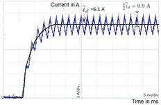As a consequence ${\tilde{i}}_{dq}$ is by (39(39) $$\begin{array}{ccc}\hfill {\tilde{i}}_{dq}& =& D{\mathcal{I}}_{dq}\left({\mathcal{I}}_{dq}^{-1}\left({\bar{i}}_{dq}\right)\right)\frac{{\tilde{u}}_{dq}}{\Omega }.\hfill \end{array}$$(39) ) also constant. Figure 1 shows for instance the time response of i_d for the SPM motor of Section 5 starting from i_d(0) = 0 and using a square function f. As foreseen by the analysis the current ripples recorded on the scope are triangular, with amplitude $\frac{\pi }{2}={max}_{\tau \in [0,2\pi ]}F\left(\tau \right)$ smaller than ${\tilde{i}}_{dq}$ (since f is square with period 2π).

Figure 1. Experimental time response of i_d in (36(36) $$\begin{array}{ccc}\hfill \frac{d{\phi }_{dq}}{dt}& =& u_{dq}-R{i}_{dq},\hfill \end{array}$$(36) )–(37(37) $$\begin{array}{ccc}\hfill u_{dq}& =& {\bar{u}}_{dq}+{\tilde{u}}_{dq}f\left(\Omega t\right),\hfill \end{array}$$(37) ).

The magnetic parameters can then be estimated using (39(39) $$\begin{array}{ccc}\hfill {\tilde{i}}_{dq}& =& D{\mathcal{I}}_{dq}\left({\mathcal{I}}_{dq}^{-1}\left({\bar{i}}_{dq}\right)\right)\frac{{\tilde{u}}_{dq}}{\Omega }.\hfill \end{array}$$(39) ) for various values of ${\bar{u}}_{dq}$ and ${\tilde{u}}_{dq}$, as shown in the next section.

4.2 Estimation of the parameters

From (11(11) $$\left(\begin{array}{cc}\hfill G_{dd}\left(i_{dq}\right)& \hfill G_{dq}\left(i_{dq}\right)\\ \hfill G_{dq}\left(i_{dq}\right)& \hfill G_{qq}\left(i_{dq}\right)\end{array}\right):=D{\mathcal{I}}_{dq}\left({\mathcal{I}}_{dq}^{-1}\left(i_{dq}\right)\right),$$(11) ), the entries of $D{\mathcal{I}}_{dq}\left({\mathcal{I}}_{dq}^{-1}\left({\bar{i}}_{dq}\right)\right)$ are given by $$\begin{array}{ccc}\hfill G_{dd}\left({\bar{i}}_{dq}\right)& =& \frac{1}{L_d}+6{\alpha }_{3,0}{L}_d{\bar{i}}_d+12{\alpha }_{4,0}{L}_d^2{\bar{i}}_d^2+2{\alpha }_{2,2}{L}_q^2{\bar{i}}_q^2\hfill \\ \hfill G_{dq}\left({\bar{i}}_{dq}\right)& =& 2{\alpha }_{1,2}{L}_q{\bar{i}}_q+4{\alpha }_{2,2}{L}_d{\bar{i}}_d{L}_q{\bar{i}}_q\hfill \\ \hfill G_{qq}\left({\bar{i}}_{dq}\right)& =& \frac{1}{L_q}+2{\alpha }_{1,2}{L}_d{\bar{i}}_d+2{\alpha }_{2,2}{L}_d^2{\bar{i}}_d^2+12{\alpha }_{0,4}{L}_q^2{\bar{i}}_q^2.\hfill \end{array}$$Since combinations of the magnetic parameters always enter linearly those equations, they can be estimated by simple linear least squares; moreover, by suitably choosing ${\bar{u}}_{dq}$ and ${\tilde{u}}_{dq}$, the whole least squares problem for the seven parameters can be split into several subproblems involving fewer parameters:

• with ${\bar{u}}_{dq}:=0$, hence ${\bar{i}}_{dq}=0$, (39(39) $$\begin{array}{ccc}\hfill {\tilde{i}}_{dq}& =& D{\mathcal{I}}_{dq}\left({\mathcal{I}}_{dq}^{-1}\left({\bar{i}}_{dq}\right)\right)\frac{{\tilde{u}}_{dq}}{\Omega }.\hfill \end{array}$$(39) ) reads (40) $$\begin{array}{ccc}\hfill L_d& =& \frac{1}{\Omega }\frac{{\tilde{u}}_d}{{\tilde{i}}_d}\hfill \end{array}$$(40) (41) $$\begin{array}{ccc}\hfill L_q& =& \frac{1}{\Omega }\frac{{\tilde{u}}_q}{{\tilde{i}}_q}\hfill \end{array}$$(41)

• with ${\bar{u}}_q=0$, hence ${\bar{i}}_q=0$, and ${\tilde{u}}_q=0$ (39(39) $$\begin{array}{ccc}\hfill {\tilde{i}}_{dq}& =& D{\mathcal{I}}_{dq}\left({\mathcal{I}}_{dq}^{-1}\left({\bar{i}}_{dq}\right)\right)\frac{{\tilde{u}}_{dq}}{\Omega }.\hfill \end{array}$$(39) ) reads (42) $$\begin{array}{ccc}\hfill {\tilde{i}}_d& =& \frac{{\tilde{u}}_d}{\Omega }\left(\frac{1}{L_d}+6{\alpha }_{3,0}{L}_d{\bar{i}}_d+12{\alpha }_{4,0}{L}_d^2{\bar{i}}_d^2\right)\hfill \\ \hfill {\tilde{i}}_q& =& 0,\hfill \end{array}$$(42)

• with ${\bar{u}}_d=0$, hence ${\bar{i}}_d:=0$, and ${\tilde{u}}_q=0$ (39(39) $$\begin{array}{ccc}\hfill {\tilde{i}}_{dq}& =& D{\mathcal{I}}_{dq}\left({\mathcal{I}}_{dq}^{-1}\left({\bar{i}}_{dq}\right)\right)\frac{{\tilde{u}}_{dq}}{\Omega }.\hfill \end{array}$$(39) ) reads (43) $$\begin{array}{c}\hfill {\tilde{i}}_d=\frac{{\tilde{u}}_d}{\Omega }\left(\frac{1}{L_d}+2{\alpha }_{2,2}{L}_q^2{\bar{i}}_q^2\right)\end{array}$$(43) (44) $$\begin{array}{c}\hfill {\tilde{i}}_q=\frac{2{\tilde{u}}_d}{\Omega }{\alpha }_{1,2}{L}_q{\bar{i}}_q,\end{array}$$(44)

• with ${\bar{u}}_d=0$, hence ${\bar{i}}_d:=0$, and ${\tilde{u}}_d=0$ (39(39) $$\begin{array}{ccc}\hfill {\tilde{i}}_{dq}& =& D{\mathcal{I}}_{dq}\left({\mathcal{I}}_{dq}^{-1}\left({\bar{i}}_{dq}\right)\right)\frac{{\tilde{u}}_{dq}}{\Omega }.\hfill \end{array}$$(39) ) reads (45) $$\begin{array}{c}\hfill {\tilde{i}}_d=\frac{2{\tilde{u}}_q}{\Omega }{\alpha }_{1,2}{L}_q{\bar{i}}_q\end{array}$$(45) (46) $$\begin{array}{c}\hfill {\tilde{i}}_q=\frac{{\tilde{u}}_q}{\Omega }\left(\frac{1}{L_q}+12{\alpha }_{0,4}{L}_q^2{\bar{i}}_q^2\right).\end{array}$$(46)

L_d and L_q arethen immediately determined from (40(40) $$\begin{array}{ccc}\hfill L_d& =& \frac{1}{\Omega }\frac{{\tilde{u}}_d}{{\tilde{i}}_d}\hfill \end{array}$$(40) ) and (41(41) $$\begin{array}{ccc}\hfill L_q& =& \frac{1}{\Omega }\frac{{\tilde{u}}_q}{{\tilde{i}}_q}\hfill \end{array}$$(41) ); α_{3, 0} and α_{4, 0} are jointly estimated by least squares from (42(42) $$\begin{array}{ccc}\hfill {\tilde{i}}_d& =& \frac{{\tilde{u}}_d}{\Omega }\left(\frac{1}{L_d}+6{\alpha }_{3,0}{L}_d{\bar{i}}_d+12{\alpha }_{4,0}{L}_d^2{\bar{i}}_d^2\right)\hfill \\ \hfill {\tilde{i}}_q& =& 0,\hfill \end{array}$$(42) ); α_{2, 2}, α_{1, 2} and α_{0, 4} are separately estimated by least squares from, respectively, (43(43) $$\begin{array}{c}\hfill {\tilde{i}}_d=\frac{{\tilde{u}}_d}{\Omega }\left(\frac{1}{L_d}+2{\alpha }_{2,2}{L}_q^2{\bar{i}}_q^2\right)\end{array}$$(43) ), (44(44) $$\begin{array}{c}\hfill {\tilde{i}}_q=\frac{2{\tilde{u}}_d}{\Omega }{\alpha }_{1,2}{L}_q{\bar{i}}_q,\end{array}$$(44) )–(45(45) $$\begin{array}{c}\hfill {\tilde{i}}_d=\frac{2{\tilde{u}}_q}{\Omega }{\alpha }_{1,2}{L}_q{\bar{i}}_q\end{array}$$(45) ) and (46(46) $$\begin{array}{c}\hfill {\tilde{i}}_q=\frac{{\tilde{u}}_q}{\Omega }\left(\frac{1}{L_q}+12{\alpha }_{0,4}{L}_q^2{\bar{i}}_q^2\right).\end{array}$$(46) ), respectively.

5. Experimental results

5.1 Experimental setup

The methodology developed in the paper was tested on two types of motors, an interior magnet PMSM (IPM) and a surface-mounted PMSM (SPM) with very little geometric saliency, with rated parameters listed in the top part of Table 1.

Table 1. Rated and estimated magnetic parameters of test motors.

Motor	IPM	SPM
Rated power	750 W	1500 W
Rated current In (peak)	4.51 A	5.19 A
Rated voltage (peak per phase)	110 V	245 V
Rated speed	1800 rpm	3000 rpm
Rated torque	3.98 Nm	6.06 Nm
n	3	5
R	1.52~Ω	2.1~Ω
λ (peak)	196 mWb	155 mWb
Ld	9.15 mH	7.86 mH
Lq	13.58 mH	8.18 mH
α3, 0L^2dIn	0.039	0.056
α1, 2LdLqIn	0.053	0.055
α4, 0L^3dI^2n	0.0051	0.0164
α2, 2LdL^2qI^2n	0.0171	0.027
α0, 4L^3qI^2n	0.0060	0.0067

The experimental setup consists of an industrial IGBT-inverter (400 V DC bus, 4 kHz PWM frequency), a dSpace fast prototyping system with 3 boards (DS1005, DS5202 and EV1048), and a host computer. The current measurements, used in the sensorless control law, are sampled also at 4 kHz and synchronised with the PWM frequency. The load torque is created by a 4 kW DC motor. For ground truth reference only (i.e. not for use in the sensorless control law), torque and position measurements are available.

5.2 Estimation of the magnetic parameters

We follow the procedure described in Section 4: with the rotor locked in the position θ ≔ 0, a square wave voltage with frequency Ω ≔ 2π × 500 rad/s and constant amplitude ${\tilde{u}}_d$ or ${\tilde{u}}_q$ (15 V for the IPM, 14 V for the SPM) is applied to the motor; but for the determination of L_d, L_q where ${\bar{u}}_d={\bar{u}}_q:=0$, several runs are performed with various ${\bar{u}}_d$ (resp. ${\bar{u}}_q$) such that ${\bar{i}}_d$ (resp. ${\bar{i}}_q$) ranges from −200% to +200% of the rated current. The magnetic parameters are then estimated by linear least squares according to Section 4.2, yielding the values in the bottom part of table 1. Notice the SPM exhibits as expected little geometric saliency (L_d ≈ L_q) hence the saturation-induced saliency is paramount to estimate the rotor position. Notice also the cross-saturation term α₁₂ is as expected quantitatively important for both motors.

The good agreement between the fitted curves and the measurements is demonstrated, for instance, for (42(42) $$\begin{array}{ccc}\hfill {\tilde{i}}_d& =& \frac{{\tilde{u}}_d}{\Omega }\left(\frac{1}{L_d}+6{\alpha }_{3,0}{L}_d{\bar{i}}_d+12{\alpha }_{4,0}{L}_d^2{\bar{i}}_d^2\right)\hfill \\ \hfill {\tilde{i}}_q& =& 0,\hfill \end{array}$$(42) ) and (44(44) $$\begin{array}{c}\hfill {\tilde{i}}_q=\frac{2{\tilde{u}}_d}{\Omega }{\alpha }_{1,2}{L}_q{\bar{i}}_q,\end{array}$$(44) ) in Figures 2 and 3; notice (42(42) $$\begin{array}{ccc}\hfill {\tilde{i}}_d& =& \frac{{\tilde{u}}_d}{\Omega }\left(\frac{1}{L_d}+6{\alpha }_{3,0}{L}_d{\bar{i}}_d+12{\alpha }_{4,0}{L}_d^2{\bar{i}}_d^2\right)\hfill \\ \hfill {\tilde{i}}_q& =& 0,\hfill \end{array}$$(42) ) corresponds to saturation on a single axis while (44(44) $$\begin{array}{c}\hfill {\tilde{i}}_q=\frac{2{\tilde{u}}_d}{\Omega }{\alpha }_{1,2}{L}_q{\bar{i}}_q,\end{array}$$(44) ) corresponds to cross-saturation.

Figure 2. IPM: fitted values vs measurements for (42(42) $$\begin{array}{ccc}\hfill {\tilde{i}}_d& =& \frac{{\tilde{u}}_d}{\Omega }\left(\frac{1}{L_d}+6{\alpha }_{3,0}{L}_d{\bar{i}}_d+12{\alpha }_{4,0}{L}_d^2{\bar{i}}_d^2\right)\hfill \\ \hfill {\tilde{i}}_q& =& 0,\hfill \end{array}$$(42) ) and (44(44) $$\begin{array}{c}\hfill {\tilde{i}}_q=\frac{2{\tilde{u}}_d}{\Omega }{\alpha }_{1,2}{L}_q{\bar{i}}_q,\end{array}$$(44) ).

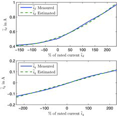
Figure 3. SPM: fitted values vs measurements for (42(42) $$\begin{array}{ccc}\hfill {\tilde{i}}_d& =& \frac{{\tilde{u}}_d}{\Omega }\left(\frac{1}{L_d}+6{\alpha }_{3,0}{L}_d{\bar{i}}_d+12{\alpha }_{4,0}{L}_d^2{\bar{i}}_d^2\right)\hfill \\ \hfill {\tilde{i}}_q& =& 0,\hfill \end{array}$$(42) ) and (44(44) $$\begin{array}{c}\hfill {\tilde{i}}_q=\frac{2{\tilde{u}}_d}{\Omega }{\alpha }_{1,2}{L}_q{\bar{i}}_q,\end{array}$$(44) ).

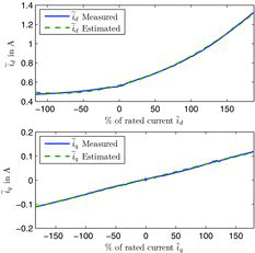
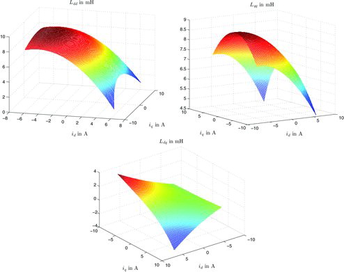
Figure 5 displays the entries of the inductance matrix (12(12) $$\begin{array}{cc}\hfill \left(\begin{array}{cc}\hfill L_{dd}\left(i_{dq}\right)& \hfill L_{dq}\left(i_{dq}\right)\\ \hfill L_{dq}\left(i_{dq}\right)& \hfill L_{qq}\left(i_{dq}\right)\end{array}\right):=& {\left(\begin{array}{cc}\hfill G_{dd}\left(i_{dq}\right)& \hfill G_{dq}\left(i_{dq}\right)\\ \hfill G_{dq}\left(i_{dq}\right)& \hfill G_{qq}\left(i_{dq}\right)\end{array}\right)}^{-1}\end{array}$$(12) ) for the SPM. The importance of (cross)-saturation is well-visible: if the magnetic circuit were linear L_dd, L_qq and L_dq would be planes; if there were no cross-saturation L_dq would be zero.

More thorough tests were conducted on these two motors, as well as on a 200 W IPM and a 1200 W SPM, to fully assess the validity of (6(6) $$\begin{array}{ccc}\hfill \mathcal{H}({\phi }_d,{\phi }_q)& =& {\mathcal{H}}_l({\phi }_d,{\phi }_q)+{\alpha }_{3,0}{\phi }_d^3+{\alpha }_{1,2}{\phi }_d{\phi }_q^2\hfill \\ & & +{\alpha }_{4,0}{\phi }_d^4+{\alpha }_{2,2}{\phi }_d^2{\phi }_q^2+{\alpha }_{0,4}{\phi }_q^4.\hfill \end{array}$$(6) ), see Jebai et al. (2011) for details:

• comparisons between measured and predicted currents ripples when voltages are injected with various angles and magnitudes;

• comparisons between measured and predicted currents time responses on large voltages steps.

5.3 Validation of the rotor position estimation procedure

The relevance of the position estimation methodology developed in Section 3 is now illustrated on the two test motors, using the parameters estimated in the previous section. Following Section 3.1 we start with a standard vector control law (17(17) $$\begin{array}{c}\hfill u_{\gamma \delta }={\mathcal{U}}_{\gamma \delta }(y_m,{\theta }_c,\eta ,t)\end{array}$$(17) )–(19(19) $$\begin{array}{c}\hfill \frac{d\eta }{dt}=a(y_m,{\theta }_c,\eta ,t),\end{array}$$(19) ) where the measurement vector is y_m ≔ (i_γδ, θ). We then addsignal injection (20(20) $$u_{\gamma \delta }={\mathcal{U}}_{\gamma \delta }(i_{\gamma \delta },\theta ,\omega ,{\theta }_c,\eta ,t)+{\tilde{u}}_{\gamma \delta }\odot f_{\gamma \delta }\left(\Omega t\right),$$(20) ), namely ${\tilde{u}}_{\gamma }=15$ V, ${\tilde{u}}_{\delta }=0$, and f_γ a unit square wave with period 2π (f_δ is here irrelevant since u_δ = 0); other injection schemes are of course possible, but notice it is easier to accurately generate square signals than e.g. sinusoidal signals when using as here a PWM stage operating at a rather low frequency. Finally, the estimation $\widehat{\theta }$ is used instead of the measured θ everywhere in (18(18) $$\begin{array}{c}\hfill \frac{d{\theta }_c}{dt}={\omega }_c(y_m,{\theta }_c,\eta ,t)\end{array}$$(18) )–(19(19) $$\begin{array}{c}\hfill \frac{d\eta }{dt}=a(y_m,{\theta }_c,\eta ,t),\end{array}$$(19) )–(20(20) $$u_{\gamma \delta }={\mathcal{U}}_{\gamma \delta }(i_{\gamma \delta },\theta ,\omega ,{\theta }_c,\eta ,t)+{\tilde{u}}_{\gamma \delta }\odot f_{\gamma \delta }\left(\Omega t\right),$$(20) ); $\widehat{\theta }$ is obtained from (32(32) $$\widehat{\theta }={\theta }_c+arg\underset{\mu \in ]-\pi ,\pi ]}{min}{∥{\tilde{i}}_{\gamma \delta }-\mathcal{S}(\mu ,{\bar{i}}_{\gamma \delta })\frac{{\tilde{u}}_{\gamma \delta }}{\Omega }∥}^2.$$(32) ) by a gradient descent algorithm. This indeed results in a sensorless control law relying only on the measured currents, as depicted on Figure 4.

Figure 4. Block diagram of the sensorless control law.

Figure 5. Entries of inductance matrix (12(12) $$\begin{array}{cc}\hfill \left(\begin{array}{cc}\hfill L_{dd}\left(i_{dq}\right)& \hfill L_{dq}\left(i_{dq}\right)\\ \hfill L_{dq}\left(i_{dq}\right)& \hfill L_{qq}\left(i_{dq}\right)\end{array}\right):=& {\left(\begin{array}{cc}\hfill G_{dd}\left(i_{dq}\right)& \hfill G_{dq}\left(i_{dq}\right)\\ \hfill G_{dq}\left(i_{dq}\right)& \hfill G_{qq}\left(i_{dq}\right)\end{array}\right)}^{-1}\end{array}$$(12) ) for SPM.

We stress that the goal of these experiments is to demonstrate the quality of the angle estimation at low speed as well as its usability for closed-loop control, and not the performance of a specific sensorless control law; that is why we have selected a simple base control law for (17(17) $$\begin{array}{c}\hfill u_{\gamma \delta }={\mathcal{U}}_{\gamma \delta }(y_m,{\theta }_c,\eta ,t)\end{array}$$(17) )–(19(19) $$\begin{array}{c}\hfill \frac{d\eta }{dt}=a(y_m,{\theta }_c,\eta ,t),\end{array}$$(19) ).

5.3.1 Long test under various conditions, Figures 6–7

Speed and torque are changed over a period of 210 seconds; the speed remains between ±6% of the rated speed and the torque varies from 0% to 200% of the rated torque. This represents typical operation conditions at low speed. The experimental data on these figures are slightly filtered to be well readable.

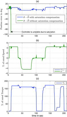
The agreement between the estimated position $\widehat{\theta }$ and the measured position θ when using the saturation model is very good, with an error always smaller than a few (electrical) degrees for the two types of motor. On the contrary, the error on the same experiment when using only the linear model (i.e. with all α_{i, j} zero) is large when the load is high: for the IPM it reaches about 30 (electrical) degrees, Figure 6(a), though the motor is still well-controlled (Figure 6(b) is the same as with the saturation model); for the SPM the error gets so large under high load that the control scheme cannot stabilise the motor, Figure 7(a). This demonstrates the relevance of using the saturation model; in fact it was experimentally noticed that the controller fails to stabilise the motor when the error exceeds about 40 (electrical) degrees.

Figure 6. Long test under various conditions for IPM: (a) position estimation error $\theta -\widehat{\theta }$; (b) measured speed ω (green), reference speed ω_ref (blue); (c) load torque τ_L.

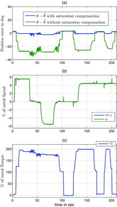
Figure 7. Long test under various conditions for SPM: (a) position estimation error $\theta -\widehat{\theta }$; (b) measured speed ω (green), reference speed ω_ref (blue); (c) load torque τ_L.

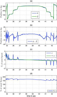
5.3.2 Slow speed reversal, Figures 8–9

This is an excerpt of the long experiment with the saturation model between 40 s and 62 s for the IPM motor and between 34s  and 43s  for the SPM motor. The experimental data are not filtered.

The speed is slowly changed from +0.2% to −0.2% of the rated speed at 180% of the rated torque. This is a very demanding test since the motor always remains in the poor observability region, moreover under high load. Once again the estimated angle closely agrees with the measured angle. The small torque and speed oscillations are caused by the cogging torque and imperfections of the PWM power stage which have a significant effect at very low speed.

Figure 8. Slow speed reversal for IPM: (a) measured θ (blue), estimated $\widehat{\theta }$ (green); (b) position estimation error $\theta -\widehat{\theta }$; (c) measured speed ω (blue), reference speed ω_ref (green); (d) load torque τ_L.

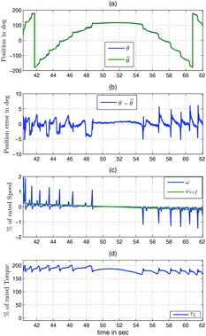
Figure 9. Slow speed reversal for SPM: (a) measured θ (blue), estimated $\widehat{\theta }$ (green); (b) position estimation error $\theta -\widehat{\theta }$; (c) measured speed ω (blue), reference speed ω_ref (green); (d) load torque τ_L.

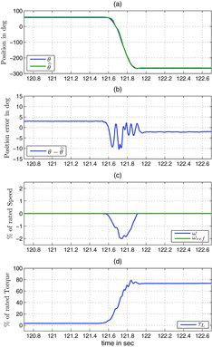
5.3.3 Load step at zero speed, Figures 10–11

This is an excerpt of the long experiment with the saturation model around t = 123 s for the IPM motor and t = 121.5 s for the SPM motor. The experimental data are not filtered.

The load is suddenly changed from 0% to 100% of the rated torque while the motor is at rest. This test illustrates the quality of the estimation also under dynamic conditions.

Figure 10. Load step at zero speed for IPM: (a) measured θ (blue), estimated $\widehat{\theta }$ (green); (b) position estimation error $\theta -\widehat{\theta }$; (c) measured speed ω (blue), reference speed ω_ref; (d) load torque τ_L.

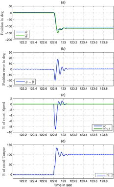
Figure 11. Load step at zero speed for SPM: (a) measured θ (blue), estimated $\widehat{\theta }$ (green); (b) position estimation error $\theta -\widehat{\theta }$; (c) measured speed ω (blue), reference speed ω_ref; (d) load torque τ_L.

5.4 Discussion

The experimental results validate the magnetic saturation model based on the rather simple energy function (6(6) $$\begin{array}{ccc}\hfill \mathcal{H}({\phi }_d,{\phi }_q)& =& {\mathcal{H}}_l({\phi }_d,{\phi }_q)+{\alpha }_{3,0}{\phi }_d^3+{\alpha }_{1,2}{\phi }_d{\phi }_q^2\hfill \\ & & +{\alpha }_{4,0}{\phi }_d^4+{\alpha }_{2,2}{\phi }_d^2{\phi }_q^2+{\alpha }_{0,4}{\phi }_q^4.\hfill \end{array}$$(6) ) depending on the five parameters α_{3, 0}, α_{1, 2}, α_{4, 0}, α_{2, 2}, α_{0, 4} besides the L_d, L_q inductances. They also demonstrate the importance of taking magnetic saturation into account for estimating the rotor position from the measured currents: under high-load condition not considering saturation may lead to estimation errors over 30 (electrical) degrees for an IPM and 80 (electrical) degrees for a SPM, see Figures 6–7, and for more detailed experimental data, Jebai et al. (2012a). As far as industrial motor control is involved, estimating the position is not a goal per se: poor estimation based on a linear magnetic model does not necessarily prevent reasonable operation of a sensorless control law for an IPM (see Figure 6), though it usually does for a SPM (see Figure 7); nevertheless a good estimation will always mean a more robust and easier-to-tune control law.

6. Conclusion

We have presented a simple parametric model of the saturated PMSM together with a new procedure based on signal injection for estimating the rotor angle at low speed relying on an original analysis based on second-order averaging. This is not an easy problem in view of the observability degeneracy at zero speed. The method is general in the sense it can accommodate virtually any control law, saturation model, and form of injected signal on both axes. The relevance of the method and the importance of using an adequate magnetic saturation model have been experimentally demonstrated on a SPM motor with little geometric saliency as well as on an IPM motor.

Disclosure statement

No potential conflict of interest was reported by the authors.

References

- Aihara, T., Toba, A., Yanase, T., Mashimo, A., & Endo, K. (1999). Sensorless torque control of salient-pole synchronous motor at zero-speed operation. IEEE Transactions on Power Electronics, 14, 202–208.
- Bianchi, N., Bolognani, S., & Faggion, A. (2009). Predicted and measured errors in estimating rotor position by signal injection for salient-pole PM synchronous motors. In Proceedings of the IEEE International Electric Machines and Drives Conference (pp. 1565–1572). doi:10.1109/IEMDC.2009.5075412
- Bianchi, N., Fornasiero, E., & Bolognani, S. (2011). Effect of stator and rotor saturation on sensorless rotor position detection. In Proceedings of the IEEE Energy Conversion Congress and Exposition (pp. 1528–1535). doi:10.1109/ECCE.2011.6063963
- Bolognani, S., Calligaro, S., Petrella, R., & Tursini, M. (2011). Sensorless control of IPM motors in the low-speed range and at standstill by HF injection and DFT processing. IEEE Transactions on Industry Applications, 47(1), 96–104.
- Consoli, A., Scarcella, G., & Testa, A. (2001). Industry application of zero-speed sensorless control techniques for PM synchronous motors. IEEE Transactions on Industry Applications, 37(2), 513–521.
- Corley, M., & Lorenz, R. (1998). Rotor position and velocity estimation for a salient-pole permanent magnet synchronous machine at standstill and high speeds. IEEE Transactions on Industry Applications, 34, 784–789.
- De Belie, F.M.L.L., Melkebeek, J.A.A., Vandevelde, L., Boel, R.K., Geldhof, K.R., & Vyncke, T.J. (2005). A nonlinear model for synchronous machines to describe high-frequency signal based position estimators. In Proceedings of the IEEE International Conference on Electric Machines and Drives (pp. 696–703). doi:10.1109/iemdc.2005.195799
- De Kock, H., Kamper, M., & Kennel, R. (2009). Anisotropy comparison of reluctance and PM synchronous machines for position sensorless control using HF carrier injection. IEEE Transactions on Power Electronics, 24(8), 1905–1913.
- Delpoux, R., & Floquet, T. (2014). High-order sliding mode control for sensorless trajectory tracking of a PMSM. International Journal of Control, 87(10), 2140–2155.
- Ezzat, M., de Leon, J., & Glumineau, A. (2011). Sensorless speed control of PMSM via adaptive interconnected observer. International Journal of Control, 84(11), 1926–1943.
- Guglielmi, P., Pastorelli, M., & Vagati, A. (2006). Cross-saturation effects in IPM motors and related impact on sensorless control. IEEE Transactions on Industry Applications, 42, 1516–1522.
- Ha, J.-I., Ide, K., Sawa, T., & Sul, S.-K. (2003). Sensorless rotor position estimation of an interior permanent-magnet motor from initial states. IEEE Transactions on Industry Applications, 39(3), 761–767.
- Holtz, J. (2008). Acquisition of position error and magnet polarity for sensorless control of PM synchronous machines. IEEE Transactions on Industry Applications, 44(4), 1172–1180.
- Jang, J.-H., Ha, J.-I., Ohto, M., Ide, K., & Sul, S.K. (2004). Analysis of permanent-magnet machine for sensorless control based on high-frequency signal injection. IEEE Transactions on Industry Applications, 40(6), 1595–1604.
- Jansen, P., & Lorenz, R. (1995). Transducerless position and velocity estimation in induction and salient AC machines. IEEE Transactions on Industry Applications, 31, 240–247.
- Jebai, A.K., Combes, P., Malrait, F., Martin, P., & Rouchon, P. (2014). Energy-based modeling of electric motors. In Proceedings of the IEEE Conference on Decision and Control (pp. 6009–6016). doi:10.1109/CDC.2014.7040330
- Jebai, A.K., Malrait, F., Martin, P., & Rouchon, P. (2011). Estimation of saturation of permanent-magnet synchronous motors through an energy-based model. In Proceedings of the IEEE International Electric Machines and Drives Conference (pp. 1316–1321). doi:10.1109/IEMDC.2011.5994795
- Jebai, A.K., Malrait, F., Martin, P., & Rouchon, P. (2012a). Sensorless position estimation of permanent-magnet synchronous motors using a nonlinear magnetic saturation model. In Proceedings of the International Conference on Electrical Machines, ICEM 2012 (pp. 2245–2251). doi:10.1109/ICElMach.2012.6350194
- Jebai, A.K., Malrait, F., Martin, P., & Rouchon, P. (2012b). Signal injection and averaging for position estimation of permanent-magnet synchronous motors. In Proceedings of the IEEE Conference on Decision and Control (pp. 7608–7613). doi:10.1109/CDC.2012.6426887
- Li, Y., Zhu, Z., Howe, D., Bingham, C., & Stone, D. (2009). Improved rotor-position estimation by signal injection in brushless AC motors, accounting for cross-coupling magnetic saturation. IEEE Transactions on Industry Applications, 45, 1843–1850.
- Liu, J., & Zhu, Z. (2014a). Novel sensorless control strategy with injection of high-frequency pulsating carrier signal into stationary reference frame. IEEE Transactions on Industry Applications, 50(4), 2574–2583.
- Liu, J., & Zhu, Z. (2014b). Sensorless control strategy by square-waveform high-frequency pulsating signal injection into stationary reference frame. IEEE Journal of Emerging and Selected Topics in Power Electronics, 2(2), 171–180.
- Mossaheb, S. (1983). Application of a method of averaging to the study of dithers in non-linear systems. International Journal of Control, 38(3), 557–576.
- Ogasawara, S., & Akagi, H. (1998). An approach to real-time position estimation at zero and low speed for a PM motor based on saliency. IEEE Transactions on Industry Applications, 34, 163–168.
- Raca, D., García, P., Reigosa, D., Briz, F., & Lorenz, R. (2010). Carrier-signal selection for sensorless control of PM synchronous machines at zero and very low speeds. IEEE Transactions on Industry Applications, 46(1), 167–178.
- Reigosa, D., García, P., Raca, D., Briz, F., & Lorenz, R. (2008). Measurement and adaptive decoupling of cross-saturation effects and secondary saliencies in sensorless controlled IPM synchronous machines. IEEE Transactions on Industry Applications, 44(6), 1758–1767.
- Robeischl, E., & Schroedl, M. (2004). Optimized INFORM measurement sequence for sensorless PM synchronous motor drives with respect to minimum current distortion. IEEE Transactions on Industry Applications, 40(2), 591–598.
- Sanders, J.A., Verhulst, F., & Murdock, J. (2007). Averaging methods in nonlinear dynamical systems (2nd ed.) ( No. 59). New York, NY: Springer.
- Sergeant, P., De Belie, F., & Melkebeek, J. (2009). Effect of rotor geometry and magnetic saturation in sensorless control of PM synchronous machines. IEEE Transactions on Magnetics, 45(3), 1756–1759.
- Sergeant, P., De Belie, F., & Melkebeek, J. (2012). Rotor geometry design of interior PMSMs with and without flux barriers for more accurate sensorless control. IEEE Transactions on Industrial Electronics, 59(6), 2457–2465.
- Shinnaka, S. (2008). A new speed-varying ellipse voltage injection method for sensorless drive of permanent-magnet synchronous motors with pole saliency - New PLL method using high-frequency current component multiplied signal. IEEE Transactions on Industry Applications, 44(3), 777–788.
- Štumberger, B., Štumberger, G., Dolinar, D., Hamler, A., & Trlep, M. (2003). Evaluation of saturation and cross-magnetization effects in interior permanent-magnet synchronous motor. IEEE Transactions on Industry Applications, 39(5), 1264–1271.
- Štumberger, G., Polajzer, B., Štumberger, B., Toman, M., & Dolinar, D. (2005). Evaluation of experimental methods for determining the magnetically nonlinear characteristics of electromagnetic devices. IEEE Transactions on Magnetics, 41(10), 4030–4032.
- Szalai, T., Berger, G., & Petzoldt, J. (2014). Stabilizing sensorless control down to zero speed by using the high-frequency current amplitude. IEEE Transactions on Power Electronics, 29(7), 3646–3656.
- Vagati, A., Pastorelli, M., & Scapino, F. (2000). Impact of cross saturation in synchronous reluctance motors of the transverse-laminated type. IEEE Transactions on Industry Applications, 36(4), 1039–1046.
- Wang, X., Xie, W., Dajaku, G., Kennel, R., Gerling, D., & Lorenz, R. (2014). Position self-sensing evaluation of novel CW-IPMSMs with an HF injection method. IEEE Transactions on Industry Applications, 50(5), 3325–3334.
- Yoon, Y.-D., Sul, S.-K., Morimoto, S., & Ide, K. (2011). High-bandwidth sensorless algorithm for AC machines based on square-wave-type voltage injection. IEEE Transactions on Industry Applications, 47(3), 1361–1370.
- Zhu, Z., & Gong, L. (2011). Investigation of effectiveness of sensorless operation in carrier-signal-injection-based sensorless-control methods. IEEE Transactions on Industrial Electronics, 58(8), 3431–3439.