Efficient path planning for automated guided vehicles using A* (Astar) algorithm incorporating turning costs in search heuristic

ABSTRACT

The path planned for an automated guided vehicle in, for example, a production facility is often the lowest-cost path in a (weighted) geometric graph. The weights in the graph may represent a distance or travel time. Sometimes turning costs are taken into account; turns (and decelerations before and accelerations after turning) take time, so it is desirable to minimise turns in the path. Several well-known algorithms can be used to find the lowest-cost path in a geometric graph. In this paper, we focus on the A${}^{\ast }$ algorithm, which uses an (internal) search heuristic to find the lowest-cost path. In the current literature, generally, either turning costs are not taken into account in the heuristic or the heuristic can only be used for specific graph structures. We propose an improved heuristic for the A${}^{\ast }$ algorithm that can be used to find the lowest-cost path in a geometric graph with turning costs. Our heuristic is proven to be monotone and admissible. Moreover, our heuristic provides a higher lower bound estimate for the actual costs compared to other heuristics found in the literature, causing the lowest-cost path to be found faster (i.e. with less iterations). We validate this through an extensive comparative study.

KEYWORDS:

• Automated guided vehicle
• path planning
• A* algorithm
• astar algorithm
• turning costs
• search heuristic

1. Introduction

Automated guided vehicles (AGVs) are mobile robots that are widely used in flexible manufacturing systems, logistic systems, and other industrial environments. AGV systems are scalable, flexible, and robust and therefore a promising alternative to fixed infrastructure systems used for example for transporting, sorting or order picking. The performance (in terms of, for example, throughput, robustness, and energy consumption) of an AGV system depends on the system layout used and the strategies used for controlling the AGVs. AGVs can move over a predefined topology that can be represented by a graph, or they can move around freely. Control strategies should at least perform the following three functions: dispatching, path planning, and traffic control (Vis 2006). Dispatching means determining which AGV transports which job, and from which pick-up location to which drop-off location the job needs to be transported. Path planning consists of selecting the path (i.e. a trajectory in space) an AGV should follow in order to transport a job from its pick-up location to its drop-off location. Traffic control manages the execution of the path by the AGV. All movements are to be executed in a collision-free, deadlock-free, and livelock-free manner. Dispatching, path planning, and traffic control can be performed by separate control strategies, or a strategy can perform multiple functions. A routing strategy combines path planning and traffic control; it (pre-)determines the path of an AGV in both space and time.

Several survey studies exist on the control strategies described for performing the aforementioned functions, see, e.g. the surveys of De Ryck, Versteyhe, and Debrouwere (2019) and Fragapane et al. (2021). In this paper, we focus on (global) path planning for AGVs. Path planning consists of two steps (De Ryck, Versteyhe, and Debrouwere 2019):

1. Representation of the free configuration space.

2. Using a graph search algorithm to search for the lowest-cost path using this representation.

In currently deployed industrial AGV systems, the paths on which AGVs can move are predetermined (De Ryck, Versteyhe, and Debrouwere 2019); a layout consisting of nodes (physical locations in a 2D plane such as intersections, diverts, and merges) and segments (paths between the nodes) is defined and designed. This network of nodes and segments can be represented by a (weighted) geometric graph, where vertices represent nodes and edges represent straight line segments connecting these nodes (Tóth 2000). If a predefined layout is not available, an algorithm is needed which generates a representation of the free configuration space such that possible paths can be generated. Cell decomposition methods, trajectory maps (also called roadmaps), artificial potential fields, and intelligent algorithms such as neural networks can be used for this (Anavatti, Francis, and Garratt 2016; Campbell et al. 2020; De Ryck, Versteyhe, and Debrouwere 2019; Injarapu and Gawre 2018; Mac et al. 2016). The representation of the free configuration space can also be translated into a (weighted) geometric graph that can be used to find the lowest-cost path.

In AGV systems, it is often desirable to maximise throughput and to minimise lead time. Especially for large AGV systems with hundreds or thousands of AGVs, using shortest-distance paths may lead to congestion and therefore long lead times. Approaches have therefore been proposed (e.g. Bartlett et al. 2014; Fransen et al. 2020; Lian and Xie 2019) aiming to find shortest-time paths for AGVs in the system. For these approaches, the layout over which AGVs are allowed to move is represented by a geometric graph with costs (or weights) related to time. To find the shortest-time path for an AGV in the system, the lowest-cost path in the geometric graph is determined.

Among a variety of wheel configurations that can be used for AGVs (Shabalina, Sagitov, and Magid 2018), in industry often AGVs are used that have the ability to pivot (i.e. turn on the spot), such as differential drive AGVs. Pivoting takes time; when a turn needs to be made at a node, the AGV needs to decelerate to standstill, make the turn, and accelerate again. Therefore sometimes costs associated with turning are also taken into account in the geometric graph. Here we assume costs for pivoting are included in the geometric graph; the costs for turning at a vertex are computed using 2D information of the corresponding node.

Different graph search algorithms can be used to find the lowest-cost path. Algorithms such as Dijkstra (1959) and Floyd (1962) are guaranteed to find the lowest-cost path; therefore we call them optimisation algorithms. Also the A${}^{\ast }$ algorithm (Hart, Nilsson, and Raphael 1968) is an optimisation algorithm, provided that the (internal) heuristic used in the algorithm is admissible (Hart, Nilsson, and Raphael 1968). The algorithm combines the advantages of both Dijkstra's algorithm (Dijkstra 1959) and best-first search (Lawler and Wood 1966). If the (internal) heuristic used in the A${}^{\ast }$ algorithm is not admissible, then the algorithm is not guaranteed to find the lowest-cost path. We call algorithms that are not guaranteed to find the lowest-cost path heuristic algorithms. Other examples of heuristic algorithms are genetic algorithms (Krukhmalev and Pshikhopov 2017) and simulated annealing algorithms (e.g. Ganeshmurthy and Suresh 2015). This paper focuses on the A${}^{\ast }$ algorithm, which is described in more detail in Section 2.

In this paper, we propose a new heuristic for the A${}^{\ast }$ algorithm to find the lowest-cost path on a geometric graph. Our heuristic is admissible, monotone, and takes costs for pivoting into account. The developed heuristic provides a higher lower bound estimate for the actual costs compared to other heuristics found in the literature, thereby causing the lowest-cost path to be found faster. In this case, faster means with less iterations; the number of iterations is also used in other literature as a measure for the efficiency of the A${}^{\ast }$ algorithm (e.g. in Mathew 2015; Song and Yuan 2019; Whangbo 2007; Yao et al. 2010). We validate the decrease in number of iterations by means of an extensive comparative study.

The remainder of this paper is organised as follows. In Section 2, the A${}^{\ast }$ algorithm is described in more detail. Section 3 provides a literature overview of existing work that (implicitly) takes into account turning costs when using the A${}^{\ast }$ algorithm on a geometric graph. It appears that in most papers, turning costs are not taken into account in the heuristic, or the heuristic can only be used for specific graph structures. Section 4 describes the developed heuristic, Section 5 describes the comparative study executed to validate the developed heuristic and compare it to other heuristics, and Section 6 concludes the paper.

2. A${}^{\ast }$ algorithm

The A${}^{\ast }$ algorithm (Hart, Nilsson, and Raphael 1968) is an efficient algorithm that can be used for finding the lowest-cost path in a (weighted) graph $G=(V,E)$ from one source vertex $v_s$ to a destination vertex $v_d$. V denotes the set of vertices (i.e. $V=\{v_1,\dots ,v_N\}$ for N vertices) and E denotes the set of edges (i.e. $E\subseteq V\times V$). If $(v_i,v_j)\in E$, then $i\ne j$. The algorithm uses a best-first search strategy (Lawler and Wood 1966), exploring the most likely candidate (as current vertex $v_c$) while eliminating provably inferior solutions (Yap 2002). The most likely candidate is the vertex $v_c$ with the lowest sum of the actual costs from the source vertex $v_s$, $g(v_s,v_c)$, and the estimated costs $h(v_c,v_d)$ to the destination vertex, i.e. with the lowest value for (1) $f(v_s,v_c,v_d)=g(v_s,v_c)+h(v_c,v_d).$(1) The algorithm is admissible (i.e. is guaranteed to find the optimal (lowest-cost) path), if the heuristic $h(v_e,v_d)$ from a vertex $v_e\in V$ to destination vertex $v_d$ provides a lower bound estimate for the actual minimum costs $h^{\ast }(v_e,v_d)$ to move from a vertex $v_e$ to the destination vertex $v_d$ (Hart, Nilsson, and Raphael 1968): (2) $\mathrm{\forall }{v}_e,v_d\in V,h(v_e,v_d)\le h^{\ast }(v_e,v_d).$(2) The closer the value of $h(v_e,v_d)$ is to the actual minimum costs $h^{\ast }(v_e,v_d)$, the lower the number of iterations needed to find the lowest-cost path (Mathew 2015). Furthermore, the number of iterations can also be kept low by ensuring each vertex only needs to be explored once. In the A${}^{\ast }$ algorithm, this can be realised by selecting a monotone heuristic (Hart, Nilsson, and Raphael 1968).

3. Literature overview

Table 1 provides an overview of control strategies described in the literature that (implicitly) take into account turning costs when using the A${}^{\ast }$ algorithm on a geometric graph. The table specifies to what extent turning is taken into account in different parts of the A${}^{\ast }$ algorithm. Moreover, it shows whether the A${}^{\ast }$ algorithm is used for path planning or routing, and whether the objective is to find the shortest-distance or shortest-time path, or route. Our control strategy, which is described in Section 4, is shown in the table as Heuristic This Paper.

Table 1. Overview of control strategies described in the literature that (implicitly) take into account turning costs when using the A${}^{\ast }$ algorithm on a geometric graph.

	A${}^{\ast }$ algorithm used for path planning or routing	Objective of A${}^{\ast }$ algorithm to find shortest-time or shortest-distance path	Decelerations before and accelerations after turning are taken into account in $g(v_s,v_c)$	Separate turning costs taken into account in $g(v_s,v_c)$	Decelerations before and accelerations after turning are taken into account in $h(v_c,v_d)$	Turning taken into account in $h(v_c,v_d)$	Other factors taken into account in $h(v_c,v_d)$ besides those related to turning, distance, or time	Selection of subset or all of successor vertices to evaluate	Admissibility proven	Layout restrictions for using A${}^{\ast }$ algorithm
Heuristic This Paper	Path planning	Time	No	Yes	No	Yes	No	All	Yes	No
Bae and Chung (2018)	Path planning	Time	No	Yes^c	No	No	No	All	No^p	Yes^r
Bae and Chung (2019)	Path planning	Time	No	Yes^c	No	No	No	All	No^p	Yes^r
Ballamajalu et al. (2020)	Path planning	Distance	Unknown^a	Unknown^a	No	Yes^f,g	No	All	No	Yes^r
Chaudhari, Apsangi, and Kudale (2017)	Path planning	Distance	No	Yes^c	No	No	No	All	No^p	Yes^r
Cui et al. (2018)	Routing	Time	Yes^b	Yes^c	Yes^b,d	Yes^c,d,h	No	All	No	Yes^s
Jia et al. (2017)	Routing	Time	Yes^b	No	No	No	No	All	No^p	No^t
Lian and Xie (2019)	Path planning	Time	No	Yes^c	No	No	No	All	No^p	Yes^r
Lian, Xie, and Zhang (2020)	Routing	Time	No	Yes^c	No	No	No	All	No	Yes^r
Lin et al. (2017)	Path planning	Distance	No	No	No	No	Yes^m	All	No^q	No
Liu, Chen, and Huang (2019)	Routing	Distance	Unknown^a	Unknown^a	Yes^e	Yes^c,f	Yes^n	All	No	Yes^r
Liu and Gong (2011) Heuristic 2	Path planning	Distance	No	No	No	No	Yes^m	All	No^q	No^t
Liu and Gong (2011) Heuristic 3	Path planning	Distance	No	No	No	Yes^i	No	All	No	No^t
Mu et al. (2020)	Path planning	Distance	No	No	No	No	No	Subset^o	No	Yes^r
Shi et al. (2020)	Path planning	Distance	No	No	No	Yes^j	No	All	No	No^t
Wang et al. (2015)	Routing	Time	No	Unknown^a	No	No	No	All	No	No^t
Wang and Xiang (2018)	Path planning	Distance	No	Unknown^a	No	Yes^k	No	All	No	Yes^r
Zheng, Xu, and Zheng (2019)	Path planning	Distance	Unknown^a	Unknown^a	No	Yes^l	No	All	No	Yes^r

^a Unspecified how $g(v_s,v_c)$ is computed.

^b Second-order kinematics.

^c Constant amount per turn.

^d Added if current vertex $v_c$ and destination vertex $v_d$ are not at the same horizontal and vertical levels.

^e Seems to be taken into account indirectly as part of turning costs.

^f Added if turn has to be made to reach current vertex $v_c$ from predecessor vertex.

^g Added if obstacles are located in line-of-sight.

^h Deceleration from and acceleration to maximum AGV speed are taken into account in heuristic $h(v_c,v_d)$ when a turn needs to be made.

ⁱ Ratio of two angles is taken into account.

^j Normalised sine and cosine similarity of two vectors are taken into account.

^k A (weighted) cost compensation based on angular deviation is included.

^l One of the (weighted) terms of the heuristic depends on the difference in x- and y-coordinates between current vertex $v_c$, its predecessor vertex, and successor vertex.

^m Heuristic from predecessor of current vertex $v_c$ to destination vertex $v_d$ is included.

ⁿ Also a ‘Repeated route cost’ and ‘Dynamic weight guidance’ are included.

^o The vertices to expand are selected based on differences in x- and y-coordinates between current vertex $v_c$ and destination vertex $v_d$.

^p Heuristic is based on distance or translation time only; proof of admissibility when using Manhattan or Euclidean distance seems to be considered trivial.

^q Lowest-cost path is not always found. The paper acknowledges this.

^r Restricted to orthogonal grids.

^s Restricted to orthogonal and axis-aligned grids. Length of a path segment should at least be equal to the distance required to accelerate from standstill to maximum speed, plus the distance required to decelerate from maximum speed to standstill.

^t Developed for orthogonal grids but does not seem to be a restriction.

The objective of using the A${}^{\ast }$ algorithm is to find the lowest-cost path, which on a geometric graph usually is the shortest-distance or shortest-time path. Since turning increases the time it takes for an AGV to drive from a source to a destination, turning costs are often taken into account when the objective is to find the shortest-time path on a graph.

Turning on the spot takes time, and also the deceleration to and acceleration from standstill, respectively, before and after turning take time. Some routing strategies (e.g. Cui et al. 2018; Jia et al. 2017) take the time needed for deceleration and acceleration into account, but often it is neglected. When separate control strategies for path planning and traffic control are used within an AGV system, it is unknown how long it is going to take for an AGV to execute a planned path; often the weights in the graph cannot effectively reflect the real-time execution time of the path (Lian, Xie, and Zhang 2020). It is therefore not known from what speed deceleration should take place or to what speed acceleration should take place, and thus how long, respectively, the deceleration and acceleration processes take. Therefore, the path planning strategies described in the literature that use the A${}^{\ast }$ algorithm do not take into account separate costs associated with the deceleration before and acceleration after turning. However, an estimation could be included in the turning costs, for example, by increasing the costs per turn.

Instead of incorporating turning costs in the heuristic in order to guide a search towards the destination, it is also possible to select only a subset of successor vertices to evaluate in each step. Mu et al. (2020) describe a control strategy, suitable for orthogonal layouts, where the successor vertices to evaluate in each step are based on the differences between the current vertex $v_c$ and destination vertex $v_d$ in x- and y-coordinates. An admissibility proof of the adapted A${}^{\ast }$ algorithm is missing; none of the references shown in Table 1 contains (a reference to) an admissibility proof for their control strategy. Furthermore, the strategy of Mu et al. (2020) is not the only control strategy that can be applied to specific layouts only; most of the control strategies mentioned in Table 1 can only be applied to orthogonal grids.

4. Heuristic

In this section, we introduce the developed heuristic. First, we describe the problem for which the heuristic was developed in Section 4.1. Then we describe the heuristic and its components in more detail in Section 4.2.

4.1. Problem statement

In this paper, we propose a new heuristic for the A${}^{\ast }$ algorithm. With this heuristic, we aim to efficiently (i.e. with a low number of iterations) find the lowest-cost path on a geometric graph, taking into account costs for pivoting. To guarantee that the lowest-cost path is found, we need an underestimation of the actual costs $h^{\ast }(v_e,v_d)$ from vertex $v_e$ to destination vertex $v_d$ (i.e. an admissible heuristic $h(v_e,v_d)$ needs to be defined). The closer the value of the heuristic to the actual costs, the more efficient the heuristic is (i.e. the lower the number of iterations needed to find the lowest-cost path). The heuristic should be used when the objective of the A${}^{\ast }$ algorithm is to find the shortest-time path on a geometric graph. The assumptions that should hold for the geometric graph are described in Section 4.1.1. Under these assumptions, the actual costs of which the heuristic should provide an underestimation are given in Section 4.1.2.

4.1.1. Assumptions

The assumptions that should hold for the geometric graph are as follows:

• The graph contains unidirectional edges or bidirectional edges whereby turning is only allowed on the spot at a vertex (i.e. not halfway an edge).

• The orientation of the AGV while driving is constant with respect to the path it is following (i.e. when there is an orientation change between two consecutive edges, a turn needs to be made at the vertex connecting those edges). The AGV will make the smallest possible turn (either clockwise or counterclockwise) to realise the orientation change.

• Driving in reverse is not possible for the AGV; a turn of π radians should be made to start driving in the opposite direction. Since AGVs are often equipped with one safety scanner at the front of the vehicle, only allowing driving in reverse at very low speeds, this assumption usually holds.

• Weights $c_{v_i{v}_j}$ of all edges in the graph $(v_i,v_j)\in E$ should have non-negative values and represent notions of time. The minimum weight of an edge should be equal to the minimum translation time of an AGV over the corresponding path segment in the geometric graph. The set of all weights is denoted by c.

• The turning costs per radian $p_{\mathrm{t}\mathrm{u}\mathrm{r}\mathrm{n}}$ should be non-negative. The turning costs per radian should at least be equal to the minimum time it takes for an AGV to rotate over one radian.

There are no restrictions on the structure or topology of the geometric graph. It should be possible to specify a desired end orientation ${\mathrm{\Phi }}_{\mathrm{e}\mathrm{n}\mathrm{d}}$ at the destination vertex $v_d$ and the start orientation ${\mathrm{\Phi }}_{\mathrm{s}\mathrm{t}\mathrm{a}\mathrm{r}\mathrm{t}}$ at the source vertex $v_s$.

4.1.2. Actual costs

The shortest-time path $P_{v_s,v_d}$ to be found by the algorithm is the path minimising the following cost function, for the whole path from $v_s$ to $v_d$ (i.e. $v^{\prime }=v_s$ and $v^{″}=v_d$): (3) $C\left(P_{v^{\prime },v^{″}}\right)=\sum _{(v_i,v_j)\in E\left(P_{v^{\prime },v^{″}}\right)}{c}_{v_i{v}_j}+p_{\mathrm{t}\mathrm{u}\mathrm{r}\mathrm{n}}\sum _{v_i\in V\left(P_{v^{\prime },v^{″}}\right)}\left|{\theta }_{v_i}\right|.$(3) In this equation, $E\left(P_{v^{\prime },v^{″}}\right)$ is the set of edges in path $P_{v^{\prime },v^{″}}$, $V\left(P_{v^{\prime },v^{″}}\right)$ is the set of vertices in path $P_{v^{\prime },v^{″}}$, and $\left|{\theta }_{v_i}\right|$ is the minimum turn that needs to be made at vertex $v_i$ in radians. The minimum turn $\left|{\theta }_{v_i}\right|$ at vertex $v_i$ is computed as follows, as the absolute smallest difference (either clockwise or counterclockwise) between:

• If $v_i=v_s$: start orientation ${\mathrm{\Phi }}_{\mathrm{s}\mathrm{t}\mathrm{a}\mathrm{r}\mathrm{t}}$, and orientation of the outgoing edge from source vertex $v_s$.

• If $v_i=v_d$: the orientation of the incoming edge to the destination vertex $v_d$, and the desired end orientation ${\mathrm{\Phi }}_{\mathrm{e}\mathrm{n}\mathrm{d}}$, if specified. Otherwise the difference is equal to zero.

• If $v_i\notin \{v_s,v_d\}$: the orientation of the incoming edge at $v_i$, and the orientation of the outgoing edge at $v_i$. If $v_i=v^{″}$, then the outgoing edge is unknown and the difference is equal to zero.

The actual costs to move from source vertex $v_s$ to vertex $v_e$, $g(v_s,v_e)$ are therefore equal to $g(v_s,v_e)=C\left(P_{v_s,v_e}\right)$, with $P_{v_s,v_e}$ the shortest-time path from source vertex $v_s$ to vertex $v_e$ found so far by the A${}^{\ast }$ algorithm.

The actual minimum costs from a vertex $v_e\in V$ to destination vertex $v_d$, $h^{\ast }(v_e,v_d)$, of which the heuristic $h(v_e,v_d)$ should provide an underestimation, are therefore equal to $h^{\ast }(v_e,v_d)=C\left(P_{v_e,v_d}\right)$.

Decelerations before and accelerations after turning are not explicitly taken into account; these can be incorporated implicitly (e.g. by varying weights over time, based on realised AGV travel times, as in Fransen 2019 and Fransen et al. 2020).

4.2. Our heuristic

Our heuristic $h(v_e,v_d)$ from a vertex $v_e$ to destination vertex $v_d$ consists of a part related to translation, $h_{\mathrm{t}\mathrm{r}\mathrm{a}\mathrm{n}\mathrm{s}}(v_e,v_d)$, and a part related to rotation, $h_{\mathrm{r}\mathrm{o}\mathrm{t}}(v_e,v_d)$, i.e. (4) $h(v_e,v_d)=h_{\mathrm{t}\mathrm{r}\mathrm{a}\mathrm{n}\mathrm{s}}(v_e,v_d)+h_{\mathrm{r}\mathrm{o}\mathrm{t}}(v_e,v_d).$(4) The component $h_{\mathrm{t}\mathrm{r}\mathrm{a}\mathrm{n}\mathrm{s}}(v_e,v_d)$ is a lower bound estimate of the time needed by the AGV to translate from vertex $v_e$ to destination vertex $v_d$ over the edges in the graph. It is equal to the Euclidean distance $\left|d\right(v_e,v_d\left)\right|$ (i.e. the magnitude of the Euclidean vector $d(v_e,v_d)$) between vertex $v_e$ and destination vertex $v_d$, divided by the maximum AGV (translation) speed, $s_{max}$, i.e. (5) $h_{\mathrm{t}\mathrm{r}\mathrm{a}\mathrm{n}\mathrm{s}}(v_e,v_d)=\frac{\left|d\right(v_e,v_d\left)\right|}{s_{max}}.$(5) The Euclidean distance is a lower bound estimate of the distance over which the AGV needs to move from vertex $v_e$ to destination vertex $v_d$ (Sedgewick and Vitter 1986).

The component $h_{\mathrm{r}\mathrm{o}\mathrm{t}}(v_e,v_d)$ is equal to the turning costs per radian, $p_{\mathrm{t}\mathrm{u}\mathrm{r}\mathrm{n}}$, times a lower bound estimate $\left|{\theta }_{min}\right(v_e,v_d\left)\right|$ of the necessary angles of rotation needed to move from (specified orientation ${\mathrm{\Phi }}_e$ at) vertex $v_e$ to (desired end orientation ${\mathrm{\Phi }}_{\mathrm{e}\mathrm{n}\mathrm{d}}$ at) destination vertex $v_d$, i.e. (6) $h_{\mathrm{r}\mathrm{o}\mathrm{t}}(v_e,v_d)=p_{\mathrm{t}\mathrm{u}\mathrm{r}\mathrm{n}}\left|{\theta }_{min}\right(v_e,v_d\left)\right|.$(6) The turning costs per radian $p_{\mathrm{t}\mathrm{u}\mathrm{r}\mathrm{n}}$ represent the minimum time it takes for an AGV to rotate over one radian (e.g. the inverse of the maximum rotation speed). The specified orientation ${\mathrm{\Phi }}_e$ is equal to ${\mathrm{\Phi }}_{\mathrm{s}\mathrm{t}\mathrm{a}\mathrm{r}\mathrm{t}}$ if $v_e=v_s$, and otherwise equal to the orientation of an incoming edge to vertex $v_e$. The computation of the lower bound estimate $\left|{\theta }_{min}\right(v_e,v_d\left)\right|$ is provided in Section 4.2.1.

The pseudocode of the A${}^{\ast }$ algorithm with our heuristic is provided in Appendix 1. Our contribution is including the term $h_{\mathrm{r}\mathrm{o}\mathrm{t}}(v_e,v_d)$, as specified in Equation (6(6) $h_{\mathrm{r}\mathrm{o}\mathrm{t}}(v_e,v_d)=p_{\mathrm{t}\mathrm{u}\mathrm{r}\mathrm{n}}\left|{\theta }_{min}\right(v_e,v_d\left)\right|.$(6) ), in the heuristic $h(v_e,v_d)$. Note that the developed heuristic is monotone (see Appendix 2 for the proof), causing each vertex in the graph to be expanded as current vertex $v_c$ at most once during execution of the A${}^{\ast }$ algorithm (Hart, Nilsson, and Raphael 1968).

4.2.1. Lower bound estimate necessary rotations

The lower bound estimate $\left|{\theta }_{min}\right(v_e,v_d\left)\right|$ of the necessary angles of rotation the AGV needs to make in order to move from (specified orientation ${\mathrm{\Phi }}_e$ at) vertex $v_e\in V$ to (desired end orientation ${\mathrm{\Phi }}_{\mathrm{e}\mathrm{n}\mathrm{d}}$ at) destination vertex $v_d$ is equal to the sum of three minimum absolute angles of rotation.

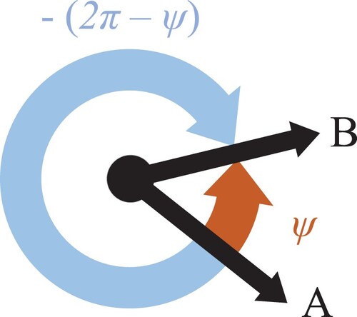
Note that we use ψ to denote an angle of rotation, Φ to denote a specific orientation (e.g. orientation of an edge or a desired end orientation), and θ to denote a minimum angle of rotation that needs to be made by an AGV.

A minimum absolute angle of rotation $\left|\theta \right|$ is defined as follows. An angle of rotation can be measured either in clockwise or counterclockwise direction. We define the counterclockwise direction to be positive, such that the angle of rotation from orientation A to orientation B for the example situation in Figure 1 is equal to ψ when turning in counterclockwise direction and equal to $\psi -2\pi$ when turning in clockwise direction.

Figure 1. Angles of rotation from orientation A to orientation B.

Vertex with two orientations, denoted by A and B. The angle of rotation from A to B in counterclockwise direction is denoted by . The angle of rotation from A to B in clockwise direction is denoted by .

The minimum absolute angle of rotation $\left|\theta \right|$ that needs to be made (either clockwise or counterclockwise) is equal to (7) $\left|\theta \right|=min\left(\right|\psi |,|\psi -2\pi \left|\right).$(7) The minimum angle of rotation θ is in counterclockwise direction if $\left|\theta \right|=\left|\psi \right|$: then $\theta =\psi =\left|\theta \right|$. The minimum angle of rotation θ is in clockwise direction if $\left|\theta \right|=|\psi -2\pi |$, then $\theta =\psi -2\pi =-\left|\theta \right|$.

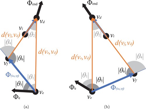
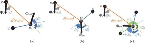
As mentioned before, the estimate $\left|{\theta }_{min}\right(v_e,v_d\left)\right|$ is a lower bound for the angles of rotation needed to move from (specified orientation ${\mathrm{\Phi }}_e$ at) vertex $v_e$ to (desired end orientation ${\mathrm{\Phi }}_{\mathrm{e}\mathrm{n}\mathrm{d}}$ at) destination vertex $v_d$. Figure 2 shows three example situations, where vertex $v_e$ (with specified orientation ${\mathrm{\Phi }}_e$ of the AGV) and destination vertex $v_d$ (with the desired end orientation ${\mathrm{\Phi }}_{\mathrm{e}\mathrm{n}\mathrm{d}}$ of the AGV) are shown as circles. The Euclidean vector (i.e. shortest possible connection regardless of the graph) directed from vertex $v_e$ to destination vertex $v_d$ is shown as the arrow connecting those vertices. Three minimum angles of rotation are shown in this figure as ${\theta }_1$, ${\theta }_2$, and ${\theta }_3$.

Figure 2. Graphic representation of the minimum absolute angles of rotation $\left|{\theta }_1\right|$, $\left|{\theta }_2\right|$, and $\left|{\theta }_3\right|$ for vertex $v_e$ with specified orientation ${\mathrm{\Phi }}_e$ and destination vertex $v_d$ with end orientation ${\mathrm{\Phi }}_{\mathrm{e}\mathrm{n}\mathrm{d}}$. (a) One incoming edge at $v_d$. The minimum angles of rotation at $v_d$ are equal to $\left|{\theta }_2\right|$ and $\left|{\theta }_3\right|$. (b) One incoming edge at $v_d$. The minimum angles of rotation at $v_d$ are equal to $-\left|{\theta }_2\right|$ and $\left|{\theta }_3\right|$, and (c) two incoming edges a and b at $v_d$.

Read the detailed description of this figure

(a) Vertices , (with, respectively, orientations and ), and are drawn in such a way that the minimum angle of rotation from to Euclidean vector is in counterclockwise direction and equal to , the minimum angle of rotation from to the edge is in counterclockwise direction and equal to , and the minimum angle of rotation from the edge to is in counterclockwise direction and equal to . (b) Vertices (with, respectively, orientations and ), and are drawn in such a way that the minimum angle of rotation from to Euclidean vector is in counterclockwise direction and equal to , the minimum angle of rotation from to the edge is in clockwise direction and equal to , and the minimum angle of rotation from the edge to is in counterclockwise direction and equal to . (c) Vertices (with, respectively, orientations and ), and two predecessor vertices of (i.e. the start vertices of edges and ) are drawn in such a way that the minimum angle of rotation from to Euclidean vector is in counterclockwise direction and equal to , the minimum angles of rotation from to the edges and are, respectively, in clockwise and counterclockwise direction and equal to, respectively, and , and the minimum angles of rotation from the edges and to are, respectively, in clockwise and counterclockwise direction and equal to, respectively, and .

The minimum angle of rotation ${\theta }_1$ represents the rotation from orientation ${\mathrm{\Phi }}_e$ at vertex $v_e$ to the Euclidean vector $d(v_e,v_d)$ directed from vertex $v_e$ to destination vertex $v_d$ with (8) $\left|{\theta }_1\right|=\left|{\theta }_{{\mathrm{\Phi }}_e\to {\mathrm{\Phi }}_{d(v_e,v_d)}}\right|.$(8) The minimum angles of rotation ${\theta }_2$ and ${\theta }_3$ are dependent on the incoming edge(s) to the destination vertex $v_d$. Those minimum angles of rotation represent, respectively, the rotation from Euclidean vector $d(v_e,v_d)$ to the incoming edge at the destination vertex $v_d$, and the rotation from that incoming edge to the desired end orientation ${\mathrm{\Phi }}_{\mathrm{e}\mathrm{n}\mathrm{d}}$. As shown in Figure 2(c), different incoming edges $(v_i,v_d)\in E$ can lead to different values for ${\theta }_2$ and ${\theta }_3$: (9) $\begin{array}{rl}|{\theta }_2{|}_{(v_i,v_d)}& =\left|{\theta }_{{\mathrm{\Phi }}_{d(v_e,v_d)}\to {\mathrm{\Phi }}_{(v_i,v_d)}}\right|,\end{array}$(9) (10) $\begin{array}{rl}|{\theta }_3{|}_{(v_i,v_d)}& =\left|{\theta }_{{\mathrm{\Phi }}_{(v_i,v_d)}\to {\mathrm{\Phi }}_{\mathrm{e}\mathrm{n}\mathrm{d}}}\right|.\end{array}$(10) In these equations, ${\mathrm{\Phi }}_{(v_i,v_d)}$ represents the orientation of edge $(v_i,v_d)\in E$.

The lower bound estimate $\left|{\theta }_{min}\right(v_e,v_d\left)\right|$ might be chosen equal to $\left|{\theta }_1\right|$ only but is sharpened by also using $\left|{\theta }_2\right|$ and $\left|{\theta }_3\right|$. It is equal to (11) $\left|{\theta }_{min}\right(v_e,v_d\left)\right|=\left|{\theta }_1\right|+\underset{(v_i,v_d)\in E}{min}(|{\theta }_2{|}_{(v_i,v_d)}+|{\theta }_3{|}_{(v_i,v_d)}).$(11) The minimum sum of $|{\theta }_2{|}_{(v_i,v_d)}$ and $|{\theta }_3{|}_{(v_i,v_d)}$ over the incoming edges $(v_i,v_d)\in E$ at the destination vertex $v_d$ is used to compute the lower bound estimate $\left|{\theta }_{min}\right(v_e,v_d\left)\right|$. If the desired end orientation ${\mathrm{\Phi }}_{\mathrm{e}\mathrm{n}\mathrm{d}}$ is unspecified, then the minimum angle of rotation ${\theta }_3$ is set to zero. Note that $\left|{\theta }_{min}\right(v_d,v_d\left)\right|$ is equal to zero.

Figure 2(a) shows an example situation for one incoming edge at the destination vertex $v_d$. In this case, the minimum angles of rotation are equal to ${\theta }_1=\left|{\theta }_1\right|$, ${\theta }_2=\left|{\theta }_2\right|$, and ${\theta }_3=\left|{\theta }_3\right|$, since they are measured in counterclockwise direction. The lower bound estimate $\left|{\theta }_{min}\right(v_e,v_d\left)\right|$ equals $\left|{\theta }_1\right|+\left|{\theta }_2\right|+\left|{\theta }_3\right|$ (see Equation (11(11) $\left|{\theta }_{min}\right(v_e,v_d\left)\right|=\left|{\theta }_1\right|+\underset{(v_i,v_d)\in E}{min}(|{\theta }_2{|}_{(v_i,v_d)}+|{\theta }_3{|}_{(v_i,v_d)}).$(11) )).

Figure 2(b) shows minimum angles of rotation ${\theta }_1$, ${\theta }_2$, and ${\theta }_3$ for a different desired end orientation ${\mathrm{\Phi }}_{\mathrm{e}\mathrm{n}\mathrm{d}}$ at the destination vertex $v_d$. In this case, the minimum angles of rotation at the destination vertex $v_d$ are equal to ${\theta }_2=-\left|{\theta }_2\right|$ and ${\theta }_3=\left|{\theta }_3\right|$, since they are measured in, respectively, clockwise and counterclockwise directions. Also for the situation shown in Figure 2(b), the lower bound estimate $\left|{\theta }_{min}\right(v_e,v_d\left)\right|$ equals $\left|{\theta }_1\right|+\left|{\theta }_2\right|+\left|{\theta }_3\right|$ (see Equation (11(11) $\left|{\theta }_{min}\right(v_e,v_d\left)\right|=\left|{\theta }_1\right|+\underset{(v_i,v_d)\in E}{min}(|{\theta }_2{|}_{(v_i,v_d)}+|{\theta }_3{|}_{(v_i,v_d)}).$(11) )).

Figure 2(c) shows an example situation with two incoming edges at the destination vertex $v_d$. The minimum angles of rotation $-|{\theta }_2{|}_a$ and $-|{\theta }_3{|}_a$ are related to the incoming edge a. The minimum angles of rotation $|{\theta }_2{|}_b$ and $|{\theta }_3{|}_b$ are related to the incoming edge b. The lower bound estimate $\left|{\theta }_{min}\right(v_e,v_d\left)\right|$ equals $\left|{\theta }_1\right|+\underset{a,b}{min}\left(\right|{\theta }_2{|}_a+|{\theta }_3{|}_a,|{\theta }_2{|}_b+\left|{\theta }_3{|}_b\right)$ (see Equation (11(11) $\left|{\theta }_{min}\right(v_e,v_d\left)\right|=\left|{\theta }_1\right|+\underset{(v_i,v_d)\in E}{min}(|{\theta }_2{|}_{(v_i,v_d)}+|{\theta }_3{|}_{(v_i,v_d)}).$(11) )).

As mentioned in Section 2, the A${}^{\ast }$ algorithm is admissible (i.e. is guaranteed to find the optimal (lowest-cost) path), if the heuristic $h(v_e,v_d)$ provides a lower bound estimate of the actual minimum costs $h^{\ast }(v_e,v_d)$ to move from vertex $v_e$ to destination vertex $v_d$. To prove that with our heuristic, the A${}^{\ast }$ algorithm finds the optimal path, we have to prove that the minimum absolute angle of rotation $\left|{\theta }_{min}\right(v_e,v_d\left)\right|$ is a lower bound estimate of the actual minimum absolute angle of rotation the AGV needs to make, to move from (specified orientation ${\mathrm{\Phi }}_e$ at) vertex $v_e$ to (desired end orientation ${\mathrm{\Phi }}_{\mathrm{e}\mathrm{n}\mathrm{d}}$ at) destination vertex $v_d$. The proof is provided in Appendix 3.

5. Comparative study

To validate the efficiency of our heuristic, we executed a comparative study. We determined the number of iterations needed by the A${}^{\ast }$ algorithm to find the lowest-cost path from each vertex to each other vertex in the layout, for different heuristics, for different types of grid layouts. The grid layouts studied have sizes of approximately $10\times 10$, $20\times 20$, $30\times 30$, and $40\times 40$ elements, with either rectangular, hexagonal, or arbitrary-shaped grid elements. Furthermore, we verified the effect of changing the values of some input parameters that affect the mutual differences between the evaluated heuristics.

In this section, we first provide the cost function used in our study in Section 5.1, which is the same for all heuristics included in the comparison. Then we describe the other heuristics included in our comparative study in Section 5.2 and the layouts used in Section 5.3. We introduce a metric that is used for comparison of the results in Section 5.4, and finally provide the results and a discussion of these results in Section 5.5.

5.1. Cost function lowest-cost path

To fairly compare the performance of our heuristic to other heuristics found in the literature, it is important that the A${}^{\ast }$ algorithm finds the same optimal (i.e. lowest-cost) path for all heuristics included in the comparison. The goal of the algorithm, for every heuristic, is to find the path minimising the cost function given in Equation (3(3) $C\left(P_{v^{\prime },v^{″}}\right)=\sum _{(v_i,v_j)\in E\left(P_{v^{\prime },v^{″}}\right)}{c}_{v_i{v}_j}+p_{\mathrm{t}\mathrm{u}\mathrm{r}\mathrm{n}}\sum _{v_i\in V\left(P_{v^{\prime },v^{″}}\right)}\left|{\theta }_{v_i}\right|.$(3) ) with $v^{\prime }=v_s$ and $v^{″}=v_d$. In the study, the weight of each edge $(v_i,v_j)$ is equal to (12) $c_{v_i{v}_j}=\frac{l_{v_i{v}_j}}{s_{max}}.$(12) In this equation, $l_{v_i{v}_j}$ is the distance from vertex $v_i$ to vertex $v_j$, and $s_{max}$ is the maximum AGV (translation) speed. The turning costs per radian are equal to (13) $p_{\mathrm{t}\mathrm{u}\mathrm{r}\mathrm{n}}=\frac{1}{{\omega }_{max}}.$(13) In this equation, ${\omega }_{max}$ is the maximum rotation speed of the AGV.

5.2. Other heuristics

The control strategies of Bae and Chung (2018), Bae and Chung (2019), Cui et al. (2018), and Lian and Xie (2019) show resemblance with our control strategy (see Table 1); therefore the performance of these strategies (in a modified version to allow for a fair comparison) are compared to the performance of our strategy. Bae and Chung (2018), Bae and Chung (2019), and Lian and Xie (2019) do not incorporate turning in the heuristic; the heuristic only consists of a term related to translation, described in Equation (5(5) $h_{\mathrm{t}\mathrm{r}\mathrm{a}\mathrm{n}\mathrm{s}}(v_e,v_d)=\frac{\left|d\right(v_e,v_d\left)\right|}{s_{max}}.$(5) ). For simplicity, we will only refer to Bae and Chung (2018). The control strategy is suitable for orthogonal grids only. However, by using rotation-dependent turning costs instead of constant turning costs (the costs for turning over $\pi /2$ radians) in the computations for $f(v_s,v_e,v_d)$ and $g(v_s,v_e)$, the control strategy can be applied to non-orthogonal grids as well.

Also the control strategy described by Cui et al. (2018) shows resemblance with our control strategy, assuming that decelerations before and accelerations after turning are infinitely large. The heuristic consists of a component related to translation and a component related to rotation, see Equation (4(4) $h(v_e,v_d)=h_{\mathrm{t}\mathrm{r}\mathrm{a}\mathrm{n}\mathrm{s}}(v_e,v_d)+h_{\mathrm{r}\mathrm{o}\mathrm{t}}(v_e,v_d).$(4) ). The component related to translation is equal to (14) $h_{\mathrm{t}\mathrm{r}\mathrm{a}\mathrm{n}\mathrm{s}}(v_e,v_d)=\frac{|x_{v_e}-x_{v_d}|+|y_{v_e}-y_{v_d}|}{s_{max}}.$(14) In this equation, $|x_{v_e}-x_{v_d}|$ is the absolute difference in x-coordinates between vertex $v_e$ and destination vertex $v_d$, and $|y_{v_e}-y_{v_d}|$ is the absolute difference in y-coordinates between vertex $v_e$ and destination vertex $v_d$. The control strategy adds constant turning costs (the costs for turning over $\pi /2$ radians) to the heuristic if both the x- and y-coordinates of the vertex $v_e$ differ from, respectively, the x- and y-coordinates of the destination vertex $v_d$. The control strategy is only suitable for orthogonal and axis-aligned grids. Changing the control strategy such that it becomes suitable for other grids as well requires major changes. The component in the heuristic related to translation should be changed to the term described in Equation (5(5) $h_{\mathrm{t}\mathrm{r}\mathrm{a}\mathrm{n}\mathrm{s}}(v_e,v_d)=\frac{\left|d\right(v_e,v_d\left)\right|}{s_{max}}.$(5) ). Furthermore, the component in the heuristic related to rotation should be removed, and rotation-dependent turning costs should be used instead of constant turning costs for the computations for $f(v_s,v_e,v_d)$ and $g(v_s,v_e)$. The control strategy then becomes similar to the control strategy developed by Bae and Chung (2018). The control strategy developed by Cui et al. (2018) will therefore only be used in the comparative study for rectangular grids.

The Manhattan distance (i.e. $|x_{v_e}-x_{v_d}|+|y_{v_e}-y_{v_d}|$) is equal to or bigger than the Euclidean distance (the triangle inequality), i.e. (15) $|x_{v_e}-x_{v_d}|+|y_{v_e}-y_{v_d}|\ge \left|d\right(v_e,v_d\left)\right|.$(15) Therefore, using the Manhattan distance in the component related to translation $h_{\mathrm{t}\mathrm{r}\mathrm{a}\mathrm{n}\mathrm{s}}(v_e,v_d)$ results in a higher cost estimate compared to using the Euclidean distance. As explained in Section 2, the closer the value of $h(v_e,v_d)$ is to the actual minimum costs $h^{\ast }(v_e,v_d)$, the lower the number of iterations needed to find the lowest-cost path. Using the Manhattan distance in the heuristic will therefore cause less (or an equal number of) iterations to be needed to find the lowest-cost path, compared to using the Euclidean distance.

The added value of our heuristic is the component related to rotation; using the Euclidean distance in the component related to translation has been done before, and the effect of using the Euclidean distance instead of the Manhattan distance has been studied before by, for example, Kusuma, Riyanto, and Machbub (2019) and MacGregor and Leung (2009). Therefore, to fairly compare the performance of the component related to rotation in our heuristic to components related to rotation in other heuristics, a modified version of the control strategy described by Cui et al. (2018) is used in the comparative study, where the component related to translation in the heuristic is as in Equation (5(5) $h_{\mathrm{t}\mathrm{r}\mathrm{a}\mathrm{n}\mathrm{s}}(v_e,v_d)=\frac{\left|d\right(v_e,v_d\left)\right|}{s_{max}}.$(5) ).

The control strategies developed by Cui et al. (2018) and Bae and Chung (2018) are not able to take into account a specified desired end orientation ${\mathrm{\Phi }}_{\mathrm{e}\mathrm{n}\mathrm{d}}$. For a fair comparison, it is necessary that all control strategies studied find the same lowest-cost path. Therefore, the comparative study is executed without specifying desired end orientation ${\mathrm{\Phi }}_{\mathrm{e}\mathrm{n}\mathrm{d}}$.

Our control strategy, as well as the modified control strategy of Cui et al. (2018), always needs less or an equal number of iterations to find the lowest-cost path, compared to the control strategy of Bae and Chung (2018). This can be explained as follows: a non-negative term is added to the heuristic of Bae and Chung (2018) in order to get our heuristic, or the modified heuristic of Cui et al. (2018). If a positive term is added, the value for the heuristic estimate increases (i.e. $h(v_e,v_d)$ gets closer to $h^{\ast }(v_e,v_d)$), resulting in a (possible) decrease in the number of iterations needed to find the lowest-cost path, as explained in Section 2. Addition of a zero term results in the same number of iterations to be needed for our heuristic, or the modified heuristic of Cui et al. (2018), compared to the heuristic of Bae and Chung (2018).

5.3. Layouts for comparative study

The layouts for the comparative study are constructed as follows:

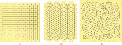
• Rectangular layouts: Square grid elements are placed in $10\times 10$, $20\times 20$, $30\times 30$, and $40\times 40$ arrangements. Horizontal and vertical driving directions are alternated over the rows and columns in such a way that strongly connected graphs (i.e. directed graphs with a path from each vertex to every other vertex) are obtained, see Figure 3(a), with vertices at the centre of each reachable grid element. Our layouts show resemblance with parcel sorting grids with alternating unidirectional lanes.

• Hexagonal layouts: Hexagonal grid elements are placed in arrangements with similar size as the rectangular layouts. However, to ensure that alternating driving directions in all three hexagonal directions (i.e. vertical and two diagonal directions) always yield a strongly connected graph, the number of columns is odd (i.e. decreased by one), and odd columns have one grid element less than even columns, see Figure 3(b).

• Arbitrary layouts: In a square enclosed space with similar dimensions as the rectangular layout, vertices are placed randomly and one by one, under the constraint that they are placed at least d metres apart (with d equal to the size of a grid element in a rectangular layout), and d/2 metre from the border of the space. The vertex generator tries to fit in as many vertices as possible, but once placed the position of a vertex is not changed anymore. A constrained Voronoi diagram is constructed to visualise the grid elements, see Figure 3(c). The unidirectional graph between the grid elements is constructed arbitrarily, nevertheless ensuring that the graph is strongly connected.

Figure 3. Layout shapes used in the comparative study. (a) Rectangular layout. (b) Hexagonal layout. (c) Arbitrary layout.

Read the detailed description of this figure

(a) Grid layout consisting of square grid elements. The centres of the grid elements are connected to neighbouring grid elements by alternating unidirectional path segments, directed from left to right at the top, and from bottom to top at the left. (b) Grid layout consisting of 9 columns of alternately 9 and 10 hexagonal grid elements. The centres of the grid elements are connected to neighbouring grid elements by alternating unidirectional path segments, directed from top to bottom at the left, from top left to bottom right, and from bottom left to top right. (c) Grid layout consisting of 71 grid elements with an arbitrary convex shape. The centres of the grid elements are connected to neighbouring grid elements by unidirectional path segments, such that the graph is fully connected.

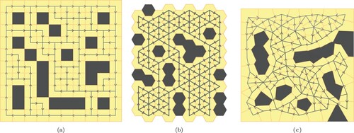
For all layout shapes and sizes, multiple instances are generated (see also Section 5.4) in which 20% of the grid elements are blocked. Figure 4 shows three example layouts with 20% of the grid elements blocked. The blocked grid elements can be regarded as obstacles where AGVs cannot drive. The grid elements that are blocked are chosen randomly, one by one, in a greedy manner: a random grid element is selected and blocked if the resulting graph remains strongly connected, otherwise the grid element is skipped. This process continues until 20% of all grid elements have been blocked or all grid elements have been evaluated.

Figure 4. Example layouts with randomly 20% of the grid elements blocked. (a) Rectangular layout. (b) Hexagonal layout. (c) Arbitrary layout.

Read the detailed description of this figure

(a) Grid layout consisting of square grid elements. The centres of the grid elements are connected to neighbouring grid elements by alternating unidirectional path segments, directed from left to right at the top, and from bottom to top at the left. Twenty grid elements in the layout are blocked; these are not connected to neighbouring grid elements. (b) Grid layout consisting of 9 columns of alternately 9 and 10 hexagonal grid elements. The centres of the grid elements are connected to neighbouring grid elements by alternating unidirectional path segments, directed from top to bottom at the left, from top left to bottom right, and from bottom left to top right. Seventeen grid elements in the layout are blocked; these are not connected to neighbouring grid elements. (c) Grid layout consisting of 71 grid elements with an arbitrary convex shape. The centres of the grid elements are connected to neighbouring grid elements by unidirectional path segments, such that the graph is fully connected. Fourteen grid elements in the layout are blocked; these are not connected to neighbouring grid elements.

5.4. Metric

For each grid layout considered, the number of iterations needed to travel from one to another vertex in the grid is determined for all possible source-destination combinations, for each heuristic. Results are generated for 0% and 20% of the grid elements blocked. For 20% of the grid elements blocked, 40 random combinations of blocked grid elements are generated in order to establish the 95% confidence interval of the mean number of iterations needed. Furthermore, for arbitrary layouts for 0% of the grid elements blocked, also 40 random arbitrary layouts are created.

We have chosen to study the difference in the number of iterations between the different heuristics and to not focus on computation time, since the measured computation time depends on the implementation of the heuristics and the computer used, while the number of iterations is independent of these variables. The number of iterations is also used in other literature as a measure for the efficiency of the A${}^{\ast }$ algorithm (e.g. in Mathew 2015; Song and Yuan 2019; Whangbo 2007; Yao et al. 2010).

The number of iterations needed to find the lowest-cost path using the A${}^{\ast }$ algorithm is the number of vertices being expanded during execution of the algorithm (Róka 2018). At least all vertices in the lowest-cost path from the source vertex $v_s$ to the predecessor vertex of the destination vertex $v_d$ need to be expanded. Therefore, the number of iterations $n\left(P_{v_s,v_d}\right)$ is at least equal to the number of grid elements (i.e. vertices) in the lowest-cost path $\left|V\right(P_{v_s,v_d}\left)\right|$ minus one (since the destination vertex $v_d$ does not have to be expanded), i.e.  (16) $\frac{n\left(P_{v_s,v_d}\right)}{\left|V\right(P_{v_s,v_d}\left)\right|-1}\ge 1.$(16) Ideally, the number of iterations is as low as possible and thus equal to the number of grid elements in the lowest-cost path (i.e. path elements) minus one.

Figure 5 shows the sample mean and 95$\mathrm{\%}$ confidence interval of $n\left(P_{v_s,v_d}\right)/\left(\right|V\left(P_{v_s,v_d}\right)|-1)$ for different path lengths, for a $30\times 30$ grid with rectangular elements, for $0\mathrm{\%}$ of the grid elements blocked. Only the path lengths with at least 40 samples are shown to allow for the computation of confidence intervals. The parameter values used for the computations are provided in Table 2. As shown in Figure 5, for longer paths, the average number of iterations needed to find one element of the lowest-cost path is relatively large; the longer the path $P_{v_s,v_d}$, the larger $n\left(P_{v_s,v_d}\right)/\left(\right|V\left(P_{v_s,v_d}\right)|-1)$. Due to an upper bound on the number of iterations (since the number of vertices in the graph is finite and the heuristic is monotone), an S-curve is visible in the figure. Since the number of grid elements in the path is also larger for longer paths, efficiency gains for longer paths are thought to have a significant influence on the performance of a heuristic. To properly take this into account, the following performance metric is defined to measure the performance of a heuristic for a specific layout: (17) $\frac{\sum _{v_s,v_d\in V}n\left(P_{v_s,v_d}\right)}{\sum _{v_s,v_d\in V}\left(\right|V\left(P_{v_s,v_d}\right)|-1)}.$(17) This metric can be interpreted as the weighted average number of iterations needed to find one grid element of the lowest-cost path (i.e. path element). It is at least equal to one; the better the heuristic, the closer the value is to one.

Figure 5. Average number of iterations needed to find one grid element of the lowest-cost path (i.e. path element), for different path lengths, for a $30\times 30$ rectangular grid with $0\mathrm{\%}$ of the grid elements blocked.

2D plot showing the sample mean and 95% confidence interval for the number of iterations per path element, for different path lengths, for the control strategies of Bae and Chung (), modified Cui et al. (), and Heuristic This Paper. An S-curve in the results is visible for all control strategies, starting from bottom left to top right.

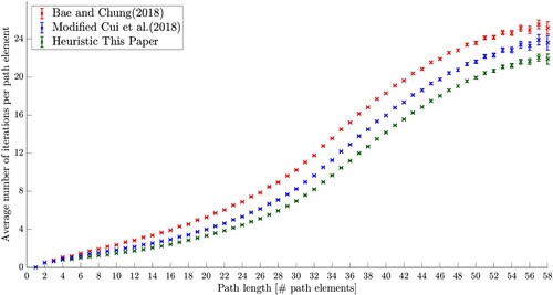
Table 2. Parameter values used for the computations.

Parameter	Value
Maximum (translation) speed, $s_{max}$ (m/s)	2
Size grid element (m)	2
Maximum rotation speed, ${\omega }_{max}$ (rad/s)	$\pi /2$
Start orientation ${\mathrm{\Phi }}_{\mathrm{s}\mathrm{t}\mathrm{a}\mathrm{r}\mathrm{t}}$ of AGV at source vertex $v_s$ (rad)	0

5.5. Results and discussion

The resulting performance metrics of the computations executed for the control strategy with our heuristic, the modified heuristic of Cui et al. (2018), and the heuristic defined by Bae and Chung (2018) equal to the heuristics defined by Bae and Chung (2019) and Lian and Xie (2019) and are visible in Figure 6. The figure shows the sample mean and 95$\mathrm{\%}$ confidence interval of the metric for different grid sizes. The parameter values used for the computations are provided in Table 2. Results are shown for grids with, respectively, rectangular, hexagonal, and arbitrary-shaped grid elements, for approximately $10\times 10$, $20\times 20$, $30\times 30$, and $40\times 40$ elements, for, respectively, $0\mathrm{\%}$ and $20\mathrm{\%}$ of the grid elements blocked.

Figure 6. Computed metrics for grids with different element shapes, for different percentages of grid elements blocked, and for different grid sizes. (a) Grid with rectangular elements, with $0\mathrm{\%}$ of the grid elements blocked. (b) Grid with rectangular elements, with $20\mathrm{\%}$ of the grid elements blocked. (c) Grid with hexagonal elements, with $0\mathrm{\%}$ of the grid elements blocked. (d) Grid with hexagonal elements, with $20\mathrm{\%}$ of the grid elements blocked. (e) Grid with arbitrary-shaped elements, with $0\mathrm{\%}$ of the grid elements blocked. (f) Grid with arbitrary-shaped elements, with $20\mathrm{\%}$ of the grid elements blocked.

Read the detailed description of this figure

(a) 2D plot showing the sample mean and 95% confidence interval for the metric (i.e. the weighted average number of iterations per path element), for different grid sizes, and for (in descending order of the sample mean for each grid size) control strategies of Bae and Chung (), modified Cui et al. (), and Heuristic This Paper. There is no overlap in confidence intervals between different control strategies. (b) 2D plot showing the sample mean and 95% confidence interval for the metric (i.e. the weighted average number of iterations per path element), for different grid sizes, and for (in descending order of the sample mean for each grid size) control strategies of Bae and Chung (), modified Cui et al. (), and Heuristic This Paper. There is no overlap in confidence intervals between different control strategies. (c) 2D plot showing the sample mean and 95% confidence interval for the metric (i.e. the weighted average number of iterations per path element), for different grid sizes, and for (in descending order of the sample mean for each grid size) control strategies of Bae and Chung () and Heuristic This Paper. There is no overlap in confidence intervals between different control strategies. (d) 2D plot showing the sample mean and 95% confidence interval for the metric (i.e. the weighted average number of iterations per path element), for different grid sizes, and for (in descending order of the sample mean for each grid size) control strategies of Bae and Chung () and Heuristic This Paper. There is no overlap in confidence intervals between different control strategies. (e) 2D plot showing the sample mean and 95% confidence interval for the metric (i.e. the weighted average number of iterations per path element), for different grid sizes, and for (in descending order of the sample mean for each grid size) control strategies of Bae and Chung () and Heuristic This Paper. There is no overlap in confidence intervals between different control strategies. (f) 2D plot showing the sample mean and 95% confidence interval for the metric (i.e. the weighted average number of iterations per path element), for different grid sizes, and for (in descending order of the sample mean for each grid size) control strategies of Bae and Chung () and Heuristic This Paper. There is no overlap in confidence intervals between different control strategies.

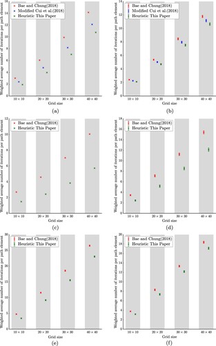
Figure 6 shows that the mutual differences between the evaluated heuristics remain approximately constant for different grid sizes. Our control strategy needs on average the lowest number of iterations to find the lowest-cost path, followed by the modified control strategy of Cui et al. (2018) for rectangular grids, and, as expected, the control strategy of Bae and Chung (2018).

For rectangular grids, our control strategy does not always outperform the modified control strategy of Cui et al. (2018); for specific combinations of source vertex $v_s$ and destination vertex $v_d$ (for example, when the Euclidean vector $d(v_s,v_d)$ directed from source vertex $v_s$ to destination vertex $v_d$ is almost (but not exactly) parallel to an axis, with incoming edges at source vertex $v_s$ and destination vertex $v_d$ aligned with the axis), the number of iterations needed by the modified control strategy of Cui et al. (2018) may be less than the number of iterations needed by our control strategy. However, on average our control strategy outperforms the modified control strategy of Cui et al. (2018). Furthermore, the modified control strategy of Cui et al. (2018) cannot be used for grids with hexagonal or arbitrary-shaped elements.

The mutual differences between control strategies are influenced by the parameter values used for the computations: the values selected for maximum rotation speed ${\omega }_{max}$ and maximum (translation) speed $s_{max}$ may influence the ratio between the values of the components in the heuristic related to rotation and translation. For ${\omega }_{max}\to \mathrm{\infty }$ or $s_{max}\to 0$, the component in the heuristic related to translation will dominate the component related to rotation; the performance of all control strategies will be similar. For ${\omega }_{max}\to 0$ or $s_{max}\to \mathrm{\infty }$, the component in the heuristic related to rotation will dominate the component related to translation, increasing the mutual differences between control strategies. This behaviour is also visible in the computations executed for a $30\times 30$ rectangular grid with $0\mathrm{\%}$ of the grid elements blocked, for different parameter combinations: for ${\omega }_{max}\in \{1/4\pi ,1/2\pi ,3/4\pi ,\pi \}$ rad/s, and for $s_{max}\in \{0.5,2,3.5,5\}$ m/s. The results are visible in Figure 7.

Figure 7. Average number of iterations needed to find one element of the lowest-cost path for different combinations of maximum (translation) speed and maximum rotation speed, for a $30\times 30$ rectangular grid with $0\mathrm{\%}$ of the grid elements blocked.

3D plot showing the metric (i.e. the weighted average number of iterations per path element) for different speeds and rotation speeds and for (in descending order of the sample mean for each combination of speeds) control strategies of Bae and Chung (), modified Cui et al. (), and Heuristic This Paper. There is no overlap in 3D plots between different control strategies.

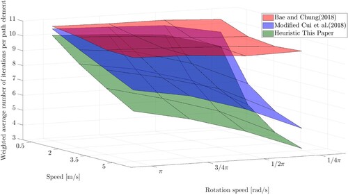
The figure shows that our heuristic outperforms the other heuristics for all parameter values; the differences become larger for smaller maximum rotation speeds and larger maximum (translation) speeds.

6. Conclusion

In this paper, we have provided a literature overview of existing work on path planning using the A${}^{\ast }$ algorithm on a geometric graph with turning costs. In general, in the current literature either turning costs are not taken into account in the heuristic or the heuristic can only be used for specific graph structures. We have not found any proofs of heuristics' admissibility.

We developed a monotone and admissible A${}^{\ast }$ heuristic incorporating turning costs that can be used for any geometric graph structure. We validated that our heuristic decreases the number of iterations needed to find the lowest-cost path, compared to other heuristics found in the literature. A decrease of up to $68\mathrm{\%}$ for the weighted average number of iterations needed to find one vertex in the lowest-cost path was achieved, depending on the selected input parameters. Using information about the graph structure in the heuristic can further decrease the number of iterations needed. For example, for rectangular grids, the Manhattan distance can be used instead of the Euclidean distance. For some rectangular grids, it may be beneficial to take the maximum of our heuristic and the heuristic developed by Cui et al. (2018). However, the heuristic can then no longer be used for any graph structure.

Furthermore, for any graph structure, the directions of outgoing edges at the current vertex (besides the currently used directions of incoming edges at the destination vertex) can be included to further improve the heuristic.

Although the component related to rotation in our heuristic decreases the number of iterations needed to find the lowest-cost path in the A${}^{\ast }$ algorithm, we have increased the number of operations needed to compute the heuristic. Pre-computation of heuristic values is possible to decrease the number of extra operations needed. Depending on the selected input parameter values and weights in the graph, the extra complexity in the heuristic may not be beneficial (e.g. if the turning costs are zero). A recommendation for improvement is to study if our heuristic of the A${}^{\ast }$ algorithm could be made self-configuring based on the graph and parameters such as turning costs.

Acknowledgments

We would like to thank Erjen Lefeber for his help in proving the admissibility of the component related to rotation in our heuristic.

Disclosure statement

No potential conflict of interest was reported by the authors.

Data availability statement

The data that support the findings of this study are available from the corresponding author upon reasonable request.

Additional information

Notes on contributors

Karlijn Fransen

Karlijn Fransen is a Ph.D. candidate at the Control Systems Technology Group, Department of Mechanical Engineering, Eindhoven University of Technology, The Netherlands, as well as System Architect at Vanderlande, supplier of logistic process automation solutions. She received her M.S. degree in both Mechanical Engineering and Industrial and Applied Mathematics, and her B.S. degree in Mechanical Engineering from Eindhoven University of Technology, The Netherlands. Her research interests include algorithm development for system-level controls of AGV systems.

Joost van Eekelen

Joost van Eekelen is currently an Assistant Professor with the Eindhoven University of Technology (The Netherlands), in the Control Systems Technology Group of the Mechanical Engineering Department, as well as a System Architect with Vanderlande, supplier of automated logistic solutions. Joost received both his M.S. and Ph.D. degrees from the aforementioned university, with the Systems Engineering Group, in 2003 and 2008, respectively. His research interests include modelling, control, analysis, and optimisation of AGVs, flexible manufacturing system topology synthesis, and model-based systems engineering.

Appendices

Appendix 1.

Pseudocode A${}^{\ast }$ algorithm

In this appendix, the pseudocode of the A${}^{\ast }$ algorithm, adapted from Yao et al. (2010), is provided in Algorithm 1. This algorithm makes use of Algorithms 2 and 3. The A${}^{\ast }$ algorithm is used to find the lowest-cost path $P_{v_s,v_d}$ from source vertex $v_s$ to destination vertex $v_d$ on a graph $G=(V,E)$ with costs related to translation and rotation. We assume that vertex $v_d\in V$ is reachable from vertex $v_s\in V$. We developed a new heuristic $h(v_e,v_d)$ (see Equation (4(4) $h(v_e,v_d)=h_{\mathrm{t}\mathrm{r}\mathrm{a}\mathrm{n}\mathrm{s}}(v_e,v_d)+h_{\mathrm{r}\mathrm{o}\mathrm{t}}(v_e,v_d).$(4) )) that can be used to find the path minimising the cost function in Equation (3(3) $C\left(P_{v^{\prime },v^{″}}\right)=\sum _{(v_i,v_j)\in E\left(P_{v^{\prime },v^{″}}\right)}{c}_{v_i{v}_j}+p_{\mathrm{t}\mathrm{u}\mathrm{r}\mathrm{n}}\sum _{v_i\in V\left(P_{v^{\prime },v^{″}}\right)}\left|{\theta }_{v_i}\right|.$(3) ). The term related to our contribution is the term containing $p_{\mathrm{t}\mathrm{u}\mathrm{r}\mathrm{n}}$ in line 4 of Algorithm 3. The symbols used in the algorithms (and their meaning) are provided in Table A1.

Table B1. Symbols and their meaning in Algorithms 1–3.

Symbol	Meaning
E	Set of all edges in graph $G=(V,E)$
$v_s$	Source vertex
$v_d$	Destination vertex
$p_{\mathrm{t}\mathrm{u}\mathrm{r}\mathrm{n}}$	Turning costs per radian
c	Set of all edge weights $c_{v_i{v}_j}$ for all edges E
$s_{max}$	Maximum AGV speed
${\mathrm{\Phi }}_{\mathrm{s}\mathrm{t}\mathrm{a}\mathrm{r}\mathrm{t}}$	Start orientation
${\mathrm{\Phi }}_{\mathrm{e}\mathrm{n}\mathrm{d}}$	End orientation
$P_{v_s,v_d}$	Lowest-cost path from source vertex $v_s$ to destination vertex $v_d$
$v_x.g$	Actual costs (found so far) from source vertex $v_s$ to vertex $v_x$ (i.e. value for $g(v_s,v_x)$)
$v_x.h$	Estimated costs (found so far) from vertex $v_x$ to destination vertex $v_d$ (i.e. value for $h(v_x,v_d)$)
$v_x.f$	Lowest value for actual costs plus estimated costs found so far, from source vertex $v_s$ to destination vertex $v_d$ via vertex $v_x$ (i.e. value for $f(v_s,v_x,v_d)$)
$v_x.\mathrm{p}\mathrm{r}\mathrm{e}\mathrm{d}$	Predecessor of vertex $v_x$ in lowest-cost path (found so far)
$L_{\mathrm{o}\mathrm{p}\mathrm{e}\mathrm{n}}$	Set with all open vertices (i.e. vertices to expand)
$L_{\mathrm{c}\mathrm{l}\mathrm{o}\mathrm{s}\mathrm{e}\mathrm{d}}$	Set with all closed vertices (i.e. vertices that have been expanded)
$v_c$	Current vertex
$v_{\mathrm{s}\mathrm{u}\mathrm{c}\mathrm{c}}$	Successor vertex
$g^{\prime }$	Actual costs (found so far) from source vertex $v_s$ to vertex $v_{\mathrm{s}\mathrm{u}\mathrm{c}\mathrm{c}}$ (with current vertex $v_c$ as predecessor)
$h^{\prime }$	Estimated costs from vertex $v_{\mathrm{s}\mathrm{u}\mathrm{c}\mathrm{c}}$ (with current vertex $v_c$ as predecessor) to destination vertex $v_d$
$f^{\prime }$	Value for actual costs (found so far) plus estimated costs, from source vertex $v_s$ to destination vertex $v_d$ via vertex $v_{\mathrm{s}\mathrm{u}\mathrm{c}\mathrm{c}}$ (with current vertex $v_c$ as predecessor)
$\left|\theta \right|$	Minimum absolute angle of rotation
${\mathrm{\Phi }}_{(v_x,v_y})$	Orientation of edge $(v_x,v_y)\in E$
$\left|d\right(v_e,v_d\left)\right|$	Magnitude of the Euclidean vector $d(v_e,v_d)$ directed from vertex $v_e$ to destination vertex $v_d$

Appendix 2.

Monotonicity proof

In this appendix, we provide the proof that our heuristic is monotone.

Theorem A.1

Our heuristic $h(v_e,v_d)=\left(\left|d\right(v_e,v_d\left)\right|/s_{max}\right)+p_{\mathrm{t}\mathrm{u}\mathrm{r}\mathrm{n}}\left|{\theta }_{min}\right(v_e,v_d\left)\right|$ with $\left|{\theta }_{min}\right(v_e,v_d\left)\right|$ specified in Equation (11(11) $\left|{\theta }_{min}\right(v_e,v_d\left)\right|=\left|{\theta }_1\right|+\underset{(v_i,v_d)\in E}{min}(|{\theta }_2{|}_{(v_i,v_d)}+|{\theta }_3{|}_{(v_i,v_d)}).$(11) ) is monotone.

Proof.

A heuristic is monotone (also called consistent) if it satisfies the following (in)equality (Hart, Nilsson, and Raphael 1968): (A1) $h(v_e,v_d)\le C\left(P_{v_e,v_f}\right)+h(v_f,v_d)$(A1) for each vertex $v_e\in V$ and each edge $(v_e,v_f)\in E$. Furthermore, $h(v_d,v_d)=0$ should be true.

In our case, $h(v_d,v_d)=\left(\left|d\right(v_d,v_d\left)\right|/s_{max}\right)+p_{\mathrm{t}\mathrm{u}\mathrm{r}\mathrm{n}}\left|{\theta }_{min}\right(v_d,v_d\left)\right|$. Since $\left|d\right(v_d,v_d\left)\right|=0$ and $\left|{\theta }_{min}\right(v_d,v_d\left)\right|=0$, $h(v_d,v_d)=0$ is true. To prove that Equation (A1(A1) $h(v_e,v_d)\le C\left(P_{v_e,v_f}\right)+h(v_f,v_d)$(A1) ) is satisfied, we rewrite it using Equations (3(3) $C\left(P_{v^{\prime },v^{″}}\right)=\sum _{(v_i,v_j)\in E\left(P_{v^{\prime },v^{″}}\right)}{c}_{v_i{v}_j}+p_{\mathrm{t}\mathrm{u}\mathrm{r}\mathrm{n}}\sum _{v_i\in V\left(P_{v^{\prime },v^{″}}\right)}\left|{\theta }_{v_i}\right|.$(3) )–(6(6) $h_{\mathrm{r}\mathrm{o}\mathrm{t}}(v_e,v_d)=p_{\mathrm{t}\mathrm{u}\mathrm{r}\mathrm{n}}\left|{\theta }_{min}\right(v_e,v_d\left)\right|.$(6) ): (A2) $\begin{array}{rl}& \frac{\left|d\right(v_e,v_d\left)\right|}{s_{max}}+p_{\mathrm{t}\mathrm{u}\mathrm{r}\mathrm{n}}\left|{\theta }_{min}\right(v_e,v_d\left)\right|\\ & \le c_{v_e{v}_f}+p_{\mathrm{t}\mathrm{u}\mathrm{r}\mathrm{n}}\left(\right|{\theta }_{v_e}|+|{\theta }_{v_f}\left|\right)+\frac{\left|d\right(v_f,v_d\left)\right|}{s_{max}}\\ & +p_{\mathrm{t}\mathrm{u}\mathrm{r}\mathrm{n}}\left|{\theta }_{min}\right(v_f,v_d\left)\right|,\end{array}$(A2) with $c_{v_e{v}_f}\ge \left|d\right(v_e,v_f\left)\right|/s_{max}$ (due to assumptions stated in Section 4.1). Using the triangle inequality, we know (A3) $\frac{\left|d\right(v_e,v_d\left)\right|}{s_{max}}\le \frac{\left|d\right(v_e,v_f\left)\right|}{s_{max}}+\frac{\left|d\right(v_f,v_d\left)\right|}{s_{max}}.$(A3) Therefore, in order to prove monotonicity, it suffices to prove (A4) $p_{\mathrm{t}\mathrm{u}\mathrm{r}\mathrm{n}}\left|{\theta }_{min}\right(v_e,v_d\left)\right|\le p_{\mathrm{t}\mathrm{u}\mathrm{r}\mathrm{n}}\left(\right|{\theta }_{v_e}|+|{\theta }_{v_f}\left|\right)+p_{\mathrm{t}\mathrm{u}\mathrm{r}\mathrm{n}}\left|{\theta }_{min}\right(v_f,v_d\left)\right|$(A4) or (A5) $\left|{\theta }_{min}\right(v_e,v_d\left)\right|\le \left|{\theta }_{v_e}\right|+\left|{\theta }_{v_f}\right|+\left|{\theta }_{min}\right(v_f,v_d\left)\right|$(A5) with $\left|{\theta }_{min}\right(v_e,v_d\left)\right|$ specified in Equation (11(11) $\left|{\theta }_{min}\right(v_e,v_d\left)\right|=\left|{\theta }_1\right|+\underset{(v_i,v_d)\in E}{min}(|{\theta }_2{|}_{(v_i,v_d)}+|{\theta }_3{|}_{(v_i,v_d)}).$(11) ). The right-hand side of Equation (A5(A5) $\left|{\theta }_{min}\right(v_e,v_d\left)\right|\le \left|{\theta }_{v_e}\right|+\left|{\theta }_{v_f}\right|+\left|{\theta }_{min}\right(v_f,v_d\left)\right|$(A5) ) is as small as possible if an edge $(v_i,v_d)\in E$ exists that is oriented in parallel with $d(v_f,v_d)$, and if also ${\mathrm{\Phi }}_{\mathrm{e}\mathrm{n}\mathrm{d}}$ is located in parallel with $d(v_f,v_d)$. In that case (A6) $\left|{\theta }_{min}\right(v_f,v_d\left)\right|=\left|{\theta }_{{\mathrm{\Phi }}_{(v_e,v_f)}\to {\mathrm{\Phi }}_{d(v_f,v_d)}}\right|.$(A6) This implies it suffices to prove (A7) $\left|{\theta }_{min}\right(v_e,v_d\left)\right|\le \left|{\theta }_{v_e}\right|+\left|{\theta }_{v_f}\right|+\left|{\theta }_{{\mathrm{\Phi }}_{(v_e,v_f)}\to {\mathrm{\Phi }}_{d(v_f,v_d)}}\right|.$(A7) It is sufficient to prove that this (in)equality holds for the incoming edge $(v_i,v_d)\in E$ and for end orientation ${\mathrm{\Phi }}_{\mathrm{e}\mathrm{n}\mathrm{d}}$ located in parallel with $d(v_f,v_d)$, since either $(v_i,v_d)$ is the incoming edge to destination vertex $v_d$ that minimises the expression for $\left|{\theta }_{min}\right(v_e,v_d\left)\right|$ or it is one of other incoming edges to the destination vertex $v_d$ (that does not minimise $\left|{\theta }_{min}\right(v_e,v_d\left)\right|$) that provides a higher lower bound. So, for incoming edge $(v_i,v_d)\in E$ to destination vertex $v_d$, we have to prove (A8) $\begin{array}{rl}& \left|{\theta }_{{\mathrm{\Phi }}_e\to {\mathrm{\Phi }}_{d(v_e,v_d)}}\right|+\left|{\theta }_{{\mathrm{\Phi }}_{d(v_e,v_d)}\to {\mathrm{\Phi }}_{d(v_f,v_d)}}\right|\\ & \le \left|{\theta }_{v_e}\right|+\left|{\theta }_{v_f}\right|+\left|{\theta }_{{\mathrm{\Phi }}_{(v_e,v_f)}\to {\mathrm{\Phi }}_{d(v_f,v_d)}}\right|,\end{array}$(A8) with the specified orientation ${\mathrm{\Phi }}_e$ at vertex $v_e$ equal to ${\mathrm{\Phi }}_{\mathrm{s}\mathrm{t}\mathrm{a}\mathrm{r}\mathrm{t}}$ if $v_e=v_s$ or otherwise ${\mathrm{\Phi }}_e={\mathrm{\Phi }}_{(v_h,v_e)}$ with $v_h$ the predecessor vertex of vertex $v_e$.

First we assume $v_f\ne v_d$ such that $\left|{\theta }_{v_e}\right|+\left|{\theta }_{v_f}\right|=\left|{\theta }_{{\mathrm{\Phi }}_e\to {\mathrm{\Phi }}_{(v_e,v_f)}}\right|$ (see Section 4.1.2). Given $v_e$, $v_f$, and $v_d$, we can always construct a triangle with end points $v_e$, $v_f$, and $v_d$ (see, for example, Figure A1).

Figure A1. Minimum absolute angles of rotation $\left|{\theta }_1\right|$, $\left|{\theta }_2\right|$, $\left|{\theta }_4\right|$, $\left|{\theta }_5\right|$, and $\left|{\theta }_6\right|$. (a) $\left|{\theta }_1\right|>\left|{\theta }_5\right|$ and (b) $\left|{\theta }_1\right|<\left|{\theta }_5\right|$.

(a) Vertices (with, respectively, orientations and ), , and are drawn in such a way that the minimum angles of rotation , and are all in counterclockwise direction, and such that . (b) Vertices (with, respectively, orientations and ), , and are drawn in such a way that the minimum angles of rotation and are in counterclockwise direction, and and are in clockwise direction, and such that .

From now on, we use $\left|{\theta }_1\right|=\left|{\theta }_{{\mathrm{\Phi }}_e\to {\mathrm{\Phi }}_{d(v_e,v_d)}}\right|$, $\left|{\theta }_2\right|=\left|{\theta }_{{\mathrm{\Phi }}_{d(v_e,v_d)}\to {\mathrm{\Phi }}_{d(v_f,v_d)}}\right|$, $\left|{\theta }_4\right|=\left|{\theta }_{{\mathrm{\Phi }}_{(v_e,v_f)}\to {\mathrm{\Phi }}_{d(v_f,v_d)}}\right|$, and $\left|{\theta }_5\right|=\left|{\theta }_{{\mathrm{\Phi }}_e\to {\mathrm{\Phi }}_{(v_e,v_f)}}\right|$. Note that $\left|{\theta }_3\right|$ is not defined here to avoid confusion with the main text of this paper. The minimum angles of rotation ${\theta }_1$, ${\theta }_2$, ${\theta }_4$, and ${\theta }_5$ can either be acute, right, obtuse, or straight. Note that, by definition, none of the absolute minimum angles of rotation will be larger than π radians.

In case $\left|{\theta }_1\right|\ge \left|{\theta }_5\right|$ (see, for example, Figure A1(a)), then, irrespective of the types of angles ${\theta }_2$ and ${\theta }_4$, the following equations hold (respectively, straight angle property and triangle property): (A9) $\begin{array}{rl}\left|{\theta }_6\right|& =\pi -\left|{\theta }_4\right|,\end{array}$(A9) (A10) $\begin{array}{rl}\left|{\theta }_6\right|& =\pi -\left|{\theta }_2\right|-\left(\right|{\theta }_1|-|{\theta }_5\left|\right),\end{array}$(A10) so $\left|{\theta }_4\right|=\left|{\theta }_2\right|+\left|{\theta }_1\right|-\left|{\theta }_5\right|$ and $\left|{\theta }_1\right|+\left|{\theta }_2\right|=\left|{\theta }_4\right|+\left|{\theta }_5\right|$. We have proven Equation (A8(A8) $\begin{array}{rl}& \left|{\theta }_{{\mathrm{\Phi }}_e\to {\mathrm{\Phi }}_{d(v_e,v_d)}}\right|+\left|{\theta }_{{\mathrm{\Phi }}_{d(v_e,v_d)}\to {\mathrm{\Phi }}_{d(v_f,v_d)}}\right|\\ & \le \left|{\theta }_{v_e}\right|+\left|{\theta }_{v_f}\right|+\left|{\theta }_{{\mathrm{\Phi }}_{(v_e,v_f)}\to {\mathrm{\Phi }}_{d(v_f,v_d)}}\right|,\end{array}$(A8) ) to hold in this case.

In case $\left|{\theta }_1\right|\le \left|{\theta }_5\right|$ (see, for example, Figure A1(b)), we prove Equation (A8(A8) $\begin{array}{rl}& \left|{\theta }_{{\mathrm{\Phi }}_e\to {\mathrm{\Phi }}_{d(v_e,v_d)}}\right|+\left|{\theta }_{{\mathrm{\Phi }}_{d(v_e,v_d)}\to {\mathrm{\Phi }}_{d(v_f,v_d)}}\right|\\ & \le \left|{\theta }_{v_e}\right|+\left|{\theta }_{v_f}\right|+\left|{\theta }_{{\mathrm{\Phi }}_{(v_e,v_f)}\to {\mathrm{\Phi }}_{d(v_f,v_d)}}\right|,\end{array}$(A8) ) holds based on Euclid's exterior angle theorem, stating $\left|{\theta }_4\right|>max\left(\right|{\theta }_2|,|{\theta }_5|-|{\theta }_1\left|\right)$, so $\left|{\theta }_4\right|>\left|{\theta }_2\right|$. Since $\left|{\theta }_1\right|\le \left|{\theta }_5\right|$, $\left|{\theta }_1\right|+\left|{\theta }_2\right|\le \left|{\theta }_4\right|+\left|{\theta }_5\right|$. So we have proven our heuristic to be monotone for $v_f\ne v_d$.

For $v_f=v_d$, $h(v_f,v_d)=h(v_d,v_d)=0$, so $h(v_e,v_d)\le C\left(P_{v_e,v_d}\right)=h^{\ast }(v_e,v_d)$ should hold. Since our heuristic is admissible (see proof in Appendix 3), this (in)equality is satisfied and our heuristic is also monotone for $v_f=v_d$.

Appendix 3.

Admissibility proof

In this appendix, we provide the proof that our heuristic is admissible.

Theorem A.2

If an arbitrary continuous curve (i.e. path) is considered from vertex $v_e$ to destination vertex $v_d$, in the plane of the graph, such that vertex $v_e$ is left and destination vertex $v_d$ is entered with minimum absolute angle of rotation with respect to the Euclidean vector $d(v_e,v_d)$ (directed from vertex $v_e$ to destination vertex $v_d$) equal to, respectively, $\left|{\theta }_1\right|$ and $\left|{\theta }_2\right|$, then the minimum absolute angle of rotation made while moving along the curve is equal to $\left|{\theta }_1\right|+\left|{\theta }_2\right|$.

Proof.

Without loss of generality, the graph can be moved such that vertex $v_e$ is located in the origin of the Cartesian plane, and such that the Euclidean vector $d(v_e,v_d)$ is aligned with the x-axis. Furthermore, without loss of generality, the graph can be scaled such that destination vertex $v_d$ is located in $(1,0)$. The Euclidean vector $d(v_e,v_d)$ is then directed from $(0,0)$ to $(1,0)$.

Now assume the curve leaves the origin with minimum absolute angle of rotation with respect to the Euclidean vector $d(v_e,v_d)$ equal to $\left|{\theta }_1\right|$, and enters $(1,0)$ with minimum absolute angle of rotation with respect to the Euclidean vector $d(v_e,v_d)$ equal to $\left|{\theta }_2\right|$.

Without loss of generality, we can assume that the origin is left with a positive minimum angle of rotation in counterclockwise direction (i.e. with minimum angle of rotation equal to ${\theta }_1=\left|{\theta }_1\right|$). If this does not hold, the graph can be mirrored around the Euclidean vector $d(v_e,v_d)$.

The destination vertex $v_d$ can be entered with a positive or negative minimum angle of rotation (equal to $\left|{\theta }_2\right|$ in absolute value) in counterclockwise direction. We now prove the theorem for both cases.

When the destination vertex $v_d$ is entered with a negative minimum angle of rotation in counterclockwise direction (i.e. ${\theta }_2=-\left|{\theta }_2\right|$), then the difference between minimum angle of rotation from leaving the vertex $v_e$ to entering the destination vertex $v_d$ is equal to $\left|{\theta }_1\right|+\left|{\theta }_2\right|$. Since the curve is continuous, all values in between are assumed, so the minimum absolute angle of rotation made while moving along the curve is at least equal to $\left|{\theta }_1\right|+\left|{\theta }_2\right|$.

When the destination vertex $v_d$ is entered with a positive minimum angle of rotation in counterclockwise direction (i.e. ${\theta }_2=\left|{\theta }_2\right|$), then according to the mean value theorem of Cauchy, an orientation in parallel to the Euclidean vector $d(v_e,v_d)$ should be attained along the curve in order to move from vertex $v_e$ to destination vertex $v_d$. So, the orientation of a movement along the curve starts with $\left|{\theta }_1\right|$, then attains zero, and eventually becomes $\left|{\theta }_2\right|$. The minimum absolute angle of rotation that should therefore at least be made while moving along the curve is equal to $\left|{\theta }_1\right|$ (from $\left|{\theta }_1\right|$ to 0) plus $\left|{\theta }_2\right|$ (from 0 to $\left|{\theta }_2\right|$).

Theorem A.3

The sum of minimum absolute angles of rotation $\left|{\theta }_{min}\right(v_e,v_d\left)\right|$ as computed in Equation (11(11) $\left|{\theta }_{min}\right(v_e,v_d\left)\right|=\left|{\theta }_1\right|+\underset{(v_i,v_d)\in E}{min}(|{\theta }_2{|}_{(v_i,v_d)}+|{\theta }_3{|}_{(v_i,v_d)}).$(11) ) is a lower bound estimate of the actual minimum absolute angle of rotation the AGV needs to make, to move from (specified orientation ${\mathrm{\Phi }}_e$ at) vertex $v_e$ to (desired end orientation ${\mathrm{\Phi }}_{\mathrm{e}\mathrm{n}\mathrm{d}}$ at) destination vertex $v_d$.

Proof.

Theorem A.2 states that the minimum absolute angle of rotation the AGV needs to make, to move along an arbitrary path from vertex $v_e$ to destination vertex $v_d$, such that vertex $v_e$ is left and destination vertex $v_d$ is entered with minimum absolute angle of rotation with respect to the Euclidean vector $d(v_e,v_d)$ (directed from vertex $v_e$ to destination vertex $v_d$) equal to, respectively, $\left|{\theta }_1\right|$ and $\left|{\theta }_2\right|$, is equal to $\left|{\theta }_1\right|+\left|{\theta }_2\right|$. In order to reach the desired end orientation ${\mathrm{\Phi }}_{\mathrm{e}\mathrm{n}\mathrm{d}}$ at the destination vertex $v_d$, an extra minimum absolute angle of rotation needs to be made of at least $\left|{\theta }_3\right|$. For one incoming edge (i.e. for one possibility of entering the destination vertex $v_d$), the minimum absolute angle of rotation the AGV needs to make is therefore at least equal to $\left|{\theta }_1\right|+\left|{\theta }_2\right|+\left|{\theta }_3\right|$.

For multiple incoming edges at the destination vertex $v_d$, considering the incoming edge $(v_i,v_d)\in E$ that minimises $|{\theta }_2{|}_{(v_i,v_d)}+|{\theta }_3{|}_{(v_i,v_d)}$ ensures that Equation (11(11) $\left|{\theta }_{min}\right(v_e,v_d\left)\right|=\left|{\theta }_1\right|+\underset{(v_i,v_d)\in E}{min}(|{\theta }_2{|}_{(v_i,v_d)}+|{\theta }_3{|}_{(v_i,v_d)}).$(11) ) provides a lower bound estimate of the actual minimum absolute angle of rotation needed.

References

- Anavatti, S. G., S. L. Francis, and M. Garratt. 2016. “Path-Planning Modules for Autonomous Vehicles: Current Status and Challenges.” 2015 International Conference on Advanced Mechatronics, Intelligent Manufacture, and Industrial Automation (ICAMIMIA), Surabaya, Indonesia, October 15-17, 205–214.
- Bae, J., and W. Chung. 2018. “A Heuristic for Path Planning of Multiple Heterogeneous Automated Guided Vehicles.” International Journal of Precision Engineering and Manufacturing 19 (12): 1765–1771.
- Bae, J., and W. Chung. 2019. “Efficient Path Planning for Multiple Transportation Robots Under Various Loading Conditions.” International Journal of Advanced Robotic Systems 16 (2): 1–9.
- Ballamajalu, R., M. Li, F. Sahin, C. Hochgraf, R. Ptucha, and M. E. Kuhl. 2020, August 20-21. “Turn and Orientation Sensitive A ∗ for Autonomous Vehicles in Intelligent Material Handling Systems.” IEEE International Conference on Automation Science and Engineering, 606–611.
- Bartlett, K., J. Lee, S. Ahmed, G. Nemhauser, J. Sokol, and B. Na. 2014. “Congestion-Aware Dynamic Routing in Automated Material Handling Systems.” Computers and Industrial Engineering 70 (1): 176–182.
- Campbell, S., N. O'Mahony, A. Carvalho, L. Krpalkova, D. Riordan, and J. Walsh. 2020. “Path Planning Techniques for Mobile Robots A Review.” 2020 6th International Conference on Mechatronics and Robotics Engineering (ICMRE), Barcelona, Spain, February 12-15, 12–16.
- Chaudhari, A. M., M. R. Apsangi, and A. B. Kudale. 2017, March 24-25. “Improved A-Star Algorithm with Least Turn for Robotic Rescue Operations.” Communications in Computer and Information Science 776: 614–627.
- Cui, Y., D. P. Ma, Y. Fang, and Z. Lei. 2018. “Conflict-Free Path Planning of AGV Based on Improved A-star Algorithm.” 2nd International Conference on Information, Communication and Engineering (ICICE 2018), Hangzhou, Zhejiang Province, P.R. China, November 9-13, 31–34.
- De Ryck, M., M. Versteyhe, and F. Debrouwere. 2019. “Automated Guided Vehicle Systems, State-of-the-Art Control Algorithms and Techniques.” Journal of Manufacturing Systems 54: 152–173.
- Dijkstra, E. W. 1959. “A Note on Two Problems in Connexion with Graphs.” Numerische Mathematik 1 (1): 269–271.
- Floyd, R. W. 1962. “Algorithm 97: Shortest Path.” Communications of the ACM 5 (6): 345.
- Fragapane, G., R. de Koster, F. Sgarbossa, and J. O. Strandhagen. 2021. “Planning and Control of Autonomous Mobile Robots for Intralogistics: Literature Review and Research Agenda.” European Journal of Operational Research 294 (2): 405–426.
- Fransen, K. J. C. 2019. “A Path Planning Approach for AGVs in the Dense Grid-Based AgvSorter.” Master's thesis, Eindhoven University of Technology. https://research.tue.nl/en/studentTheses/a-path-planning-approach-for-agvs-in-the-dense-grid-based-agvsort
- Fransen, K. J. C., J. A. W. M. Van Eekelen, A. Pogromsky, M. A. A. Boon, and I. J. B. F. Adan. 2020. “A Dynamic Path Planning Approach for Dense, Large, Grid-Based Automated Guided Vehicle Systems.” Computers and Operations Research 123: 1–10.
- Ganeshmurthy, M. S., and G. R. Suresh. 2015. “Path Planning Algorithm for Autonomous Mobile Robot in Dynamic Environment.” 2015 3rd International Conference on Signal Processing, Communication and Networking (ICSCN), Chennai, India, March 26-28.
- Hart, P. E., N. J. Nilsson, and B. Raphael. 1968. “A Formal Basis for the Heuristic Determination of Minimum Cost Paths.” IEEE Transactions on Systems Science and Cybernetics 4 (2): 100–107.
- Injarapu, A. S. H. H. V., and S. K. Gawre. 2018. “A Survey of Autonomous Mobile Robot Path Planning Approaches.” International Conference on Recent Innovations in Signal Processing and Embedded Systems, RISE 2017, Bhubaneswar, India, July 27, 624–628.
- Jia, F., C. Ren, Y. Chen, and Z. Xu. 2017. “A System Control Strategy of a Conflict-Free Multi-AGV Routing on Improved A ∗ Algorithm.” 2017 24th International Conference on Mechatronics and Machine Vision in Practice (M2VIP), Auckland, New Zealand, November 21–23, 1–6.
- Krukhmalev, V., and V. Pshikhopov. 2017. “Chapter Four - Genetic Algorithms Path Planning.” In Path Planning for Vehicles Operating in Uncertain 2D Environments, edited by V. Pshikhopov, 137–184. Oxford: Butterworth-Heinemann.
- Kusuma, M., Riyanto, and C. Machbub. 2019. “Humanoid Robot Path Planning and Rerouting Using A-Star Search Algorithm.” 2019 IEEE International Conference on Signals and Systems (ICSigSys), Bandung, Indonesia, July 16-18, 110–115.
- Lawler, E. L., and D. E. Wood. 1966. “Branch-and-Bound Methods: A Survey.” Operations Research 14 (4): 699–719.
- Lian, Y., and W. Xie. 2019. “Improved A ∗ Multi-AGV Path Planning Algorithm Based on Grid-Shaped Network.” 2019 Chinese Control Conference (CCC), Guangzhou, China, July 27–30, 2088–2092.
- Lian, Y., W. Xie, and L. Zhang. 2020, July 11-17. “A Probabilistic Time-Constrained Based Heuristic Path Planning Algorithm in Warehouse Multi-AGV Systems.” IFAC-PapersOnLine, Vol. 53, 2538–2543.
- Lin, M., K. Yuan, C. Shi, and Y. Wang. 2017. “Path Planning of Mobile Robot Based on Improved A ∗ Algorithm.” 2017 29th Chinese Control and Decision Conference (CCDC), Chongqing, China, May 28–30, 3570–3576.
- Liu, Y., M. Chen, and H. Huang. 2019. “Multi-Agent Pathfinding Based on Improved Cooperative A ∗ in Kiva System.” 2019 5th International Conference on Control, Automation and Robotics (ICCAR), Beijing, China, April 19–22 633–638.
- Liu, X., and D. Gong. 2011. “A Comparative Study of A-Star Algorithms for Search and Rescue in Perfect Maze.” 2011 International Conference on Electric Information and Control Engineering, Wuhan, China, March 25-27, 24–27.
- Mac, T. T., C. Copot, D. T. Tran, and R. De Keyser. 2016. “Heuristic Approaches in Robot Path Planning: A Survey.” Robotics and Autonomous Systems 86: 13–28.
- MacGregor, J., and S. Leung. 2009. “Pathfinding Strategy for Multiple Non-Playing Characters in 2.5 D Game Worlds.” In Learning by Playing. Game-based Education System Design and Development. Edutainment 2009. Lecture Notes in Computer Science. Vol. 5670, edited by M. Chang, R. Kuo, Kinshuk, G.-D. Cheng, and M. Hirose, 351–362. Berlin: Springer.
- Mathew, G. E. 2015. “Direction Based Heuristic for Pathfinding in Video Games.” Procedia Computer Science 47C: 262–271.
- Mu, T., J. Zhu, X. Li, and J. Li. 2020, November 22-25. “Research on Two-Stage Path Planning Algorithms for Storage Multi-AGV.” Communications in Computer and Information Science 1160: 418–430.
- Róka, R., ed. 2018. Advanced Path Planning for Mobile Entities. London: IntechOpen.
- Sedgewick, R., and J. S. Vitter. 1986. “Shortest Paths in Euclidean Graphs.” Algorithmica1 (1): 31–48.
- Shabalina, K., A. Sagitov, and E. Magid. 2018. “Comparative Analysis of Mobile Robot Wheels Design.” Proceedings -- International Conference on Developments in eSystems Engineering, DeSE, Cambridge, September 2-5, 175–179.
- Shi, J., Y. Su, C. Bu, and X. Fan. 2020. “A Mobile Robot Path Planning Algorithm Based on Improved A*.” Journal of Physics: Conference Series 1486: 032018.
- Song, Z., and L. Yuan. 2019. “Application of Improved A ∗ Algorithm in Mobile Robot Path Planning.” 2019 3rd International Symposium on Autonomous Systems (ISAS), Shanghai, China, May 29–31, 534–537.
- Tóth, G. 2000. “Note on Geometric Graphs.” Journal of Combinatorial Theory. Series A 89 (1): 126–132.
- Vis, I. F. A. 2006. “Survey of Research in the Design and Control of Automated Guided Vehicle Systems.” European Journal of Operational Research 170 (3): 677–709.
- Wang, C., L. Wang, J. Qin, Z. Wu, L. Duan, Z. Li, M. Cao, et al. 2015. “Path Planning of Automated Guided Vehicles Based on Improved A-Star Algorithm.” 2015 IEEE International Conference on Information and Automation, Lijiang, Yunnan, China, August 8-10, 2071–2076.
- Wang, Z., and X. Xiang. 2018. “Improved Astar Algorithm for Path Planning of Marine Robot.” 2018 37th Chinese Control Conference (CCC), Wuhan, China, July 25-27, 5410–5414.
- Whangbo, T. K. 2007. “Efficient Modified Bidirectional A ∗ Algorithm for Optimal Route-Finding.” In Lecture Notes in Computer Science (Including Subseries Lecture Notes in Artificial Intelligence and Lecture Notes in Bioinformatics), edited by H. G. Okuno and M. Ali, 344–353. Berlin: Springer.
- Yao, J., C. Lin, X. Xie, A. J. Wang, and C. C. Hung. 2010. “Path Planning for Virtual Human Motion Using Improved A ∗ Algorithm.” 2010 Seventh International Conference on Information Technology: New Generations, Las Vegas, Nevada, USA, April 12–14, 1154–1158.
- Yap, P. 2002. “Grid-Based Path-Finding.” In Advances in Artificial Intelligence. Canadian AI 2002. Lecture Notes in Computer Science. Vol. 2338, edited by R. Cohen and B. Spencer, 44–55. Berlin: Springer.
- Zheng, T., Y. Xu, and D. Zheng. 2019. “AGV Path Planning Based on Improved A-Star Algorithm.” 2019 IEEE 3rd Advanced Information Management, Communicates, Electronic and Automation Control Conference (IMCEC), Chongqing, China, October 11-13, 1534–1538.
Appendices
Appendix 1.
Pseudocode A algorithm
In this appendix, the pseudocode of the A algorithm, adapted from Yao et al. (Citation2010), is provided in Algorithm 1. This algorithm makes use of Algorithms 2 and 3. The A
algorithm is used to find the lowest-cost path
from source vertex
to destination vertex
on a graph
with costs related to translation and rotation. We assume that vertex
is reachable from vertex
. We developed a new heuristic
(see Equation (Equation4
(4)
(4) )) that can be used to find the path minimising the cost function in Equation (Equation3
(3)
(3) ). The term related to our contribution is the term containing
in line 4 of Algorithm 3. The symbols used in the algorithms (and their meaning) are provided in Table .