Design and properties of the predictive ratio cusum (PRC) control charts

Abstract

In statistical process control/monitoring (SPC/M), memory-based control charts aim to detect small/medium persistent parameter shifts. When a phase I calibration is not feasible, self-starting methods have been proposed, with the predictive ratio cusum (PRC) being one of them. To apply such methods in practice, one needs to derive the decision limit threshold that will guarantee a preset false alarm tolerance, a very difficult task when the process parameters are unknown and their estimate is sequentially updated. Utilizing the Bayesian framework in PRC, we will provide the theoretic framework that will allow to derive a decision-making threshold, based on false alarm tolerance, which along with the PRC closed-form monitoring scheme will permit its straightforward application in real-life practice. An enhancement of PRC is proposed, and a simulation study evaluates its robustness against competitors for various model type misspecifications. Finally, three real data sets (normal, Poisson, and binomial) illustrate its implementation in practice. Technical details, algorithms, and R-codes reproducing the illustrations are provided as supplementary material.

Keywords:

• decision threshold
• phase I analysis
• regular exponential family
• self-starting
• statistical process control and monitoring

View correction statement:

Correction

1. Introduction

In statistical process control/monitoring (SPC/M), we are interested in identifying when a process operating under “statistical stability,” typically called in control (IC) state, experiences some disturbance that is either of transient or persistent form. Within parametric SPC/M, the IC state assumes that the data form a random sample from a distribution and using Deming’s (1986) terminology only “common cause variation” is present. The concept of disturbance translates typically to scenarios where the IC distribution parameters experience a (transient or persistent) shift. This occurs when some “assignable cause of variation” is present, and it is called out of control (OOC) state. In SPC/M, numerous control charting methods exist, specializing in identifying different OOC scenarios with the common goal being provision of high detection power, while respecting a preset false alarm rate.

In the classical setup, the control charts require first to be calibrated, using an IC sample of the process, before they can be ready for use (i.e., online testing), and this is typically achieved by adopting a phase I/II separation (see, e.g., Montgomery 2009). This setup is not feasible when we have either low volumes of data or we wish to have online inference from the start of the process, as in the medical laboratory internal quality monitoring case study, presented in Section 5, that motivated the development of the present research. For such cases, a stream of research formed, proposing self-starting control charts, where calibration and testing are performed simultaneously, vanishing the need of a distinct calibration (phase I) step.

When we design a control chart for an application, we are typically given a false alarm tolerance that the chart needs to obey, such as the IC Average Run Length, ARL₀ (i.e., the expected number of observations before the occurrence of the first false alarm), or the family-wise error rate (FWER) over a fixed (short) time horizon (i.e., the probability of at least one false alarm when multiple hypotheses testing is performed). Depending on the chart’s IC distribution, we tune the control limits to achieve the predetermined false alarm threshold. In cases where the process parameters are either known or have been estimated after a phase I exercise, one can use either analytic or simulation-based techniques to derive the control limit(s) (an overview of such methods can be found in Li et al. 2014). What happens though in self-starting control charts, where the parameter estimates are sequentially updated? In the literature, the study of the IC distribution of self-starting methods is very limited and is focused exclusively in normal data. In Keefe, Woodall, and Jones-Farmer (2015), the IC performance of self-starting CUSUM (Hawkins 1987) and Q-chart (Quesenberry 1991) for normal data is presented when we condition on the already observed data. In a similar spirit, Zantek (2005, 2006, 2008) and Zantek and Nestler (2009) investigated the run-length performance of the same type of self-starting charts for normal data, exploring the Q-statistic behavior and deriving an appropriate design.

In the present work, we focus on detecting persistent parameter shifts that are of small/medium size, and we have a short production run. In the self-starting parametric SPC/M literature, various memory-based control chart proposals exist, such as the frequentist self-starting CUSUM (SSC) by Hawkins and Olwell (1998) or the Bayesian cumulative Bayes’ factors (CBFs) by West (1986) and West and Harrison (1986). In Bourazas, Sobas, and Tsiamyrtzis (2023), a new self-starting Bayesian control chart named predictive ratio cusum (PRC) was suggested and, in a simulation study, was found to outperform the SSC and CBF competitors for almost all scenarios tested. In that simulation, the process parameters were known in advance and so the decision threshold (control limits) calculation was straightforward. In the present study, we focus in the PRC scheme and especially on how to design it to achieve a preset false alarm tolerance for a real-life application where the process parameters will be unknown. We will provide a general protocol that will allow to derive the decision threshold values for all possible distribution setups of PRC, allowing its straightforward application in real-life problems. Furthermore, PRC will be extended, including extra features, and its robustness will be examined thoroughly before it is illustrated in a series of real-life applications.

In Section 2, we review the basic PRC formulas from Bourazas, Sobas, and Tsiamyrtzis (2023) that will be needed in the development of the present work. Section 3 offers the design protocol, where the decision threshold is derived for all possible PRC schemes and all possible scenarios that can be encountered in practice. In addition, a fast initial response (FIR) feature for PRC is presented to enhance the performance during the early stages of a process. The robustness of the performance achieved by PRC against the frequentist SSC and the Bayesian CBF competitors to possible model type misspecifications is scrutinized with an extended simulation study in Section 4. The PRC illustration to real data follows in Section 5, where one continuous (normal) and two discrete (Poisson and binomial) real case studies from an internal quality control monitoring plan of a medical laboratory, a pharmaceutical company, and a mailing of goods monitoring procedure, respectively, are examined, implementing all possible PRC design scenarios. Section 6 concludes this work. Technical details and algorithms are provided in appendices, which—along with R-codes that reproduce all PRC illustrations—form the online supplementary material.

2. PRC skeleton

In this section, we provide the basic PRC formulation from Bourazas, Sobas, and Tsiamyrtzis (2023) to introduce the notation and basic formulas that we will be needed in the current study. The PRC mechanism can be used for any (discrete or continuous) distribution that belongs to the k-parameter regular exponential family (k-PREF), where if $\mathit{\theta }$ will denote the unknown parameter(s) and the data up to time n are ${\mathit{X}}_n=(x_1,\dots ,x_n)$ then: [1] $$f({\mathit{X}}_n|\mathit{\theta })=\left[\prod _{j=1}^{n}g(x_j)\right]{[c(\mathit{\theta })]}^n\hspace{0.17em}\exp \hspace{0.17em}\left\{\sum _{i=1}^k{\eta }_i(\mathit{\theta })\sum _{j=1}^n{h}_i(x_j)\right\}$$[1]

For a conjugate initial prior ${\pi }_0(\mathit{\theta }|\mathit{\tau }),$ using a power prior (Ibrahim and Chen 2000) to take into account the possibly available historical data $\mathit{Y}=(y_1,\dots ,y_{n_0}),$ weighted by $0\le {\alpha }_0\le 1,$ we have: [2] $$\pi \left(\mathit{\theta }|\mathit{Y},{\alpha }_0,\mathit{\tau }\right)\propto f{\left(\mathit{Y}|\mathit{\theta }\right)}^{{\alpha }_0}{\pi }_0\left(\mathit{\theta }|\mathit{\tau }\right),$$[2]

Based on the above we can derive in close form both the posterior at time n: [3] $$p\left(\mathit{\theta }|{\mathit{X}}_n,\mathit{Y},{\alpha }_0,\mathit{\tau }\right)={[K({\mathit{\tau }}_n)]}^{-1}{[c(\mathit{\theta })]}^{{\tau }_{n,0}}\hspace{0.17em}\exp \hspace{0.17em}\left\{\sum _{i=1}^k{\eta }_i(\mathit{\theta }){\tau }_{n,i}\right\}={\pi }_0\left(\mathit{\theta }|{\mathit{\tau }}_n\right),$$[3] and the respective predictive distribution for the future observable n + 1: [4] $$f\left(X_{n+1}|{\mathit{X}}_n\right)=\underset{\mathit{\Theta }}{\int }f\left(X_{n+1}|\mathit{\theta }\right){\pi }_0\left(\mathit{\theta }|{\mathit{\tau }}_n\right)d\mathit{\theta }=\frac{K\left({\mathit{\tau }}_n+{\mathit{t}}_f(X_{n+1})\right)}{K\left({\mathit{\tau }}_n\right)}g(X_{n+1})$$[4] where $K({\mathit{\tau }}_n)$ refers to the normalizing constant (available in closed form thanks to conjugacy) that will be given by: [5] $$K({\mathit{\tau }}_n)=\underset{\mathit{\Theta }}{\int }{[c(\mathit{\theta })]}^{{\tau }_{n,0}}\hspace{0.17em}\exp \hspace{0.17em}\left\{\sum _{i=1}^k{\eta }_i(\mathit{\theta }){\tau }_{n,i}\right\}d\mathit{\theta }<\infty ,$$[5]

In PRC, we consider a specific OOC scenario to test against and we estimate the ratio of the shifted (OOC) predictive over the current predictive, which will be given by: [6] $$L_{n+1}=\frac{f\prime \left(X_{n+1}|{\mathit{X}}_n\right)}{f\left(X_{n+1}|{\mathit{X}}_n\right)}=\frac{\frac{K\left({\mathit{\tau }}_n^{\prime }+{\mathit{t}}_f(X_{n+1})\right)}{K\left({\mathit{\tau }}_n^{\prime }\right)}g(X_{n+1})}{\frac{K\left({\mathit{\tau }}_n+{\mathit{t}}_f(X_{n+1})\right)}{K\left({\mathit{\tau }}_n\right)}g(X_{n+1})}=\frac{K\left({\mathit{\tau }}_n^{\prime }+{\mathit{t}}_f(X_{n+1})\right)·K\left({\mathit{\tau }}_n\right)}{K\left({\mathit{\tau }}_n+{\mathit{t}}_f(X_{n+1})\right)·K\left({\mathit{\tau }}_n^{\prime }\right)},$$[6]

The memory-based PRC monitors the log-ratio of predictive densities, $\log (L_{n+1}),$ using a one-sided CUSUM: [7] $$S_{n+1}=\max \{0,S_n+\log \left(L_{n+1}\right)\}\mathrm{ }\text{or}\mathrm{ }{S}_{n+1}=\min \{0,S_n-\log \left(L_{n+1}\right)\}$$[7] when we are interested in detecting upward or downward shifts, respectively, with initial value $S_1=0$ (or $S_1=S_2=0,$ when we have two unknown parameters and total prior ignorance). From a Bayesian perspective the ratio in (6) is the predictive Bayes Factor at time n + 1, comparing the OOC model, ${\mathcal{M}}_1:f\prime (X_{n+1}|{\mathit{X}}_n),$ against the IC model, ${\mathcal{M}}_0:f(X_{n+1}|{\mathit{X}}_n),$ i.e., $L_{n+1}=B_{10}^{n+1}.$ Thus, the statistic $S_{n+1}$ can be equivalently written as: [8] $$S_{n+1}=\max \left\{0,S_n+\log \left(B_{10}^{n+1}\right)\right\}=\max \left\{0,\sum _{i=\kappa }^{n}log\left(B_{10}^{i+1}\right)\right\}\mathrm{ }\text{or}\mathrm{ }{S}_{n+1}=\min \left\{0,S_n-\log \left(B_{10}^{n+1}\right)\right\}=\min \left\{0,\sum _{i=\kappa }^n-\hspace{0.17em}\log \hspace{0.17em}\left(B_{10}^{i+1}\right)\right\}$$[8] for the upward or downward shifts respectively, where κ $(1\le \kappa \le n)$ is the last time for which the monitoring statistic was equal to zero (i.e., $S_{\kappa }=0$ and $\forall \mathcal{l}>\kappa$ we have $\left|S_{\mathcal{l}}\right|>0$).

3. Design aspects of PRC

3.1. Tuning the PRC

PRC is simply a sequential hypothesis (model) testing procedure, where two competing states of the predictive distribution are compared via their log-predictive ratio, within a memory-based (CUSUM) control scheme. In the ratio, the denominator refers to the running (considered as IC) predictive model, while the numerator is the intervened (considered as OOC) competing model. Our goal is to detect a transition from the IC to the OOC model as soon as it occurs, while keeping the false alarms at a low predetermined level.

For the classical CUSUM process, where both IC and OOC models have all parameters known, certain optimality properties have been derived (like in Moustakides 1986 or Ritov 1990) along with theoretical results regarding the choice of the design parameters. Namely, numerical algorithms have been developed to compute the IC Average Run Length, ARL₀, as in Brook and Evans (1972). However, such algorithms are not applicable to self-starting setups, where both the IC and OOC distributions include unknown parameter(s) that we estimate online (i.e., these distributions are not fixed, but sequentially updated).

When PRC alarms, the process should be stopped and examined thoroughly (triggering a potential corrective action), preventing further contaminated data from joining the calibration step. 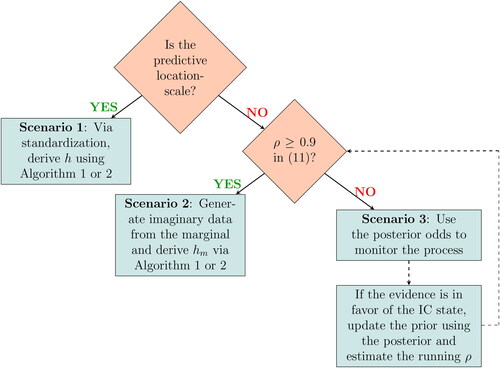We will define as stopping time T of a PRC, tuned for an upward shift: [9] $$T=\inf \{n+1:S_{n+1}\ge h\}$$[9] where $n+1\ge 2,$ except the special case with two unknown parameters and complete prior ignorance, where we have $n+1\ge 3,$ while h > 0 is a preselected constant to guarantee a predetermined false alarm standard (for downward shifts in (9) we have $S_{n+1}\le h,$ with h < 0). The choice of h reflects on the tolerance that we have on false alarms, measured via either the family-wise error rate (FWER), for a fixed and not too long horizon of N data points or the IC average run length (ARL₀), when we have an unknown or a large-N scenario. Due to the general form of PRC’s mechanism, which allows hosting any distribution from the k-PREF, there is no single optimal strategy in selecting h. In what follows, we will provide specific guidelines for the selection of h, utilizing the distributional setup under study. There are three possible scenarios that one can come across in practice: first, when we have a location-scale predictive, second, when the predictive is not a location-scale family distribution but we have an informative prior and, third, when we have neither a location-scale predictive nor an informative prior.

3.1.1. Scenario 1: The predictive is a location-scale family distribution

In this case, we will derive h via the standard predictive distribution (i.e., the distribution with location = 0 and scale = 1). Then, at each step of PRC we will perform the same location-scale transformation to both the IC and OOC predictive distributions, so that each time the IC, $f(X_{n+1}|{\mathit{X}}_n),$ becomes the standard predictive (note that the location-scale transformation will be different at each step). The transformed predictives will be used in the ratio (6). From all the distributions of the regular exponential family shown Table 1 in Bourazas, Sobas, and Tsiamyrtzis (2023) in which PRC schemes were defined, the location-scale predictive is valid for the normal and logarithmic transformed lognormal likelihood cases, where the logarithm of the standardized predictive ratio (6) was tabulated. We provide Algorithms 1 and 2, which can be used to derive via simulations the decision threshold h depending on whether we aim to tune the PRC control chart via either the FWER for a fixed horizon of N data or a target ARL₀ metric, respectively. In addition, in Appendix A (supplementary material) we provide a table with the derived h threshold values for representative choices of (N, FWER) or ARL₀ values, combined with specific OOC shift sizes k, when we have total prior ignorance (i.e., use of initial reference prior and no historical data).

Table 1. The expected ratio of the variance of the likelihood $f(X|\mathit{\theta })$ over the variance of the marginal $f(X|\mathit{Y},{\alpha }_0,\mathit{\tau }),$ defined in (11[11] $$E_{\mathit{\theta }}\left(\frac{\mathit{Var}(X|\mathit{\theta })}{\mathit{Var}(X|\mathit{Y},{\alpha }_0,\mathit{\tau })}\right)=\rho$$[11] ).

Likelihood	Initial prior	Expected ratio (11[11] $$E_{\mathit{\theta }}\left(\frac{\mathit{Var}(X|\mathit{\theta })}{\mathit{Var}(X|\mathit{Y},{\alpha }_0,\mathit{\tau })}\right)=\rho$$[11] )
$f(·|\mathit{\theta })$	${\pi }_0(\mathit{\theta }|\mathit{\tau })$	ρ
P$(\theta ·s_i)$	G(c, d)	$1-\frac{1}{d+{\alpha }_0{\sum }_{j=1}^{n_0}{s}_j+1}$
Bin$(N_i,\theta )$	Beta(a, b)	$1-\frac{N}{a+b+{\alpha }_0{\sum }_{j=1}^{n_0}{N}_j+N}$
NBin$(r,\theta )$	Beta(a, b)	$1-\frac{r}{b+{\alpha }_0{\sum }_{j=1}^{n_0}{y}_j-1+r}$
G$(\alpha ,\theta )$	G(c, d)	$1-\frac{\alpha }{c+\alpha ·({\alpha }_0{n}_0+1)-1}$
W$(\theta ,\kappa )$	$IG(\alpha ,\beta )$	$1-\frac{{\Gamma }^2\left(1+\frac{1}{\kappa }\right)\left[\Gamma (\alpha +{\alpha }_0{n}_0)\Gamma \left(\alpha +{\alpha }_0{n}_0-\frac{2}{\kappa }\right)-{\Gamma }^2\left(\alpha -\frac{1}{\kappa }\right)\right]}{\Gamma (\alpha +{\alpha }_0{n}_0)\Gamma \left(\alpha +{\alpha }_0{n}_0-\frac{2}{\kappa }\right)\Gamma \left(1+\frac{2}{\kappa }\right)-{\Gamma }^2\left(1+\frac{1}{\kappa }\right){\Gamma }^2\left(\alpha -\frac{1}{\kappa }\right)}$
IG$(\alpha ,\theta )$	G(c, d)	$1-\frac{\alpha -2}{c+\alpha ·{\alpha }_0{n}_0-1+\alpha }$
Pa$(m,\theta )$	G(c, d)	$1-\frac{Va{r}_{\theta }\left(\frac{\theta }{\theta -1}\right)}{E_{\theta }(\frac{\theta }{{(\theta -1)}^2(\theta -2)})+Va{r}_{\theta }\left(\frac{\theta }{\theta -1}\right)}$

Algorithm 1

Determine decision threshold (h or h_m) based on FWER

1: Define the length of the data, N, for which PRC will be employed ⊳ initial input

2: Define the FWER that we aim to have at the N-th data point

3: Define the vector ${\mathit{\tau }}_n^{\prime },$ which represents the OOC disturbance that we wish to detect

4: Define the number of iterations, I, used in the empirical estimation

5: if $\{$ predictive distribution is a location-scale family $\}$ then

6: $f(X)=$ the standard distribution ⊳ loc.=0, sc.=1 and $d{f}_n=2{\widehat{a}}_n$ if $X\sim t$

7: else

8: $f(X)=$ the marginal (prior predictive) distribution from (10)

9: end if

10: Generate a matrix D of dimension I × N with random numbers from $f(X)$

11: Set S to be a matrix of dimension I × N filled with zeros

12: Set M to be a vector of dimension I filled with NAs

13: for $\{i$ in $1:I\}$

14: for $\{n$ in $1:(N-1)\}$

15: $L_{n+1}\leftarrow \frac{f\prime (D[i,n+1]|D[i,1],\dots ,D[i,n])}{f(D[i,n+1]|D[i,1],\dots ,D[i,n])}$ ⊳ Predictive ratio

16: $S[i,n+1]=\max \{0,S[i,n]+\log (L_{n+1})\}$

(or S[i,n + 1] = $\min \{0,S[i,n]-\log (L_{n+1})\}$ for downward shifts) ⊳ PRC statistic

17: end for

18: $M[i]\leftarrow \max \{S[i,]\}$

(or $M[i]\leftarrow \min \{S[i,]\}$ for downward shifts)

19: end for

20: $H\leftarrow {\widehat{F}}_I^{-1}(1-\mathit{FWER})$

(or $H\leftarrow {\widehat{F}}_I^{-1}(\mathit{FWER})$ for downward shifts) ⊳ ${\widehat{F}}_I(x)=\frac{1}{I}{\sum }_{i=1}^I\mathbb{1}\left\{M[i]<x\right\}$

21: if $\{$ predictive distribution is a location-scale family $\}$ then

22: $h\leftarrow H$ ⊳ empirical estimate of h

23: else

24: $h_m\leftarrow H$ ⊳ marginal based (conservative) empirical estimate of h

25: end if

Algorithm 2

Determine decision threshold (h or h_m) based on ARL₀

1: Define the ARL₀ that you aim to have

2: Define the numerical tolerance tol, which represents the maximum of error estimate

3: Define the vector ${\mathit{\tau }}_n^{\prime },$ which represents the OOC disturbance that you wish to detect

4: Define the number of iterations I, used in the empirical estimation

5: if {predictive distribution is a location scale family}then

6: $f(X)=$ the standard distribution ⊳ loc.=0, sc.=1 and $d{f}_n=2{\widehat{a}}_n$ if $X\sim t$

7: else

8: f(X) = the marginal (prior predictive) distribution from (10)

9: end if

10: start function ARL(h)

11: Set M to be a vector of dimension I filled with NAs

12: for {i in $1:I$}

13: Set $S\leftarrow 0$

14: Set $n\leftarrow 1$

15: Generate $x_n\sim f(X)$

16: while {S < h (or S > h for downward shifts)}

17: Generate $x_{n+1}\sim f(X)$

18: $L_{n+1}\leftarrow \frac{f\prime (x_{n+1}|x_1,\dots ,x_n)}{f(x_{n+1}|x_1,\dots ,x_n)}$ ⊳ Predictive ratio

19: $S\leftarrow \max \{0,S+\log (L_{n+1})\}$

(or $S\leftarrow \min \{0,S-\log (L_{n+1})\}$ for downward shifts) ⊳ PRC statistic

20: Set $n\leftarrow n+1$

21: end while

22: $M[i]\leftarrow n$

23: end for

24: return {$\mathit{ARL}(h)\leftarrow \overline{M}$} ⊳ $\overline{M}=\frac{1}{I}{\sum }_{i=1}^{I}M[i]$

25: end function ARL(h)

26: Set $h_1=2$ (or $h_1=-2$ for downward shifts) the first initial value for h (or h_m)

27: Get $\mathit{ARL}(h_1)$ ⊳ use of function ARL(h)

28: if {$|\mathit{ARL}(h_1)-AR{L}_0|<\mathit{tol}$}

29: $H\leftarrow h_1$

30: go to 48

31: end if

32: Set $h_2=4$ (or $h_1=-4$ for downward shifts) the second initial value for h (or h_m)

33: Get $\mathit{ARL}(h_2)$ ⊳ use of function ARL(h)

34: if {$|\mathit{ARL}(h_2)-AR{L}_0|<\mathit{tol}$}

35: $H\leftarrow h_2$

36: go to 48

37: end if

38: $H\leftarrow h_2+(AR{L}_0-\mathit{ARL}(h_2))·\frac{(h_2-h_1)}{(\mathit{ARL}(h_2)-\mathit{ARL}(h_1))}$ ⊳ regula falsi estimate

39: Get ARL(H) ⊳ use of function ARL(h)

40: while {$|\mathit{ARL}(H)-AR{L}_0|>\mathit{tol}$}

41: $H\leftarrow h_2+(AR{L}_0-\mathit{ARL}(h_2))·\frac{(h_2-h_1)}{(\mathit{ARL}(h_2)-\mathit{ARL}(h_1))}$ ⊳ regula falsi estimate

42: Get ARL(H) ⊳ use of function ARL(h)

43: $h_1\leftarrow h_2$

44: $h_2\leftarrow H$

45: end while

46: if {predictive distribution is a location scale family}then

47: $h\leftarrow H$ ⊳ empirical estimation

48: else

49: $h_m\leftarrow H$ ⊳ marginal based (conservative) empirical estimation

50: end if

3.1.2. Scenario 2: The predictive is not location-scale family, but we have an informative prior

The posterior predictive remains in closed form, but the unknown parameter(s) and the lack of standardization (because we do not have location-scale family) prevent from deriving a “generator” predictive distribution, as in scenario 1. Our suggestion is to use the marginal (prior predictive) distribution to generate imaginary data. Using the power prior (2), the general form of the marginal distribution will be available in closed form: [10] $$f(X|\mathit{Y},{\alpha }_0,\mathit{\tau })=\underset{\mathit{\Theta }}{\int }f(X|\mathit{\theta })\pi (\mathit{\theta }|\mathit{Y},{\alpha }_0,\mathit{\tau })d\mathit{\theta }=\frac{K\left(\mathit{\tau }+{\alpha }_0{\mathit{t}}_h(\mathit{Y})+{\mathit{t}}_f(X)\right)}{K\left(\mathit{\tau }+{\alpha }_0{\mathit{t}}_h(\mathit{Y})\right)}g(X)$$[10]

The marginal is a compound distribution of the likelihood and the prior, with the unknown parameter(s) being integrated out. It has heavier tails (greater variance) compared to the likelihood, leading to an estimated decision limit $h_m(\ne h)$ that will result a more conservative FWER or ARL₀ metric. Essentially, the likelihood-based threshold h is a limiting case of the marginal-based threshold h_m, when the prior variance tends to zero. Thus, we can generate imaginary data from the marginal, in order to control either the FWER or the ARL₀ and derive the h_m threshold from Algorithms 1 or 2, respectively.

An important issue in this proposal is that the prior needs to be informative; otherwise, the marginal would be too diffused compared to the likelihood, resulting in an upper or lower bound h_m that will be too conservative (i.e., $\left|h_m\right|$ will seriously overestimate $\left|h\right|,$ decreasing significantly the false alarms and the detection power). We propose to measure the discrepancy of the likelihood over the marginal variance by: [11] $$E_{\mathit{\theta }}\left(\frac{\mathit{Var}(X|\mathit{\theta })}{\mathit{Var}(X|\mathit{Y},{\alpha }_0,\mathit{\tau })}\right)=\rho$$[11]

The ratio parameter $\rho \le 1$ expresses the expected underdispersion of the likelihood variance versus the marginal variance. When $\rho \to 1$ (i.e., we use a highly informative prior), then the marginal is a reliable representative of the likelihood, resulting in $h_m\to h.$ After an extensive simulation study, we recommend using the marginal distribution approach only when the distributional setting roughly satisfies $\rho \ge 0.9.$ Table 1 provides the formulas for estimating ρ for each of the PRC models reported in Table 1 of Bourazas, Sobas, and Tsiamyrtzis (2023; that do not fall in the location-scale family treated by scenario 1), where for the power prior term, we assume the historical data $\mathit{Y}=(y_1,\dots ,y_{n_0}),$ which are weighted by α₀ (for no historical data, set ${\alpha }_0=0$).

In Appendix B (supplementary material), we provide some illustration of the achieved FWER and ARL₀ based on h_m, as a function of ρ for different parameter values when we have Poisson or binomial likelihoods.

3.1.3. Scenario 3: The predictive is not location-scale family and we do not have an informative prior

When our distributional setup does not conform with either scenario 1 or 2, we face the most challenging case. Because we do not have a reliable way to estimate h using imaginary data, we will make use of the predictive Bayes factor to form some evidence-based limits for the charting statistics $S_{n+1}.$ In (8) we expressed $S_{n+1}$ as the zero truncated cumulative logarithmic Bayes factor, which measures the evidence of the alternative model ${\mathcal{M}}_1$ (OOC) against the null ${\mathcal{M}}_0$ (IC). In addition, under the assumption that the IC and OOC models are equally probable a priori, i.e., $P({\mathcal{M}}_0)=P({\mathcal{M}}_1),$ then $B_{10}^{n+1}$ is simply the posterior odds of the two models. Kass and Raftery (1995), following Jeffreys (1961), provided an analytical interpretation of $B_{10}^{n+1}$ and offered threshold values for decision-making. Based on these guidelines, when $B_{10}^{n+1}>100,$ then the evidence against the null model is referred as “decisive” because the posterior probability of the alternative model will be at least 100 times greater than the corresponding of the null. Thus, we recommend using $h_J=\log (100)\approx 4.605$ as an evidence based limit for $S_{n+1}.$ In other words, if $S_{n+1}>h_J$ (or $S_{n+1}<-h_J$ for downward shifts), then we have a decisive cumulative evidence in favor of the OOC state.

The evidence-based limits can be used for a few initial steps to monitor the process. At each step, as long as the posterior odds reveal that we are in the IC state, we can use the obtained data to update the prior setting (because the posterior at each time point acts as prior for the next observable) and examine whether it becomes informative (based on ρ) or not. Once we have an informative prior, we move to scenario 2, generating imaginary data from the marginal and deriving h_m, initiating a new PRC.

In Figure 1, we summarize all the proposed options for deriving a PRC’s decision threshold. The threshold h will depend on the likelihood of the data, the prior settings, and the intervened vector ${\mathit{\tau }}_{\mathit{n}}^{\prime },$ with the latter reflecting the discrepancy between the current (IC) and the intervened (OOC) distribution. In general, assuming that the deviation between IC and OOC state is considerably large, then if a change of smaller size occurs, PRC might absorb it. On the other hand, if the real shift is greater than the one we have set, then PRC probably will have a slightly delayed alarm, but it is expected to react. Therefore, the choice of the OOC state must take into account the absorption risk, avoiding setting PRC for very large shifts (a similar discussion regarding SSC can be found in Zantek 2006). This is an issue, closely related with West’s (1986) CBF methodology where the alternatives are set to be diffused, allowing potentially large shifts, a strategy that has a high risk in absorbing small shifts and not reacting on them (for more information, refer to Section 4 where the relative performance and the robustness of these methods are extensively examined).

Figure 1. Determining the decision threshold h for a predictive ratio cusum (PRC) scheme. A decision is represented by a rhombus, and a rectangle corresponds to an operation after a decision is made.

Quite often in practice, we might need to employ more than a single PRC, like when we monitor the mean of a normal distribution for either an upward or a downward shift. In such cases, we need to account for the multiple testing, and so if we use the FWER metric we simply need to adjust its value, using, for example, Bonferroni’s correction (Dunn 1961). For the ARL metric, one can refer to Hawkins and Olwell (1998), among others, on how to combine the individual CUSUM ARLs in getting a designed overall ARL.

3.2. Fast initial response (FIR) PRC

It is well known that the self-starting memory-based charts have a weak response to shifts arriving early in the process. Failing to react to an early shift will lead to its absorption, contaminating the calibration and reducing the testing performance. Lucas and Crosier (1982) were the first to introduce the fast initial response (FIR) feature for CUSUM by adding a constant value to the initial cumulative statistic, enhancing its reaction to very early shifts in the process. Steiner (1999) introduced the FIR Exponentially Weighted Moving Average (EWMA) by narrowing its control limits, with the effect of this adjustment decreasing exponentially fast. For PRC, we propose an exponentially decreasing adjustment, multiplied to the statistic $\log (L_{n+1}).$ Specifically, the adjustment (inflation) will be: [12] $${\text{FIR}}_{\mathit{adj}}=1+f·d^{(t-1)},$$[12] where t is the time of the examined predictive ratio, $f\ge 0$ represents the proportion of the inflation for the PRC statistic, $\log (L_{n+1}),$ when t = 1 and $0<d<1$ is a smoothing parameter, specifying the exponential decay of the adjustment (the smaller the d the fastest the decay). As the first predictive ratio is available for the second observation, we have t = 1 when n = 2. The only exception is when we have two unknown parameters and total prior ignorance (i.e., use of initial reference prior and ${\alpha }_0=0$ due to lack of historical data), where we get t = 1 when n = 3.

The proposed FIR adjustment is more flexible compared to the fixed constant of Lucas and Crosier (1982), FIR-CUSUM, as it allows to control the influence, by tuning the initial parameters (f, d), providing a better interpretation. The FIR option can improve the performance at the early start, but the choice of the adjustment parameters must be prudent, avoiding significant inflation of the false alarm rate. The expected number of false alarms for PRC will depend on the prior settings, especially when the volume of available data is small. In general, the choice of f will correspond to the inflation that we wish to have at the start of the monitoring (t = 1). As a rule of thumb, f could be selected so that after the first test ($n+1=2$) and assuming that $\log (L_2)<h$ (i.e., we do not have an alarm), then $f=(h-\log (L_2))/2;$ that is, the inflation is such that it boosts up the monitoring statistics, reaching halfway from where it was to the decision threshold h. This strategy will guarantee that we will not get an alarm due to adjustment setting at the first test. Of course, a different choice will reflect a different policy, but the general recommendation is to avoid too large values as they will increase significantly the risk of a false alarm. The parameter d, on the other hand, will express the rate of decrease of the adjustment. Precisely, specifying the time $t^{*}$ where we wish the inflation to be reduced to just $a^{*}$ then $a^{*}=f·d^{(t^{*}-1)},$ and thus we get: [13] $$d=\exp \left\{\frac{\log (a^{*})-\log (f)}{t^{*}-1}\right\}$$[13]

Our suggestion is to be somewhat conservative, especially when a weakly informative prior is used, so that the FIR adjustment will not seriously affect the predetermined expected number of false alarms. A recommendation that we will follow throughout this work is to use $(f,d)=(1/2,3/4),$ where the adjusted $\log (L_{n+1})$ will be inflated by $f=50\%$ for the first test, while the inflation will be $a^{*}=5\%$ at the $t^{*}=9$ th test (the choice of these parameters will reflect the user’s based needs). Because for scenarios 2 and 3 in determining the decision threshold, we will have h_m to be a more conservative estimate, resulting in lower false alarms (from what we design), the use of FIR-PRC is motivated. Additionally, in some cases of handling big values of ARL₀, the FIR adjustment might be implemented for longer periods of data and not just for the very few first observations. Figure 10 in Appendix B (supplementary material) visualizes the benefit of FIR-PRC when h_m is used, while Appendix C (supplementary material) evaluates its performance for shifts occurring early in the process (the performance metrics used are defined in Section 4).

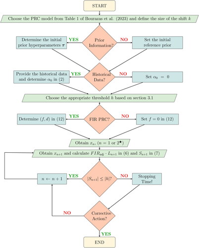
The PRC’s flowchart and pseudo-algorithm that were presented in Bourazas, Sobas, and Tsiamyrtzis (2023) are extended to include the new design concepts of the decision interval h and FIR options and presented here in Figure 2 and Appendix D (supplementary material), respectively.

Figure 2. Predictive ratio cusum (PRC) flowchart 2. A parallelogram corresponds to an input/output information, a decision is represented by a rhombus, and a rectangle denotes an operation after a decision-making. In addition, the rounded rectangles indicate the beginning and end of the process. *For the likelihoods with two unknown parameters and total prior ignorance (i.e., initial reference prior and ${\alpha }_0=0$ in the power prior), we need n = 3 to initiate PRC, while for all other cases, PRC starts right after x₁ becomes available.

4. PRC robustness study

The PRC, much like any other parametric-type statistical method, imposes certain modeling assumptions. In the simulation study presented by Bourazas, Sobas, and Tsiamyrtzis (2023), it was shown that when these assumptions are valid, PRC outperforms its competitors SSC and CBF. What happens, though, when we encounter violations of these assumptions? In this section, we will extend the simulation study of Bourazas, Sobas, and Tsiamyrtzis (2023) by examining how robust the performance of PRC and its competing methods is when we experience various model type misspecifications.

First, we will provide the simulation setting and the performance metrics that were used in Bourazas, Sobas, and Tsiamyrtzis (2023) and will be adopted here as well. For each model setting assumed, we tune all competing methods to have identical false alarm rate and to be designed appropriately to detect the assumed OOC scenario under study. To derive the decision limit of each method, we simulate 100,000 IC sequences of size N = 50 observations from $N({\theta }_1=0,{\theta }_2^2=1)$ (that will be used for both the mean and the variance charts) and $P({\theta }_3=1).$ For the priors used by the Bayesian methods (PRC and CBF), we will consider the scenarios of absence/presence of prior information using as initial priors ${\pi }_0(·|\mathit{\tau }):$

• Normal: reference (non-informative) prior ${\pi }_0({\theta }_1,{\theta }_2^2)\propto 1/{\theta }_2^2\equiv \mathit{NIG}(0,0,-1/2,0)$ or the moderately informative $\mathit{NIG}(0,4,2,1.5).$

• Poisson: reference (non-informative) prior ${\pi }_0({\theta }_3)\propto 1/\sqrt{{\theta }_3}\equiv G(1/2,0)$ or the moderately informative G(4, 4).

The OOC scenarios will represent a persistent parameter shift of medium/small size introduced at one of the locations $\omega =\{11,26\mathrm{ }\text{or}\mathrm{ }41\}$ out of the N = 50 observations. Regarding the performance metrics, we start by tuning all methods to have 5% family-wise error rate (FWER) when we have IC data of length 50, i.e., $\mathit{FWER}(N)=P(T\le N|\omega >N)=0.05,$ where T denotes the stopping time, ω is the time of the step change and N = 50 (length of the data in this study). To measure the power, we will use the probability of successful detection (PSD, Frisén 1992), where $\mathit{PSD}(\omega )=P(\omega \le T\le N),$ where the bigger the $\mathit{PSD}(\omega ),$ the better. The other important metric in persistent shift detection is the delay in ringing the alarm, which here will be evaluated via the truncated conditional expected delay, i.e., $\mathit{tCED}(\omega )=E(T-\omega +1|\omega \le T\le N)$ (Kenett and Pollak 2012), and it is the average delay of the stopping time, given that this stopping time was after the change point occurrence and before the end of the sample (i.e., point of truncation), so the smaller the delay, the better the performance. In what follows, we will examine the robustness of PRC, SSC, and CBF in IC and OOC data streams when we experience four different types of modeling violations.

1. Likelihood misspecifications, with three cases, where we:

   • Tune all methods in detecting mean shifts of a normal likelihood, but simulate the data streams from the heavy-tailed Student - t₅ distribution.

   • Tune all methods in detecting mean shifts of a normal likelihood, but simulate the data streams from the right skewed $\mathit{Gumbel}(\mu =-0.5,\beta =0.8)$ distribution.

   • Tune all methods for a shift in a Poisson likelihood, but simulate the data streams from the overdispersed $\mathit{NBin}(r=4,p=1/5)$ distribution.

For all above cases, the OOC data will refer to the simulating distribution that undergoes a parameter shift of size 1 SD.

• b. OOC state misspecifications, where we will tune all the methods for detecting a step change of size $1\sigma$ in the mean of normal data, but the simulated OOC scenario will correspond to one of the following three cases:

  • $0.5\sigma$ mean shift (i.e., the OOC shift size is smaller from what we designed)

  • $1.5\sigma$ mean shift (i.e., the OOC shift size is bigger from what we designed)

  • 100% inflation of σ (i.e., we misspecified the type of change).

• c. Prior misplacement. In the Bayesian approach and in particular in real-life applications, users are often concerned of the risk in selecting an “inappropriate” prior. A strategy to break free from a prior selection and still use a Bayesian approach is to have an objective analysis, where among others, a flat (uniform) prior, Jeffreys (1961) prior or a reference prior (Bernardo 1979; Berger, Bernardo, and Sun 2009) is employed. Within the prior sensitivity analysis performed in Bourazas, Sobas, and Tsiamyrtzis (2023), though, the effect of using a moderately informative prior distribution versus the objective choice of a reference prior was examined for the Bayesian methods of PRC and CBF, and it was observed (as expected) that the moderately informative prior has higher detection power compared to the reference prior. Thus, if prior information exists, then it is recommended to be used in the Bayesian scheme. The proposal is to avoid to have highly informative priors (i.e., priors with support on a very “narrow” region of the parameter space) as in such cases there is a risk to have what is known as prior-likelihood conflict, where the prior probability is vastly concentrated over low density areas of the likelihood. For the issue of prior-data conflict one can refer, among others, to Evans and Moshonov (2006), Bousquet (2008), Evans and Jang (2011), Al Labadi and Evans (2017), and Egidi, Pauli, and Torelli (2022). In Bayesian control charts, a highly informative prior properly allocated will provide top performance results, while if it is misplaced will give rise to prior data conflict resulting in an inappropriate false alarm rate. To mitigate the prior data conflict risk, our proposal is to select moderately (as opposed to highly) informative priors, that is, priors with larger variance. The next question is what happens when a moderately informative prior is not properly located. In this scenario, we will test how robust the performance of PRC and CBF is when the moderately informative priors are not accurately located. Precisely, we will set the processes for detecting mean step changes of size $1\sigma$ when the IC data are from a N(0, 1). The moderately informative prior for this case, used in Bourazas, Sobas, and Tsiamyrtzis (2023), was $\mathit{NIG}({\mu }_0,4,2,1.5)$ with prior mean ${\mu }_0=0,$ that is, at the value of the unknown parameter. Keeping all but μ₀ parameters of the NIG prior the same, we will examine the effect of the prior misplacement. Specifically, we will examine two cases:

  • $\mathit{NIG}(0.5,4,2,1.5)$ with prior mean ${\mu }_0=0.5,$

  • $\mathit{NIG}(-0.5,4,2,1.5)$ with prior mean ${\mu }_0=-0.5.$

• d. Independence violation. In PRC, as in most of the traditional SPC/M methods, the data are assumed to be independently sampled. In this scenario, we will examine the performance when the data exhibit autocorrelation. Precisely, we assume that we have a PRC for normal independent data but the simulated IC data are from an AR(1) model: $X_{n+1}=\varphi X_n+ϵ,$ with $ϵ\sim N(0,1)$ where:

  • $\varphi =0.3,$ or

  • $\varphi =-0.3$

We will examine the performance when we experience jumps of size 1 SD for the mean or 50% inflation for the standard deviation.

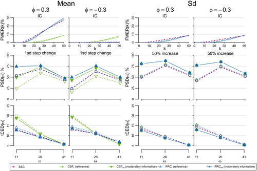
Figures 3–6 provide a graphical representation of the robustness results for scenarios (a)–(d) respectively, while Tables 7–10 in Appendix E (supplementary material) tabulate the corresponding results. The reference (baseline) performance, where no assumption is violated, was presented in Bourazas, Sobas, and Tsiamyrtzis (2023).

Figure 3. The family-wise error rate FWER(k) at each time point $k=2,3,\dots ,50,$ the probability of successful detection, probability of successful detection $\mathit{PSD}(\omega )$ and the truncated conditional expected delay, truncated conditional expected delay $\mathit{tCED}(\omega )$ for shifts at locations $\omega =\{11,26,41\},$ of self-starting cusum SSC, cumulative Bayes factor CBF and PRC, under a reference (CBF_r, PRC_r) or a moderately informative (CBF_mi, PRC_mi) prior for OOC scenarios with misspecified likelihood. All the procedures are set for a mean step change size of $1\sigma$ in data from a standard Normal or an rate increase of 50% in P(1) data.

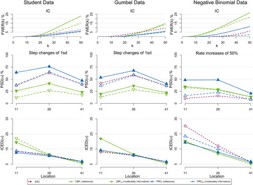
Figure 4. The $\mathit{PSD}(\omega )$ and $\mathit{tCED}(\omega )$ for shifts at locations $\omega =\{11,26,41\},$ of SSC, CBF and PRC, under a reference (CBF_r, PRC_r) or a moderately informative (CBF_mi, PRC_mi) prior for OOC scenarios with misspecified jumps. All the procedures are set for a mean step change of size $1\sigma$ in data from a standard normal distribution.

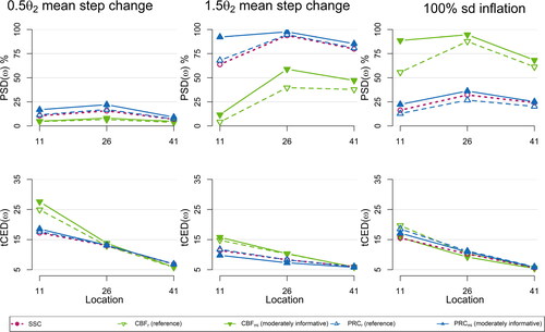
Figure 5. The FWER(k) at each time point $k=2,3,\dots ,50,$ $\mathit{PSD}(\omega )$ and $\mathit{tCED}(\omega )$ for shifts at locations $\omega =\{11,26,41\},$ of PRC under two misplaced moderately informative priors in the negative and positive directions ($PR{C}_{-}$ and $PR{C}_{+}$ respectively), along with the and CBF under the same priors ($CB{F}_{-}$ and $CB{F}_{+}$). All the methods are set for detecting a positive mean step change of size $1\sigma$ in normal data.

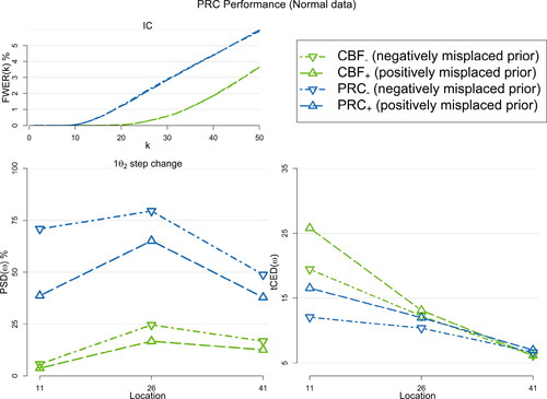
Figure 6. The $\mathit{PSD}(\omega )$ and $\mathit{tCED}(\omega )$ for shifts at locations $\omega =\{11,26,41\},$ of SSC, CBF, and PRC, under a reference (CBF_r, PRC_r) or a moderately informative (CBF_mi, PRC_mi) prior for OOC scenarios with dependent data. All the procedures are set for a mean step change of size $1\sigma$ for the mean or 50% inflation for the standard deviation in data from a standard normal distribution.

For (a), in Figure 3 we observe that PRC is less affected by likelihood violations in either the false alarms of IC sequence or the detection power in the OOC scenarios. Specifically, the false alarms of SSC and CBF become unacceptably high in most cases, while those of PRC are close to the predetermined level, particularly with the reference prior, where PRC is almost unaffected. PRC has greater detection percentages from SSC and CBF, especially using the moderately informative prior. We should note that the reported improved detection performance of SSC and CBF should be considered with caution as the associated false alarm rate is significantly higher in these cases.

Regarding (b), where the shift size for the OOC scenario is misspecified (Figure 4), we observe that PRC is still dominating both SSC and CBF. Comparing against the reference performance where all assumptions were valid, we observe that now it is somewhat decreased/increased if the shift size is smaller/larger from what PRC was tuned for. Seemingly, the only exception regarding PRC’s dominance is in the case of using a scheme that looks for a mean shift, while in practice we have a change in variance. There, the CBF has a superior performance, but this was expected, as CBF is essentially a method that can successfully detect changes in variance. However, as was shown in Bourazas, Sobas, and Tsiamyrtzis (2023), the CBF is identical to the PRC for variance shifts and thus the exact same performance would be provided by a suitably set PRC for variance shifts.

For scenario (c), in Figure 5 we observe that PRC is quite robust (significantly outperforming the CBF), when the moderately informative prior distribution is mislocated. Notably, this is valid, even for the $PR{C}_{+}$ where the prior distribution is on the same direction to the jump (i.e., ${\mu }_0=+0.5$) leading to a more extensive overlap the IC and OOC predictive distributions.

Finally, for scenario (d), in Figure 6 we have that in the case of variance shifts or mean shift with negative autocorrelation the performance is quite robust. In contrast, when we have a positive mean shift and positive autocorrelation, both the PRC and SSC have a very high FWER compared to the designed level, being the only exception in a solid performance. This handicap was somewhat expected and can be attributed to the CUSUM’s sensitivity to autocorrelation (see, e.g., Hawkins and Olwell 1998). In the cases where high autocorrelation is present, it is suggested first to apply a time series model to remove it and then use PRC on the residuals, much like it is recommended in various other SPC/M methods.

As a synopsis, the PRC appears to have a quite robust performance in the presence of various model type misspecifications, dominating both in terms of false alarm behavior and detection power its competing methods in the vast majority of the scenarios tested. This is of great importance, especially regarding the use of PRC in everyday practice, where it is not uncommon to experience model assumption violations.

5. Real data application

In this section, we will illustrate the use of PRC in real data. In particular, we will apply the developed methodology in three real datasets (one for continuous and two for discrete data). Regarding the continuous case, which motivated the development of PRC, we will use data that come from the daily Internal Quality Control (IQC) routine of a medical laboratory and specifically from the area of hemostasis discipline. We are interested in the variable “Factor V,” measured in percentage regarding the international standards in Biology (National Institute for Biological Standards and Control). Factor V is one of the serine protease enzymes of the procoagulant system, which interacts on a phospholipid surface to induce formation of stable clot of fibrin. Deficiencies of Factor V can induce bleeding disorders of varying severity. The normal range for factor V level is 61% to 142% (for adults), and in this application we focus on pathological values (i.e., measurements below 60%, which biologists call abnormal values). In a medical laboratory, where control samples are used to monitor the quality of the process, it is known that a change of reagent batch (i.e., change between two successive batches) might introduce a step change to the measurement of Factor V. This can occur at the early stages of the process, and it is crucial to identify such a change point, when present, to avoid clinically impacting the patient’s care. We sequentially gathered 21 normally distributed IQC observations (X_i) from a medical laboratory (see Table 2), where $X_i|({\theta }_1,{\theta }_2{}^2)\sim N({\theta }_1,{\theta }_2{}^2).$

Table 2. The Factor V (%) internal quality control observations of the current $\mathit{X}=(x_1,x_2,\dots ,x_{21})$ data, reported during September 24, 2019–October 8, 2019.

$x_1-x_{11}$	31.0	30.0	32.0	28.0	33.2	33.2	35.1	35.1	33.9	37.9	33.2
$x_{12}-x_{21}$	36.5	33.2	35.1	34.5	36.5	33.2	35.1	37.2	32.6	36.5

From the control sample manufacturer, we elicit the initial prior ${\pi }_0({\theta }_1,{\theta }_2{}^2|\mathit{\tau })\sim \mathit{NIG}(31.8,1/2,2,4.41).$ Furthermore, we have $n_0=37$ IC historical data (from a different reagent) available, with $\overline{\mathbf{y}}=31.73$ and $\mathit{var}(\mathbf{y})=3.31$ and we set ${\alpha }_0=1/37$ in the power prior term to convey the weight of a single data point to these. Combining the two sources of information within the power prior (2) we obtain: $\pi ({\theta }_1,{\theta }_2{}^2|\mathit{Y},{\alpha }_0,\mathit{\tau })\sim \mathit{NIG}(31.75,3/2,5/2,6.02).$ The goal is to detect any small persistent positive or negative shift in the mean of the process, as this will have an impact on the reported patient results. The concept of small is expressed in terms of a multiples of the standard deviation and so in this setup, we choose the parameter k = 1, that is, we look for persistent shifts of magnitude 1 SD, as at low levels of Factor V the bleeding risk can hugely increase with small differences. Thus, we tune the PRC in detecting mean step changes, in either upward or downward direction, of 1 SD size (i.e., $\pm {\widehat{\theta }}_2$). The PRC control chart will plot two monitoring statistics: $S_{n+1}^{+}$ (evolving in the nonnegative part) and $S_{n+1}^{-}$ (evolving in the nonpositive numbers) that will test for upward and downward persistent mean shifts, respectively. Furthermore, we will have two decision limits, h⁺ and h^–, which due to the normal distribution symmetry and the design of the same OOC step change shift ($\pm {\widehat{\theta }}_2$) will be of the same magnitude (i.e., $\left|h^{+}\right|=\left|h^{-}\right|$). 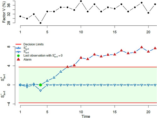As the data are normally distributed, the standardized version of PRC is available and from scenario 1 of Section 3.1.1 we derive the decision limit $h^{+}=3.749$ ($h^{-}=-3.749$) to achieve $\mathit{FWER}=10\%$ for 21 observations (because we run two tests we used Bonferroni’s adjustment resulting $\mathit{FWER}=5\%$ for each of the PRCs). As this study is offline, we will not interrupt the process after a PRC alarm (as we would have done when PRC runs online), but instead we will let it run until the end of the sample in order to perceive its behavior in the presence of contaminated data.

Figure 7 provides the two-sided PRC chart along with the plot of the available data. The control chart rings an alarm at location eight indicating an upward mean shift, which seems to be initiated right after location four (i.e., last time where $S_{n+1}^{+}=0$ before the alarm), that is, ω = 5 and we have a delay of three observations in ringing the alarm. It is worth noting also that the alarm persists until the end of the sample, indicating PRC’s resistance in absorbing the change. Regarding the self-starting methods SCC and CBF, we should note that when applied in real problems with unknown parameter values, they both lack the ability to derive an appropriate decision threshold that will respect a predetermined FWER, making their use in everyday practice prohibitive.

Figure 7. Predictive ratio cusum (PRC) for normal data. At the top panel, the data are plotted, while at the lower panel, we provide the PRC control chart, focused on detecting an upward or downward mean step change of one standard deviation size, when we aim a $\mathit{FWER}=10\%$ for 21 observations.

Next, we provide the PRC’s illustration for Poisson data, presented initially by Dong, Hedayat, and Sinha (2008) and analyzed by Ryan and Woodall (2010) as well. They refer to counts of adverse events (x_i), per product exposure in millions (s_i), in a pharmaceutical company. We have 22 counts (see Table 3) arriving sequentially that we will model using the Poisson distribution with unknown rate parameter, that is, $X_i|\theta \sim P(\theta ·s_i).$ In contrast to the previous application, neither prior information regarding the unknown parameter nor historical data exist. Therefore, we use the reference prior as initial prior for θ, that is, ${\pi }_0(\theta |\mathit{\tau })\propto 1/\sqrt{\theta }\equiv G(1/2,0)$ and we also set ${\alpha }_0=0$ for the power prior term.

Table 3. Counts of adverse events (x_i) and product exposure (s_i) per million ($i=1,2,\dots ,22$), for each quarter reported during July 1, 1999–December 31, 2004 (see Dong, Hedayat, and Sinha 2008).

Adverse events $(x_1-x_{11})$	1	0	0	0	1	0	3	3	3	2	5
Product exposure $(s_1-s_{11})$	0.206	0.313	0.368	0.678	0.974	0.927	0.814	0.696	0.659	0.775	0.731
Adverse events $(x_{12}-x_{22})$	5	2	4	4	3	4	3	8	3	2	2
Product exposure $(s_{12}-s_{22})$	0.710	0.705	0.754	0.682	0.686	0.763	0.833	0.738	0.741	0.843	0.792

We tune PRC in detecting a 100% increase in the rate parameter and we also provide the FIR-PRC version, setting $(f,d)=(1/2,3/4).$ As the predictive distribution is not a location/scale family and the prior is not informative, we fall under scenario 3 of Section 3.1.3, and so we will make use of the evidence-based threshold $h_J=\log (100)\approx 4.605.$ Just as we did in the previous application, we will analyze all the data in an offline version and not interrupt the process after an alarm to record the alarm’s persistence. In Figure 8, a plot of the data along with the two versions of PRC (with/without FIR) are provided.

Figure 8. Predictive ratio cusum (PRC) for Poisson data. At the top panel, we plot the counts of adverse events x_i (solid line) and the rate of adverse events per million units $x_i/s_i$ (dashed line). At the lower panel, we provide the PRC control chart, focused on detecting 100% rate inflation and the evidence based limit of $h_J=\log (100)\approx 4.605$ is used. For the fast initial response (FIR)-PRC (dashed line) the parameters $(f,d)=(1/2,3/4)$ were used.

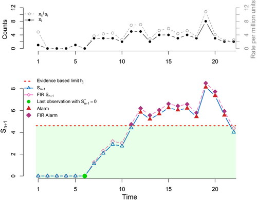
The PRC provides the first alarm at observation 12, while the FIR-PRC gives an alarm at location 11, both indicating that we had a persistent rate increase, which appears to have started right after location six. Location six was the last time before the alarm where the monitoring statistic was zero. Furthermore, the alarm persists until observation 21, after which the monitoring statistics returns to the IC region. It is worth mentioning that, because we have a decisive evidence that the procedure is OOC, we maintained the evidence limit until the end of the sample, avoiding the option of deriving h_m via the marginal distribution after the first few data, as described in scenario 3 of Section 3.1.3. We also note that both in Dong, Hedayat, and Sinha (2008) and Ryan and Woodall (2010), where the aim was to have an IC Average Run Length $AR{L}_0\approx 100,$ their cumulative evidence monitoring approach gave only a single alarm at location 19 (i.e., the alarm comes later compared to PRC and is absorbed instantly). We complete this section by providing the PRC’s application to binomial data, using a dataset from Huang, Reynolds, and Wang (2012), originally presented by Pruett and Schneider (1993). The data refer to the shipping papers that label shipping goods and record information about the buyer. When a shipping paper contains incorrect or missing information about a buyer is classified as “defective” because it will result a delay in the shipping process. For a period of 40 days, a sample of 50 shipping papers was inspected daily and the number of defective papers found was recorded (Table 4). If we denote as θ the probability of a shipping paper to be defective, then for the observed data we assume $X_i|\theta \sim \mathit{Bin}(50,\theta ),i=1,2,\dots ,40.$

Table 4. The sequence of the data $\mathit{X}=(x_1,x_2,\dots ,x_{40}),$ representing the number of defective per 50 sampled shipping papers.

$x_1-x_{20}$	3	3	1	5	2	1	3	3	3	0	2	1	2	1	4	1	1	0	3	2
$x_{21}-x_{40}$	4	6	0	1	3	2	2	4	2	1	2	4	5	2	4	8	4	4	8	5

In the absence of any prior information in Huang, Reynolds, and Wang (2012), the course of action was to reserve the first 30 observations as phase I data, which were used to calibrate the control chart. Then they examined retrospectively the first 30 data points, where no alarm was present, and they analyzed the last 10 data points as phase II, receiving consecutive alarms from point 36 until 40, tracing the change point at location 31.

We will implement the PRC methodology on the same data. Due to the lack of any prior information or historical data, we employ as initial prior for the probability of a label being defective (θ), the reference prior, i.e., ${\pi }_0(\theta )=\mathit{Beta}(1/2,1/2),$ while we set ${\alpha }_0=0$ for the power prior parameter. Furthermore, we tune the PRC to detect a 100% increase in the odds of θ. As PRC is a self-starting approach, it will be able to provide online inference from the start of data collection, with no need of employing a phase I exercise. Due to the absence of any prior information we are under scenario 3 of Section 3.1.3 and so we will use the evidence based limit $h_J=\log (100)\approx 4.605.$ For the first 30 data points, we do not have any alarm (see Figure 9), just as in Huang, Reynolds, and Wang (2012), but with the basic difference that PRC performed the testing in an online fashion.

Figure 9. Predictive ratio cusum (PRC) for binomial data. At the top panel, we plot the number of defective shipping papers x_i, while at the lower panel, we provide the PRC control chart, focused on detecting 100% odds inflation. The evidence based limit of $h_J=\log (100)\approx 4.605$ is used for the first 30 observations, and then these data are used for the derivation of the decision limit $h_m=4.332,$ setting the average run length ${\mathrm{ARL}}_0=400.$

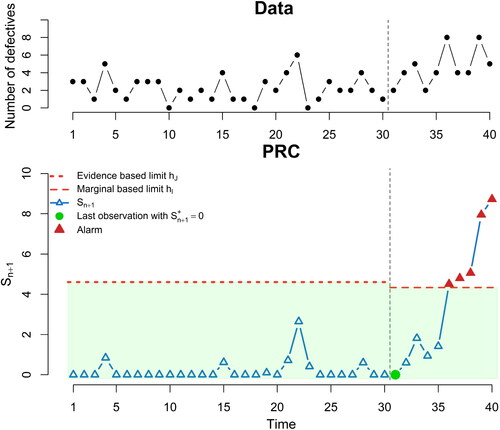
At the 30th data point, the posterior distribution for θ is a $\mathit{Beta}(66.5,1434.5).$ This will play the role of the prior in deriving the marginal (predictive) distribution in (10), resulting a $\mathit{BetaBin}(66.5,1434.5,50).$ Then, the expected ratio parameter ρ from (11) can be estimated (see Table 1) to be $\rho \approx 0.968.$ This relatively large value (compared to the empirical 0.9 value suggested in Section 3.1), supports that the marginal is a reliable representative of the likelihood and so from the flowchart in Figure 1, we can generate imaginary data. Setting $AR{L}_0=400$ (similar to Huang, Reynolds, and Wang 2012) from the imaginary data we derive the decision limit $h_m=4.332.$ Restarting the PRC at time 31 with the new decision limit and running it online until the end of the data, we receive 5 alarms, starting from observation 36 until the end of the sample, with the change point being identified at location 31 (see Figure 9), identical to the findings of Huang, Reynolds, and Wang (2012).

6. Conclusions

Self-starting methods offer the flexibility to have online inference from the start of the process, with no need to have a phase I calibration step. These methods, though, face a big challenge when one wishes to apply them in practice. Precisely, it is difficult to tune such a method to guarantee a predetermined false alarm tolerance, as for the IC state distribution the involved parameters are unknown and sequentially updated.

In this work, we focus in the PRC control chart (suitable for detecting persistent parameter shifts), and we propose a protocol that derives a decision-making threshold, based on the desired false alarm tolerance, something that is generally missing in the literature, especially when we deal with non-normal data. The methodology utilizes the Bayesian framework and is capable of providing exact (h) or approximate (h_m) decision-making limit, depending on the likelihood used and the available prior information. In the cases of total prior ignorance (reminiscent of the frequentist approach), a conservative evidence-based limit (h_J) is proposed, until the incoming data provide sufficient information to form an informative posterior distribution.

Additionally, the fast initial response (FIR) feature for PRC was introduced, and its study showed that it can enhance the PRC performance, when we have shifts that arrive at the early stages of the process. A detailed simulation study indicated that PRC is quite robust when different model-type assumption violations occur, outperforming SSC and CBF in most of the cases tested, a result of high interest to practitioners.

The PRC defines a Bayesian framework, where possibly available prior information and/or historical data can be incorporated, enhancing the performance and providing a setup where one can derive a decision making limit based on the required false alarm tolerance. PRC is quite general, covering a big variety of discrete and continuous distributions used in SPC/M and is capable of running even under total prior ignorance scenarios. The closed form monitoring procedure, along with the availability of an associated decision-making limit (typically absent in standard competing methods) based on the false alarm policy that one wishes to have, allows its straightforward implementation in practice for either short (using FWER) or long (via ARL₀) sequences of data.

Acknowledgments

We are grateful to the editor and all reviewers for their excellent work. Their constructive criticism and suggestions significantly improved the quality of this manuscript.

Additional information

Funding

This research was partially funded by the international company Instrumentation Laboratory (IL), Bedford, Massachusetts, USA and the Research Center of the Athens University of Economics and Business (RC/AUEB).

Notes on contributors

Konstantinos Bourazas

Dr. Konstantinos Bourazas received his Ph.D. from the Department of Statistics, at the Athens University of Economics and Business, Greece. He is currently a postdoctoral researcher at the Department of Mathematics & Statistics at the University of Cyprus, as well as participating in an interdepartmental research project at the University of Ioannina, Greece. His research interests are in the areas of Statistical Process Control and Monitoring, Bayesian Statistics, Change Point Models, Replication Studies and Applied Statistics. is specialized in hemostasis. He is a clinical chemist graduated from Claude Bernard University Lyon I, France. He is a Quality Manager focusing in medical laboratories accreditation issues with respect to ISO 15189 norm.

Frederic Sobas

Panagiotis Tsiamyrtzis is an Associate Professor at the Department of Mechanical Engineering, Politecnico di Milano and his email is [email protected].

References

- Al Labadi, L., and M. Evans. 2017. Optimal robustness results for relative belief inferences and the relationship to prior-data conflict. Bayesian Analysis 12 (3):705–28. doi: 10.1214/16-BA1024.
- Berger, J. O., J. M. Bernardo, and D. Sun. 2009. The formal definition of reference priors. Annals of Statistics 37:905–38.
- Bernardo, J. M. 1979. Reference posterior distributions for Bayesian inference. Journal of the Royal Statistical Society Series B (Methodological) 41 (2):113–28. doi: 10.1111/j.2517-6161.1979.tb01066.x.
- Bourazas, K., F. Sobas, and P. Tsiamyrtzis. 2023. Predictive Ratio Cusum (PRC): A Bayesian approach in online change point detection of short runs. Journal of Quality Technology, online advance. doi: 10.1080/00224065.2022.2161434.
- Bousquet, N. 2008. Diagnostics of prior-data agreement in applied Bayesian analysis. Journal of Applied Statistics 35 (9):1011–29. doi: 10.1080/02664760802192981.
- Brook, D., and D. A. Evans. 1972. An approach to the probability distribution of CUSUM run length. Biometrika 59 (3):539–49. doi: 10.1093/biomet/59.3.539.
- Deming, W. E. 1986. Out of Crisis. Cambridge, MA: The MIT Press.
- Dong, Y., A. S. Hedayat, and B. K. Sinha. 2008. Surveillance strategies for detecting change point in incidence rate based on exponentially weighted moving average methods. Journal of the American Statistical Association 103 (482):843–53. doi: 10.1198/016214508000000166.
- Dunn, O. J. 1961. Multiple comparisons among means. Journal of the American Statistical Association 56 (293):52–64. doi: 10.1080/01621459.1961.10482090.
- Egidi, L., F. Pauli, and N. Torelli. 2022. Avoiding prior-data conflict in regression models via mixture priors. Canadian Journal of Statistics 50 (2):491–510. doi: 10.1002/cjs.11637.
- Evans, M., and G. H. Jang. 2011. Weak informativity and the information in one prior relative to another. Statistical Science 26 (3):423–39. doi: 10.1214/11-STS357.
- Evans, M., and H. Moshonov. 2006. Checking for prior-data conflict. Bayesian Analysis 1 (4):893–914. doi: 10.1214/06-BA129.
- Frisén, M. 1992. Evaluations of methods for statistical surveillance. Statistics in Medicine 11 (11):1489–502. doi: 10.1002/sim.4780111107.
- Hawkins, D. M. 1987. Self-starting CUSUM charts for location and scale. The Statistician 36 (4):299–315. doi: 10.2307/2348827.
- Hawkins, D. M., and D. H. Olwell. 1998. Cumulative Sum Charts and Charting for Quality Improvement. New York, NY: Springer-Verlag.
- Huang, W., M. R. Reynolds, Jr, and S. Wang. 2012. A binomial GLR control chart for monitoring a proportion. Journal of Quality Technology 44 (3):192–208. doi: 10.1080/00224065.2012.11917895.
- Ibrahim, J., and M. Chen. 2000. Power prior distributions for regression models. Statistical Science 15:46–60.
- Jeffreys, H. 1961. Theory of Probability. 3rd ed. Oxford, UK: Oxford University Press.
- Kass, R. E., and A. E. Raftery. 1995. Bayes factors. Journal of the American Statistical Association 90 (430):773–95. doi: 10.1080/01621459.1995.10476572.
- Keefe, M. J., W. H. Woodall, and L. A. Jones-Farmer. 2015. The conditional in-control performance of self-starting control charts. Quality Engineering 27 (4):488–99. doi: 10.1080/08982112.2015.1065323.
- Kenett, R. S., and M. Pollak. 2012. On assessing the performance of sequential procedures for detecting a change. Quality and Reliability Engineering International 28 (5):500–7. doi: 10.1002/qre.1436.
- Li, Z., C. Zou, Z. Gong, and Z. Wang. 2014. The computation of average run length and average time to signal: An overview. Journal of Statistical Computation and Simulation 84, 8:1779–802.
- Lucas, J. M., and R. B. Crosier. 1982. Fast initial response for CUSUM quality-control schemes: Give your CUSUM a head start. Technometrics 24 (3):199–205. doi: 10.1080/00401706.1982.10487759.
- Montgomery, D. C. 2009. Introduction to Statistical Quality Control. 6th ed. New York, NY: Wiley.
- Moustakides, G. V. 1986. Optimal stopping times for detecting changes in distributions. Annals of Statistics 14 (4):1379–87.
- Pruett, J. M., and H. Schneider. 1993. Essentials of SPC in the Process Industries. Research Triangle Park, NC: Instrument Society of America.
- Quesenberry, C. P. 1991. SPC Q Charts for start-up processes and short or long runs. Journal of Quality Technology 23 (3):213–24. doi: 10.1080/00224065.1991.11979327.
- Ritov, Y. A. 1990. Decision theoretic optimality of the CUSUM procedure. The Annals of Statistics 18 (3):1464–9.
- Ryan, A. G., and W. H. Woodall. 2010. Control charts for poisson count data with varying sample sizes. Journal of Quality Technology 42 (3):260–75. doi: 10.1080/00224065.2010.11917823.
- Steiner, S. H. 1999. EWMA control charts with time-varying control limits and fast initial response. Journal of Quality Technology 31 (1):75–86. doi: 10.1080/00224065.1999.11979899.
- West, M. 1986. “ Bayesian model monitoring. Journal of the Royal Statistical Society: Series B (Methodological) 48 (1):70–8.
- West, M., and P. J. Harrison. 1986. Monitoring and adaptation in Bayesian forecasting models. Journal of the American Statistical Association 81 (395):741–50. doi: 10.1080/01621459.1986.10478331.
- Zantek, P. F. 2005. Run-length distributions of Q-chart schemes. IIE Transactions 37 (11):1037–45. doi: 10.1080/07408170500232297.
- Zantek, P. F. 2006. Design of cumulative sum schemes for start-up processes and short runs. Journal of Quality Technology 38 (4):365–75. doi: 10.1080/00224065.2006.11918624.
- Zantek, P. F. 2008. A Markov-chain method for computing the run-length distribution of the self-starting cumulative sum scheme. Journal of Statistical Computation and Simulation 78 (5):463–73. doi: 10.1080/00949650601146562.
- Zantek, P. F., and S. T. Nestler. 2009. Performance and properties of Q-Statistic monitoring schemes. Naval Research Logistics (NRL) 56 (3):279–92. doi: 10.1002/nav.20330.