The onset of the Early Eocene Climatic Optimum at Branch Stream, Clarence River valley, New Zealand

Abstract

We present new lithologic, biostratigraphic and carbon isotope records for a calcareous-rich ∼84m thick, early Eocene, upper continental slope section now exposed along Branch Stream, Marlborough. Decimetre-scale limestone-marl couplets comprise the section. Several marl-rich intervals correspond to carbon isotope excursions (CIEs) representing increased ¹³C -depleted carbon fluxes to the ocean. These records are similar to those at nearby Mead Stream, except marl-rich intervals at Branch Stream are thicker with a wider δ¹³C range. Comparison to other sites indicates the section spans ∼53.4–51.6 Ma, the onset of the Early Eocene Climatic Optimum (EECO). The most prominent CIE is correlated with the K/X event (52.9 Ma). Prominent marl-rich intervals resulted from increased fluxes of terrigenous material and associated carbonate dilution. We find multiple warming events marked lowermost EECO, each probably signaling enhanced seasonal precipitation. Branch Stream bulk isotopic records suggest 'differential diagenesis' impacted the sequence during sediment burial.

Keywords:

• Carbon isotope stratigraphy
• Clarence Valley
• Early Eocene Climatic Optimum
• Eocene hyperthermals
• global carbon cycling

Introduction

The Early Eocene Climatic Optimum (EECO) was an episode of global warming characterised by the warmest sustained temperatures of the Cenozoic (Zachos et al. 2001, 2008; Bijl et al. 2009; Hollis et al. 2009, 2012), with atmospheric pCO₂ levels probably exceeding 1000 ppmv (Lowenstein & Demicco 2006; Zachos et al. 2008; Beerling & Royer 2011). The EECO was initially defined on the basis of a 2–3 Myr long low in the δ¹⁸O values of benthic formaninifera (Zachos et al. 2001). Interrogation of this stable isotope record indicates that the onset of the EECO lies near a prominent negative carbon isotope excursion (CIE), now variously referred to as the K, X, K/X or Eocene Thermal Maximum (ETM)-3 event (Cramer et al. 2003; Röhl et al. 2005; Agnini et al. 2009; Westerhold et al. 2012) which occurred ∼ 3 Myr after the Paleocene–Eocene Thermal Maximum (PETM). The PETM is a well-studied interval of rapid climate change and massive carbon injection into the ocean and atmosphere (Kennett & Stott 1991; Dickens et al. 1997; Thomas & Zachos 2000; Sluijs et al. 2007; Zachos et al. 2008; McInerney & Wing 2011), and its start at ∼ 56 Ma now defines the Paleocene–Eocene boundary (Gradstein et al. 2012) as well as the local New Zealand Teurian–Waipawan boundary (Raine et al. 2015). The EECO therefore spans an interval of time from ∼ 53 Ma to 51–50 Ma (Fig. 1), or from late Waipawan to latest Mangaorapan in terms of New Zealand chronostratigraphic nomenclature (Raine et al. 2015).

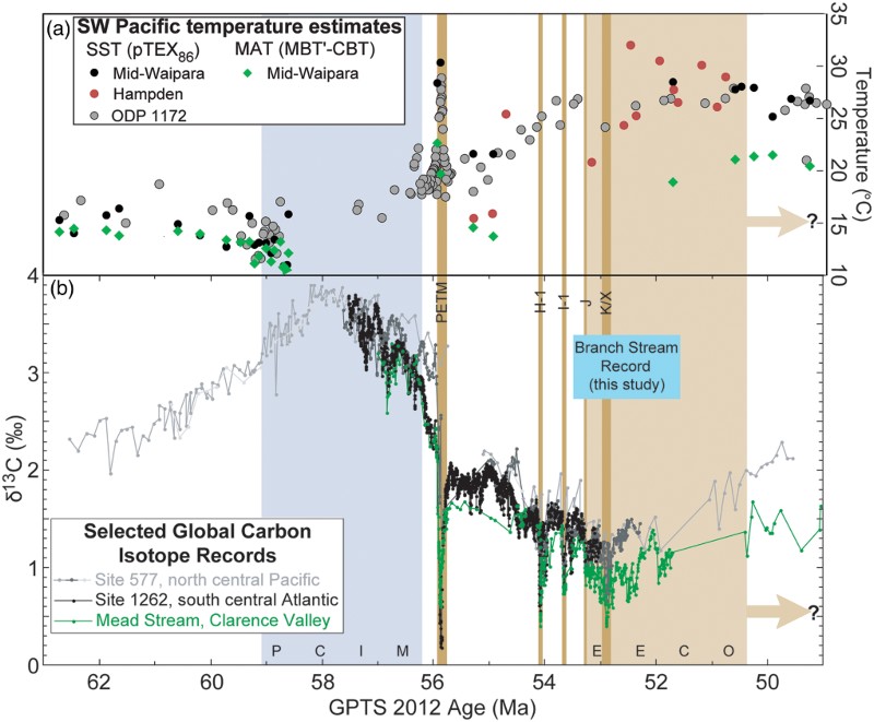
Figure 1 Middle Paleocene to late early Eocene southwest Pacific temperature profiles and global bulk carbonate δ¹³C records. A, Temperature profiles derived from TEX₈₆L and pTEX₈₆ at mid-Waipara and at Site 1172, as well as from Mg/Ca of planktonic and benthic foraminifera at mid-Waipara and Hampden (Burgess et al. 2008; Hollis et al. 2009, 2012; Creech et al. 2010; Sluijs et al. 2011) and from mean air temperature from the MBT’-CBT proxy (Pancost et al. 2013). B, The δ¹³C records are from the central north Pacific (Site 577), central Atlantic (Site 1262) and southwest Pacific (Mead Stream) (Hancock et al. 2003; Nicolo et al. 2007; Zachos et al. 2010; Slotnick et al. 2012; Dickens & Backman 2013). The blue bar denotes the age of the studied section at Branch Stream. Vertical bands mark intervals of major carbon cycle variations: the Paleocene Carbon Isotope Maximum (PCIM; light blue), the EECO (light tan), the PETM and the H-1, I-1 and K/X hyperthermals (dark tan).

To better understand climate and carbon cycling during the EECO, detailed records across the interval are needed from multiple locations, both from widely separated geographic regions and within individual sedimentary basins. Stable carbon isotope stratigraphy provides a powerful means to correlate such records. This is because carbon cycles rapidly (< 2 kyr) between the ocean, atmosphere and biosphere, deviations in climate often relate to variations in net fluxes of organic carbon to and from the exogenic carbon cycle, and organic fluxes have significantly different stable isotope compositions (δ¹³C) than the ocean (Shackleton 1986; Kump & Arthur 1999). Indeed, carbon isotope stratigraphy has already played a prominent role in correlating widely separated early Paleogene sections and in elucidating potential root causes for Earth surface change during this time. This is true for long-term carbon cycle oscillations across the early Paleogene (e.g. Shackleton 1986; Komar et al. 2013), as well as short-term carbon cycle perturbations such as occurred during the PETM (e.g. Koch et al. 1992; Zeebe et al. 2009). Interestingly, however, detailed δ¹³C records across the EECO remain scarce (Fig. 1). This reflects a combination of factors, although the primary reason appears to be a lack of expanded and continuous deep-sea sections, perhaps because of significant calcite compensation depth (CCD) shoaling after the start of the EECO (Leon-Rodriguez & Dickens 2010; Pälike et al. 2012; Komar et al. 2013; Slotnick et al. 2015).

The Clarence River valley, on the northeast of South Island, New Zealand (Fig. 2), is an excellent location to generate detailed early Paleogene δ¹³C records. Several tributaries of the Clarence River expose thick sequences of limestone and marl that originally accumulated as sediment on a passive continental margin from the Late Cretaceous through middle Eocene (Morris 1987; Reay 1993; Strong et al. 1995; Crampton et al. 2003). Initial work suggested that stable carbon isotopes in these sedimentary sequences might faithfully record trends in the δ¹³C of seawater (Nelson & Smith 1996). More recent investigations (Hancock et al. 2003; Hollis et al. 2005a,b; Nicolo et al. 2007; Slotnick et al. 2012) have demonstrated unequivocally that δ¹³C records generated from upper Paleocene and lower Eocene strata in the Clarence River valley can be correlated to δ¹³C records at sites across the world (Fig. 1). From this work two additional findings have emerged (Hollis et al. 2005a,b; Nicolo et al. 2007; Slotnick et al. 2012): (1) prominent negative CIEs generally occur across horizons with higher amounts of clay (marls); and (2) the marls represent enhanced terrigenous accumulation (dilution) rather than reduced carbonate accumulation because of dissolution or reduced productivity. Complementary records and interpretations have arisen from studies focused on the PETM in other continental margin sections (Spain, Schmitz and Pujalte 2003; Italy, Giusberti et al. 2007; USA, John et al. 2008). Collectively, these studies suggest that the hydrological cycle became more intense and more seasonal during intervals of early Paleogene global warmth (Schmitz & Pujalte 2007; Slotnick et al. 2012). In any case, expanded marl-rich sections of Clarence River valley provide a special opportunity to generate detailed δ¹³C records for the EECO (Hollis et al. 2005a; Slotnick et al. 2012).

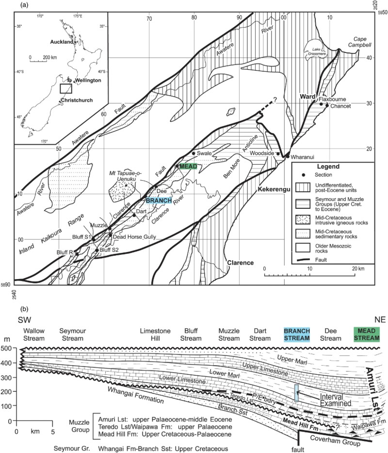
Figure 2 Location and relevant geology of the eastern Marlborough and Kaikoura districts. A, Map showing the general region and outcropping rocks surrounding the Clarence River and adjacent tributary streams (from Crampton et al. 2003). The New Zealand 1:50,000 topographic map P30 (Clarence, NZMS 260) serves as the basis for grid coordinates. Locations of Mead Stream and Branch Stream denoted by blue boxes. B, Schematic cross-section showing relative thicknesses of Muzzle Group rocks found along streams on the north side of Clarence River Valley (adapted from Reay 1993).

Our recent study of the sedimentary sequence at Mead Stream, in the northeast Clarence River valley (Slotnick et al. 2012), provides the most detailed current record of δ¹³C changes through the onset of the EECO. We have identified at least ten negative CIEs, with the most prominent of these equating to the K/X event; that is, a series of CIEs occurred in rapid succession at the onset of the EECO. Initially, this seemed to contrast with δ¹³C records from deep-sea sites (e.g. Sites 577 and 1051; Cramer et al. 2003; Dickens & Backman 2013). However, the δ¹³C signal generated at open ocean locations may not be sufficiently resolved because of much slower sedimentation and core recovery issues (Dickens & Backman 2013).

The objectives of the present study are threefold: (1) to identify and document the EECO interval at a second location in Clarence Valley, namely Branch Stream; (2) to generate a detailed lithologic and δ¹³C record across the EECO and establish the sequence of CIEs, including that which marks the K/X-event; and (3) to compare the new δ¹³C record to those across the EECO at Mead Stream and elsewhere. We selected Branch Stream because the section represents a shallower uppermost slope setting in which land-derived sediments might accumulate at a higher rate than at Mead Stream.

Background

Geological setting

The Clarence River valley trends NE–SW for ∼ 80 km and lies between the Seaward and Inland Kaikoura Ranges in eastern Marlborough, New Zealand (Fig. 2). The Muzzle Group, a lithostratigraphic package of pelagic to hemipelagic Upper Cretaceous to middle Eocene sediments, forms a distinct strike ridge on the northwest side of Clarence River. This sedimentary rock sequence is exposed along several streams that have incised gorges roughly perpendicular to strike. In general, the sequence transitions from a shelf environment in the southwest (e.g. Seymour Stream) to an upper-middle slope environment in the northeast (e.g. Mead Stream), with a paleo-shelf break centred near Muzzle Stream in the middle Clarence River valley (Fig. 2; Reay 1993). Branch Stream is situated approximately midway between Muzzle Stream (∼ 10 km to the southwest) and Mead Stream (∼ 9 km to the northeast).

Sediment deposition of the Muzzle Group occurred along a north-facing embayment of a passive continental margin at ∼ 55–50°S paleolatitude (Crampton et al. 2003; Hollis et al. 2005a). In this setting, variable amounts of biogenic carbonate (principally from calcareous nannofossils), biogenic silica (from diatoms, radiolarians and sponge spicules) and terrigenous clay accumulated on the seafloor (Strong et al. 1995). Most of the biogenic components have since recrystallised to limestone or chert (Lawrence 1989). With the advent of late Cenozoic tectonism throughout New Zealand, beds were subsequently uplifted, folded and faulted so that strata exposed in the Clarence River valley now lie on the northwest limb of a large anticline and dip 40−50° to the northwest (Reay 1993; Rattenbury et al. 2006).

Regional lithostratigraphy

The lithostratigraphic units of interest to this study are the uppermost Lower Limestone and Lower Marl, which comprise the lower portion of the Amuri Limestone Formation (Fig. 2). Names for lithostratigraphic units within the Marlborough region have evolved over time (Morris 1987, pp. 29–37), so clarification is worthwhile. The Upper Cretaceous–Eocene Muzzle Group consists of three formations (Reay 1993; Strong et al. 1995; Hollis et al. 2005a). From oldest to youngest these are: the Mead Hill Formation (Late Cretaceous–early Paleocene), the Waipawa Formation (middle Paleocene) and the Amuri Limestone Formation (late Paleocene–middle Eocene). In turn, the Amuri Limestone Formation in northern Clarence River valley is divided into four lithotypes: the Lower Limestone, the Lower Marl, the Upper Limestone and the Upper Marl. Although these lithotypes are informal units, we follow the practice of our previous papers (e.g. Hollis et al. 2005a,b) and capitalise initial letters to distinguish the units from purely descriptive terms. In order to formalise the units as legitimate members, alternative names will need to be proposed.

Both the Lower Limestone and the Lower Marl consist of decimetre-scale beds of limestone and marl, but the latter lithotype contains more numerous and generally thicker beds of marl (Reay 1993; Hollis et al. 2005a; Nicolo et al. 2007; Slotnick et al. 2012). The limestone beds are very indurated and dominantly composed of low Mg-calcite, whereas the marl beds are not as indurated and contain greater amount of clay minerals, mostly smectite (Lawrence 1989). Beds that are intermediate in character are referred to as marly limestone. Within both units, metre-scale ‘marl-rich intervals’ are identified based on an increase in number and/or thickness of marl beds (Slotnick et al. 2012). Neither uppermost Lower Limestone nor the Lower Marl contain dolomite or appreciable amounts of chert (Lawrence 1989), both of which occur in Mead Hill Formation.

Mead Stream

Beyond studies of Amuri Limestone composition, efforts at Mead Stream have focused on placing this rock formation into a chronostratigraphic framework (Hollis et al. 2005a; Nicolo et al. 2007; Slotnick et al. 2012; Dallanave et al. 2014). At Mead Stream, the Lower Limestone and the Lower Marl are respectively 88 m and 116 m thick, although a 25 m interval of the upper part of the Lower Marl is affected by deformation. The Lower Limestone contains the CIEs associated with the PETM, H-I, H-2, I-1 and I-2 events, while the conformably overlying Lower Marl contains the CIEs associated with the J, K/X and L events. These short-term (<200 kyr) negative CIEs have been identified and labelled from studies of locations around the world (Cramer et al. 2003; Röhl et al. 2005; Agnini et al. 2009; Westerhold et al. 2012). However, at Mead Stream, the Lower Marl has at least eight negative CIEs that have not yet been documented clearly elsewhere (Slotnick et al. 2012).

Branch Stream

Portions of the Muzzle Group are exposed along three tributaries of Branch Stream. Morris (1987) and Reay (1993) described the stratigraphy. Studies have been undertaken on the expanded Cretaceous–Paleogene boundary section (Hollis et al. 2003; Willumsen, 2011), which is well exposed in the middle tributary, but there has been no previous paleoenvironmental study of the Eocene at Branch Stream. The southern and main tributary contains a thick section of Amuri Limestone within a steep gorge. However, the outcrop is more difficult to log and sample than at Mead Stream due to the narrowness of the gorge resulting from fast-flowing water, cascades and a 30 m high waterfall (Fig. 3).

Methods

Stratigraphic log and samples

Above the waterfall, we sampled two sections on the true right side of the gorge that are separated by a major bend in the stream (Fig. 3). The lower of these sections (‘middle section’, named so that a hardier field party might sample rocks across and below the waterfall) consists primarily of bedded limestone with subordinate beds of marl. The upper of these sections (‘upper section’) consists of alternating beds of limestone and marl, transitioning upwards into a marl-dominated succession. The proportion of marl to limestone generally increases up-section. Additional outcrops of the Amuri Limestone lie along a farm track above the stream (Fig. 3) and are generally stratigraphically higher than our ‘upper section’.

We photographed and logged the middle and upper sections (Figs 3 –6). A ‘zero’ datum was set as low in the middle section as possible, just above the waterfall and within the uppermost Lower Limestone. From this datum, strata appear continuous for at least 150 m of stream length, although photographs and samples necessarily jump between the middle and upper sections (Figs 3, 4A, B). The thickness of individual centimetre- to decimetre-scale beds was measured, and beds were identified as one of three lithologies (limestone, marly limestone or marl). A section log was developed by stacking thicknesses of individual beds and then introducing minor scaling to obtain consistent measurements of key horizons compared to a tape and compass traverse (Fig. 6). Correlations between the middle and upper sections were inferred by eye in the field and subsequently constrained by matching carbon isotope records (Fig. 5B). Detailed photographic logs of the sections, with sample positions indicated, are available.

Figure 3 Location of the logged sections at Branch Stream, including the nearby farm track section. A, Part of Topo50 sheet BS27 (Tapuae-O-Uenuku) showing the main gorge (contour interval – 20m). B, Schematic illustration showing the two sections (middle and upper) within the gorge, as well as strike and dip indicators and the position of the K/X event, which is found in both sections. Light blue and green ‘cameras’ represent location and orientation of photographs in Figures 4 and 5.

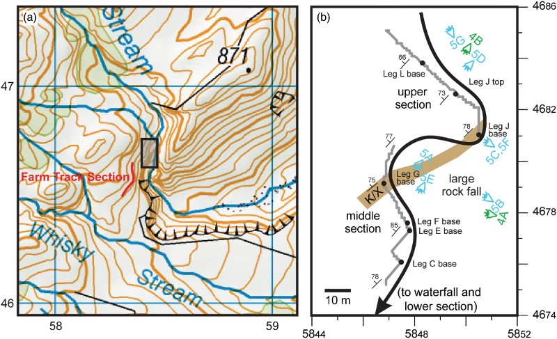
Figure 4 Photographs showing the two sections at Branch Stream, with downstream indicated by blue arrows. Selected samples taken for geochemistry and paleomagnetism are presented for reference with white lines and labels. A, Middle section with the basal ‘zero’ datum near the far left, and the position of the J and K/X events shown by tan bands. B, Most of the upper section with the L event shown by a tan band. For both panels, scale bars are approximate to the centre of the field of view.

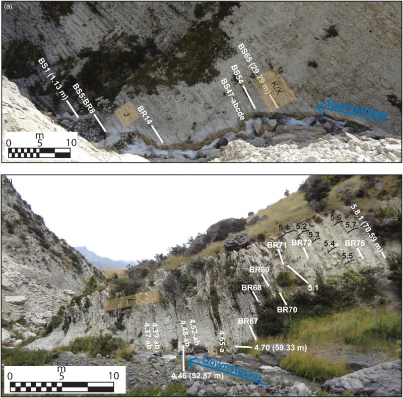
Figure 5 Photographs highlight specific features at Branch Stream, with downstream direction indicated by blue arrows. A, Middle section between the J and K/X events. B, Downwards view of the tie point between the middle and upper sections. C, Horizontal image of the K/X event at base of the upper section. D, An interval of mostly limestone with recessed marl horizons just above the L event in the upper section. E, Image looking down the gorge with ‘zero’ datum marked in black. Note that the main gorge continues below the ‘zero’ datum, but there exists a major waterfall. F, Detailed image of K/X event where δ¹³C reaches a minimum (Fig. 6). G, Image looking up the gorge at Mount Tapuae-O-Uenuku framed by Upper Limestone, which lies above the logged section. For photographs B, E and G, approximate scales are placed on convenient exposures with acknowledgement that the field of view and scale changes significantly.

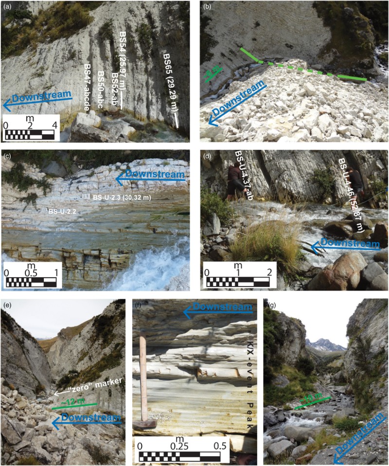
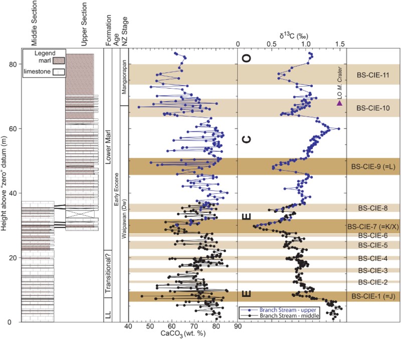
Figure 6 The lower–middle Eocene composite section at Branch Stream comprising two overlapping sections, and records of carbonate content and bulk carbonate δ¹³C. The boundary between the Lower Limestone and Lower Marl members of the Amuri Limestone (after Reay 1993) is gradational over 17 m. The Waipawan/Mangaorapan Boundary is placed at the lowest occurrence of Morozovella crater (Table S2). Dark tan bands represent carbon isotope excursions (CIEs) identified in deep-sea records; light tan bands represent CIEs identified at Branch or Mead streams. Labelling of the CIEs follows that shown in Table S1 and Table 1.

A total of 351 fresh rock samples were collected from the two sections for geochemical and biostratigraphic analysis (Fig. 5D). Samples were labelled on the outcrop and subsequently given GNS Science curation numbers and New Zealand Fossil Record numbers (Table S1). Because samples were collected by hammer and chisel they vary in size and shape, but generally exceeded 300 g in weight. Samples were taken to ensure stratigraphic overlap between the middle and upper sections. Sampling resolution of ∼ 22 cm is similar to that of the corresponding interval at Mead Stream (Slotnick et al. 2012, 2014).

Samples were collected for the study of calcareous nannofossils, radiolarians and foraminifera. However, we only report on the foraminiferal biostratigraphy here. Foraminifera are generally not well preserved in the Amuri Limestone Formation and are not easily extracted from limestone or marly limestone beds; however, identifiable specimens can be found in the marl beds (Strong et al. 1995; Hancock et al. 2003). A total of 32 marl beds or thin marl interbeds were selected for foraminiferal study.

Sample preparation and analyses

After samples were bagged in the field and their location marked, they were carried out on foot and transported to a rock preparation lab. Weathering rinds were removed with a rock saw. Aliquots of marl samples were taken for microfossil examination, and aliquots of most samples were taken for geochemical analysis. These were freeze-dried to remove potential water and powdered in a tungsten carbide rock mill. Powdered samples were then analysed for carbonate content and stable isotope composition. Sufficient bulk sample was retained for further paleontological and geochemical studies.

The carbonate bomb method (Dunn 1980) was used to determine carbonate content (Table S1). A ±1.3% analytical precision (1σ) was determined from calibration curves and from multiple analyses of an in-house standard. Bulk stable isotopes were measured at the Stable Isotope Lab, GNS Science, Lower Hutt. Analyses were completed on a GVI IsoPrime Carbonate Preparation System at a reaction temperature of 25 °C for 24 hours and run via dual inlet on the IsoPrime mass spectrometer. All results are reported in conventional delta notation with respect to Vienna PeeDee belemnite (VPDB) via integration to the NBS-18 and NBS-19 standards and normalisation to Carrera Marble, an internal standard with reported values of 2.04‰ for δ¹³C and –6.40‰ for δ¹⁸O (Table S1). The precision of our stable isotope measurements is better than 0.1‰ for δ¹³C and better than 0.2‰ for δ¹⁸O.

Selected marl samples were processed at GNS Science for their foraminifera assemblages using a washing procedure. Samples were dried, crushed and soaked in warm water and calgon for at least 12 hours. Samples were then washed through a 75 μm screen and oven dried at 40 °C. Dried residues were sieved into >500 μm, >150 μm and pan fractions. Depending on the amounts of material, most of the >500 μm fraction and a small portion of the pan fraction were examined for foraminifera. The >150 μm fraction was subdivided using a riffle splitter to yield one well-strewn picking tray, containing several hundred specimens for most samples. Approximate percentages of agglutinated benthic, calcareous benthic and planktic foraminifera were determined from 100 specimens using a laboratory counter along random traverses. For poorly fossiliferous samples, all specimens were extracted and percentages derived from the total number obtained. After counting, representative specimens of all taxa were extracted and key foraminifera taxa, both benthic and planktic, were identified but were not counted individually. Other specimens were identified to genus level and placed in open nomenclature.

Results

Lithology and bedding

The total stratigraphic thickness of the composite of the middle and upper sections is 84 m. The sequence represents a thick, near-continuous calcareous-rich package of the uppermost Lower Limestone and most of the Lower Marl.

The transition from the Lower Limestone to the Lower Marl is not as well defined at Branch Stream as it is at Mead Stream (Figs 5A, 6). Instead, the transition occurs gradually between 5.3 and 21.8 m. Recessed beds of marl increase in frequency across this interval, comprising 8% of the succession from 0.0 to 5.3 m, 15% from 5.3 to 21.8 m and 48% of the succession from 21.8 to 83.4 m.

The uppermost Lower Limestone (0.0–5.3 m) consists mainly of centimetre- to decimetre-scale beds of hard, grey limestone (Fig. 6). Two relatively marl-rich horizons crop out between 2.5 and 2.7 m and between 3.5 and 3.7 m. Across the transition to the Lower Marl, marl partings or thin (<10 cm) marl beds separate limestone beds, including distinct intervals consisting of more numerous individual marl beds from 7.39 to 9.49 m, 12.37 to 12.74 m, 15.21 to 16.19 m and 19.51 to 20.02 m (Table 1).

Table 1 Carbon isotope excursions (CIE) at Branch and Mead streams.

Branch Stream CIE	Magnitude of CIE, Branch (δ13C ‰)	Height of CIE minimum, Branch (m)	Magnitude of CIE, Mead (δ13C ‰)	Height of CIE minimum Mead (m)	Nomenclature at other locations
BS-CIE-11	0.5	75.64	0.4	266.60
BS-CIE-10	0.5	64.45	0.4	256.60
			0.3	241.46	L2
BS-CIE-9	0.5	47.62	0.4	236.52	L
BS-CIE-8	0.4	34.82	0.4	226.86
BS-CIE-7	0.6	29.87	0.5	222.35	K / X / ETM-3
BS-CIE-6	0.3	26.94	0.3	219.92
BS-CIE-5	0.3	23.45	0.3	217.97
BS-CIE-4	0.3	19.69	0.2	213.88
BS-CIE-3	0.1	16.54	0.1	212.74
BS-CIE-2	0.2	12.54	0.2	210.14
BS-CIE-1	0.6	8.54	0.4	207.31	J

This list serves as a way to maintain clarity between each CIE and/or hyperthermal expressed lithologically and chemically at Branch Stream.

The Lower Marl (sensu stricto) begins at 21.8 m and continues for the remainder of the logged section (Fig. 6). The unit includes numerous and thick recessed marl beds alternating with limestone and marly limestone beds, and includes distinct intervals with more numerous marl beds such as between 27.95 and 31.09 m. Marl layers account for ∼ 50% of the succession from 21.8 to 30.2 m, ∼ 25% of exposed outcrop from 30.2 to 63.8 m and ∼ 88% of the succession from 63.8 to 83.4 m. The only noticeable internal deformation within the Lower Marl at Branch Stream is an interval of boudinage from 48.5 to 49.0 m. Rock scree also covers ∼ 3 m of section near the base of the upper section, although this interval can be documented and sampled in the upper part of the middle section. Most of the Lower Marl is better exposed at Branch Stream than at Mead Stream; the latter had a few intervals that could not be sampled closely (at least between 1995 and 2014) because of vegetation or rock scree (Nicolo et al. 2007; Slotnick et al. 2012). However, the upper interval of Lower Marl, while present at Mead Stream, is either partially covered by rock scree or absent from Branch Stream. In any case, the top of the Lower Marl lies above our ‘upper section’ at Branch Stream.

Carbonate content

Although variable, the carbonate content shows distinct trends (Fig. 6). Across all samples, it averages 72 ± 8% (1σ) and ranges from 45 to 85%. Partitioned by lithology, the means and standard deviations for CaCO₃ content are (at 1σ) 61 ± 5% (n = 102), 71 ± 4% (n = 58) and 77 ± 4% (n = 226) for marl, marly limestone and limestone, respectively. Carbonate content is generally lower across four specific intervals: it averages 65 ± 7% for 10.6–17.4 m, 27.5–31.8 m, 45.8–48.0 m and 64.0–83.4 m.

Carbon isotopes

Bulk carbonate δ¹³C analyses yield a curve with obvious trends and CIEs (Fig. 6). Overall, values range between 1.52 and 0.24‰ with an average of 0.93 ± 0.23‰ at 1σ. The most enriched values (1.23–1.52‰) span two intervals: the basal part at 0–7.2 m and at 58.0–61.4 m. The most depleted values (<1.00‰) span three intervals: 8.1–51.0 m, 63.7–66.6 m and 73.6–80.0 m. Eleven CIEs in total, defined here as ‘marked decreases in δ¹³C expressed by numerous (>5) successive samples across narrow (<5 m) stratigraphic intervals’, are identified in the composite section (Tables 1, 2). We refer to these as Branch Stream carbon isotope excursions (i.e. BS-CIE-n, where n is 1–11). The lowest δ¹³C value of the dataset (0.24‰) represents the minimum of BS-CIE-7, and is found at 29.87 m. The magnitudes of all 11 CIEs range from 0.1 to 0.6‰, values that are far greater than analytical precision.

The CIEs identified at Branch Stream generally coincide with ‘marl-rich intervals’, where the number and thickness of recessed marl beds increases. Importantly, though, the correspondence is not exact at the centimetre- to decimetre-scale (Fig. 6). This is because, at the small scale, the δ¹³C composition of a particular sample does not relate directly to rock type, carbonate content or recessed patterns. For example, BS-CIE-1 and BS-CIE-9 span multiple beds of marl and limestone (Fig. 7). As a consequence, there is no obvious relationship between carbonate content and δ¹³C across the sample suite (Fig. 8), an observation that also has been made for the Amuri Limestone at Mead Stream (Slotnick et al. 2012).

Figure 7 Lithologic, carbonate content and stable carbon isotope records across two short CIEs within the transition from Lower Limestone to Lower Marl or in Lower Marl: A, the J event; and B, the L event.

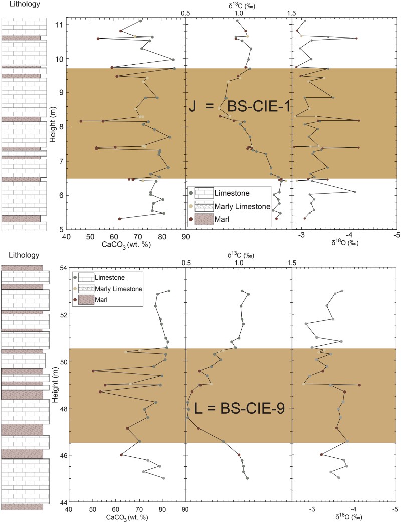
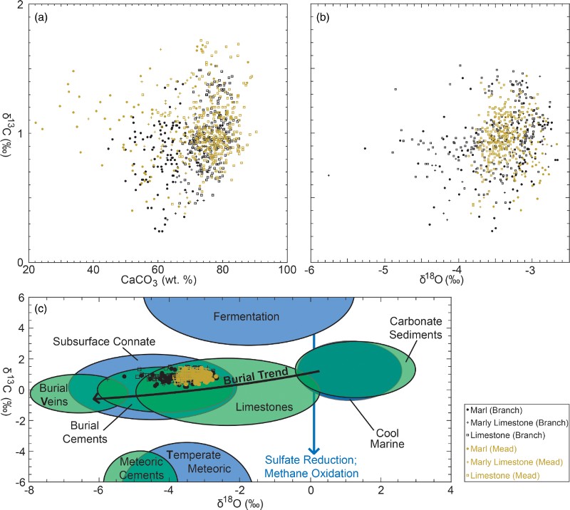
Figure 8 Bulk carbonate content and stable isotope compositions for all Lower Eocene samples examined to date at Branch and Mead streams plotted according to lithology. Note that there is no obvious relationship between δ¹³C and carbonate content, despite the clear signal in δ¹³C over time (Fig. 6). Note also the significant depletion in ¹⁸O relative to typical carbonate in unlithified marine sediment. The stable isotope compositions are consistent with significant local dissolution and reprecipitation of carbonate during burial. Fields of carbonate stable isotope composition are from Hudson (1977) and Nelson and Campbell (1996).

Foraminifera

Most marl samples examined for foraminifera contain identifiable specimens of both planktic and benthic foraminifera, with the latter usually less than 20% of the total assemblage (Table S2). Biostratigraphic assessment of the faunal assemblages indicates that the gorge sections can be correlated loosely to the early Eocene planktonic foraminiferal biozones E4–E6 (Berggren & Pearson 2005). This is because samples from 48.69 m to 78.85 m at Branch Stream contain Morozovella lensiformis, which is a common component of foraminifera assemblages representing upper foraminiferal biozone E4 and lower foraminiferal biozone E5. At low-latitude locations, the range of M. lensiformis extends from 54.6 Ma to 53.1 Ma (Gradstein et al. 2012). Foraminiferal assemblages also contain benthic taxa (e.g. Glomospira, Ammodiscus, Vulvulina, Nuttallides, Pleurostomella and Stilostomella), indicative of deposition in middle bathyal (600–1000 m) to lower middle bathyal (800–1000 m) or possibly deeper environments.

Planktic foraminifera datums in Paleogene strata of New Zealand cannot be tied precisely to biozonation schemes that have been developed elsewhere; key taxa used in low- or high-latitude schemes appear at different times in New Zealand or are simply not present (Hornibrook et al. 1989; Hancock et al. 2003). The long-term isolation of New Zealand in middle Southern Hemisphere latitudes underpins the rationale for a robust regional New Zealand Geological Time Scale (Cooper 2004; Raine et al. 2015).

Several key foraminifera markers were identified at Branch Stream (Table S2). First, the lowest occurrence of Pseudohasterigina wilcoxensis was found at 8.18 m. This datum has been used to distinguish an upper portion of the New Zealand Waipawan Stage (Cooper 2004). From work at Dee Stream, this datum occurred well after the PETM and ETM-2/H-1 events (Hancock et al. 2003), the latter of which is dated at ∼ 54.1 Ma (GTS2012, Gradstein et al. 2012). The second foraminifera marker is the presence of Morozovella acuta and M. aequa at 0.0–28.25 m. The third is the presence of M. aequa but absence of M. acuta at 28.25–34.93 m. The fourth marker is the lowest occurrence of Morozovella lensiformis at 45.97 m. The fifth foraminifera marker is the lowest occurrence of Morozovella crater, which defines the base of the New Zealand Mangaorapan Stage, at 67.00 m (Fig. 6). Following recent recalibration of the New Zealand Geological Time Scale to GTS2012 (Raine et al. 2015), this datum has a revised age of 52.0 Ma. This age is based on integrated magnetostratigraphy and calcareous nannofossil biostratigraphy at Mead Stream (Dallanave et al. 2014), where the lowest occurrence of M. crater occurs in uppermost Chron C23r (Raine et al. 2015). Finally, the sixth marker is the highest occurrence of the agglutinated benthic foraminifera Gaudryina reliqua at 74.89 m. The HO of Gaudryina reliqua has been tentatively proposed as a proxy for the Mangaorapan-Hertaungan stage boundary where the Heretaungan index, Elphidium hampdenense, is not present. In summary, foraminiferal biostratigraphy indicates that the measured section was deposited during the late Waipawan (Dw) and Mangaorapan (Dm), and possibly the early Heretaungan (Dh) stages, implying a maximum age range of 54–48 Ma.

Discussion

The age of the Early Eocene Climatic Optimum

The term EECO first came to widespread attention when Zachos et al. (2001) showed that a composite benthic foraminifera stable isotope record displayed a broad 2–3 Myr long minimum in δ¹⁸O within the middle–latest early Eocene. This minimum in δ¹⁸O generally correlated with evidence for very warm climates observed at several locations (e.g. West & Dawson 1978; Wing et al. 1991; Dingle & Lavelle 1998) and was therefore called the ‘Early Eocene Climatic Optimum’ (Zachos et al. 2001). The EECO was initially inferred to span a time interval from about 52 to 50 Ma, but the event itself was not formally defined. Moreover, the absolute ages came from an age model (Berggren et al. 1995) that is now out of date (Westerhold & Röhl 2009; Gradstein et al. 2012; Westerhold et al. 2012).

The absolute age and duration of the EECO remain problematic for two reasons. First, there are relatively few locations where good records of past temperature can be clearly linked to a geopolarity time scale. Second, a given temperature threshold or warming trend may have occurred at different times, depending on location, especially when considering modern temperature variability across the globe. Defining the start and end of a multi-million-year interval of extreme Cenozoic global warmth on the basis of temperature, and using temperature as a means of correlation between widespread sites, is an inherently challenging exercise.

The benthic foraminifera δ¹⁸O measurements originally used to ‘define’ the EECO were accompanied by δ¹³C measurements. This is important because, unlike δ¹⁸O and temperature measurements, it is very clear that (at least in certain rock sequences) early Paleogene records from widespread locations can be correlated at fine temporal resolution using carbon isotope stratigraphy (Zachos et al. 2010; Slotnick et al. 2012; Littler et al. 2014). The beginning of the EECO, at least as presented by Zachos et al. (2001), happened at or just before a pronounced low in δ¹³C. This low can be shown to mark the K/X event (Dickens & Backman 2013), which occurred 3.0 ± 0.2 Myr after the PETM (Westerhold et al. 2012). On the current GPTS 2012 time scale (Gradstein et al. 2012), the PETM and K/X events are dated at 55.9 and 52.9 Ma, respectively (Westerhold et al. 2009; Hilgen et al. 2010; Charles et al. 2011; Vandenberghe et al. 2012) (Fig. 1, Table 2).

Table 2 Early Eocene carbon isotopic tie points for Mead and Branch streams.

Datum	Branch height (m)	Mead height (m)	Age (Ma)
	75.64	266.60	51.84
BS-CIE-10 – base	64.45	256.00	52.11
	60.03	252.22	52.19
BS-CIE-7 (K/X) – top	31.80	225.35	52.83
BS-CIE-7 (K/X)	30.32	223.15	52.88
BS-CIE-7 (K/X) – peak	29.87	222.35	52.90
BS-CIE-7 (K/X)	28.81	221.84	52.91
BS-CIE-7 (K/X) – base	27.66	220.90	52.93
BS-CIE-5 – top	24.87	217.95	52.98
BS-CIE-5 – base	22.21	216.09	53.01
BS-CIE-4	19.51	213.80	53.07
BS-CIE-3 – top	16.82	212.78	53.09
BS-CIE-1 (J)	8.18	206.70	53.25

In the southwest Pacific region, there is evidence for warmer conditions beginning at 54–52 Ma (Fig. 1). This includes estimates for sea-surface temperature derived from the TEX₈₆ proxy and Mg/Ca ratios (Bijl et al. 2009; Hollis et al. 2009, 2012) and mean air temperature from the methylation index of branched tetraethers (MBT)’-cyclization index of branched tetraethers (CBT) proxy (Pancost et al. 2013). Although records are patchy during the onset of this warming interval, there is general agreement between sites and proxies that peak temperatures occurred at 52–49 Ma. This broadly corresponds to the Mangaorapan Stage (Raine et al. 2015), which has previously been identified as having the warmest conditions in New Zealand during the Cenozoic (Hornibrook 1992). At Mead Stream, the K/X event occurs just above the bottom of the Lower Marl (Slotnick et al. 2012), whereas the base of the Mangaorapan is close to the start of a marl-dominated facies within Lower Marl (Dallanave et al. 2014).

Stratigraphy at Branch Stream

With this knowledge of the likely timing of the onset of the EECO and its relationships with early Eocene CIEs, we can interpret the Branch Stream section as follows.

Both the lithology and carbon isotope data at Branch Stream can be used to splice the middle and upper sections together (Fig. 6). That is, the two studied sections (Fig. 4) overlap to make an apparently complete composite section because the major bend in the stream cuts back across-strike and down-section (Fig. 3).

The composite section can be correlated to Mead Stream. Bulk carbonate δ¹³C trends from the uppermost Lower Limestone and the Lower Marl are very similar at Branch and Mead streams (Fig. 9). At both sites, there is an overall 1.2‰ drop in δ¹³C and a subsequent 1.2‰ rise in δ¹³C across the transition from the Lower Limestone to the Lower Marl. At both locations, there is a ‘step-like’ 0.5‰ CIE (BS-CIE-1) at the start of this transition. At both sites, there is a prominent 0.5‰ CIE (BS-CIE-7) about 25–30 m above this transition, which marks the lowest δ¹³C value. The magnitudes and relative positions of minor CIEs are also very similar (Table 1). The one significant difference is that BS-CIE-9 appears as two successive CIEs at Mead Stream (Fig. 9).

Figure 9 Records of carbonate content and bulk carbonate δ¹³C at Branch and Mead streams plotted against stratigraphic height at both locations. For Mead Stream, formation names, lithology and biostratigraphy are derived from Hollis et al. (2005a), with minor adjustments (Slotnick et al. 2012). Carbonate content and δ¹³C data for Mead Steam are from Slotnick et al. (2012) with some additional samples (Slotnick et al. 2014). Paleomagnetic data come from Dallanave et al. (2014). Dark tan intervals represent prominent CIEs found in deep-sea records, whereas light tan intervals represent additional CIEs identified at Branch and Mead streams. Because Mead Stream has a well-refined stratigraphy now grounded with polarity chrons, profile and tie points using distinct changes in δ¹³C can be used to establish an age model at Branch Stream (Table 2).

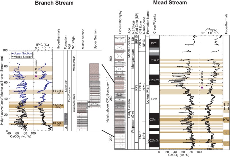
Much of the Lower Limestone and most of the Lower Marl at Mead Stream has been correlated to sections in deep-sea locations through biostratigraphy, carbon isotope stratigraphy and magnetostratigraphy (Hollis et al. 2005a; Nicolo et al. 2007; Slotnick et al. 2012; Dallanave et al. 2014). This has been carried out as follows. First, available foraminifera, radiolarian and nannofossil datums (Strong et al. 1995; Hollis et al. 2005a) were compared to those at other locations, including at Sites 577 and 1262 (Zachos et al. 2004; Agnini et al. 2007; Dickens & Backman 2013). Second, a ‘high-resolution’ δ¹³C record was generated at Mead Stream within this biostratigraphic framework and aligned to comparable records at sites drilled in the deep sea, particularly DSDP Site 577 and ODP Site 1262. The assumption here is that a specific sequence of early Paleogene CIEs exists, and these represent past changes in carbon fluxes to and from the combined ocean–atmosphere carbon reservoir (Shackleton et al. 1985; Cramer et al. 2003; Zachos et al. 2010). Third, where δ¹³C records remain poorly defined at deep-sea sites, CIEs at Mead Stream were linked to magnetic susceptibility (MS) peaks at Site 1262. The assumption here is that the MS peaks at Site 1262 represent times of deep-sea carbonate dissolution relating to past changes in global carbon fluxes and hence CIEs (Lourens et al. 2005; Nicolo et al. 2007; Zachos et al. 2010). Fourth, a polarity chron record was determined at Mead Stream (Dallanave et al. 2014). This is a powerful verification of any stratigraphic interpretation (Fig. 9). Notably, the ‘step-like’ BS-CIE-1 occurs within polarity subchron C24n.2r (53.42–53.27 Ma) and must equate to the J event, which occurred at 53.35 Ma, and the prominent BS-CIE-7 occurs within polarity subchron C24n.1n (53.07–52.62 Ma) and must equate to the K/X event, which occurred at 52.9 Ma.

The foraminiferal assemblages support a late early Eocene age for the Branch Stream composite section. However, they also emphasise an issue regarding the base of the Mangaorapan Stage (Raine et al. 2015). Previous low-resolution stratigraphic studies in New Zealand indicated that primary datum for the base of the stage, lowest occurrence of M. crater, coincided with a well-dated nannofossil event, lowest occurrence of Discoaster lodoensis. This proxy datum has served as the basis for the age of the base of the Mangaorapan Stage for several years (Cooper 2004; Hollis et al. 2010). However, the recent integrated magnetostratigraphic and biostratigraphic study of Mead Stream section (Dallanave et al. 2014) shows that these two events are offset by 40 m with the lowest occurrence of M. crater occurring in uppermost Chron C23r, resulting in a revised age for the base of the Mangaorapan of 52 Ma. This age is consistent with the Branch Stream record where the lowest occurrence of M. crater occurs and where section becomes marl-dominant ∼ 40 m above the K/X event (Fig. 6).

Through the above stratigraphic correlations, the measured composite section at Branch Stream was deposited during 53.4–51.6 Ma. Furthermore, the 11 CIEs can be given approximate ages (Table 2). Significantly, the five most prominent CIEs (BS-CIE-1, 7, 9, 10 and 11) are approximately 400 kyr apart, which lends weight to the hypothesis that major CIEs of the early Paleogene are related to changes in the eccentricity of Earth's orbit (Lourens et al. 2005; Nicolo et al. 2007; Westerhold & Röhl 2009; Zachos et al. 2010; Littler et al. 2014).

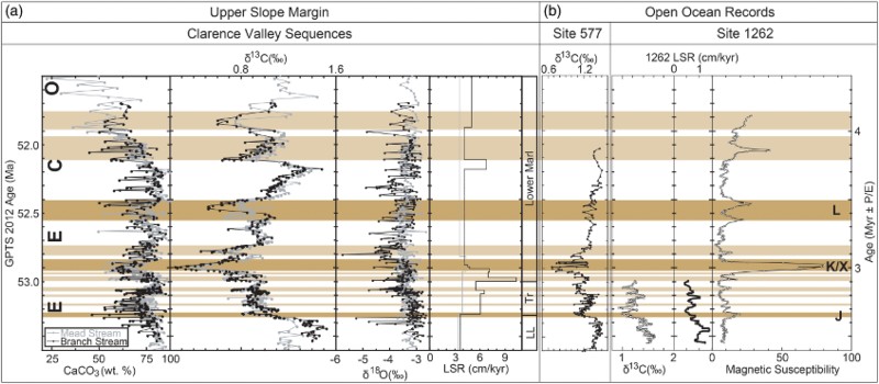
Whether 11 CIEs span the 53.4–51.6 Ma time interval at localities outside of the Clarence River valley is not yet clear. Certainly, the J, K/X and L events have been documented at numerous sites (Cramer et al. 2003; Agnini et al. 2009; Coccioni et al. 2012). However, some of the smaller CIEs found at Branch Stream and Mead Stream have not been highlighted elsewhere, although they may exist without designation (Fig. 10). For example, the modest CIEs preceding and closely following K/X (BS-CIE-4 and BS-CIE-8) may exist at DSDP Site 577 (Cramer et al. 2003). Perhaps most convincing is the MS record at ODP Site 1262 (Fig. 10). At this deep-sea location, the J and K/X events (as well as the PETM and H1/ETM-2 events) are marked by CIEs as well as carbonate dissolution horizons, the latter of which manifest as highs in MS. It appears that each CIE found at Branch and Mead streams corresponds to a high in MS at Site 1262, and with somewhat similar magnitude. Altogether, we suspect there is a very specific series of CIEs that have generally been overlooked in deep-sea sediment cores due to low sampling resolution and their condensed nature. Moreover, this sequence of CIEs broadly marks the start of EECO, at least as defined from benthic foraminifera stable isotope records (Zachos et al. 2001).

Figure 10 Records from the Clarence Valley sections compared to selected locations elsewhere: A, Carbonate content, bulk carbonate δ¹³C and δ¹⁸O and linear sedimentation rates at Branch and Mead streams; and B, Bulk carbonate δ¹³C, linear sedimentation rates and magnetic susceptibility at Sites 577 (central north Pacific) and 1262 (central south Atlantic) (Cramer et al. 2003; Zachos et al. 2004; Zachos et al. 2010; Slotnick et al. 2012; Dickens & Backman 2013).

Marl-rich units and increased terrestrial discharge during the EECO

At Mead Stream, marl-rich intervals within the Amuri Limestone have higher compacted sedimentation rates than surrounding limestone-rich intervals (Hollis et al. 2005a; Nicolo et al. 2007; Slotnick et al. 2012; Dallanave et al. 2014). This is true at the large scale and at the small scale. For example, the Lower Limestone, which includes expanded horizons across the PETM, H and I events, has an average compacted sedimentation rate of ∼ 1.8 cm/kyr; in contrast, the Lower Marl across the start of EECO (204–314 m) has an average compacted sedimentation rate of ∼ 2.6 cm/kyr (Slotnick et al. 2012, 2014).

The marl-rich intervals at Branch Stream also appear to represent periods of higher sedimentation rates. The 84 m composite section was deposited over ∼ 1.8 Myr, giving an average compacted sedimentation rate of ∼ 4.7 cm/kyr. However, the relatively marl-rich interval between BS-CIE-1 (J event) and BS-CIE-7 (K/X event) was ∼ 21.3 m, whereas the relatively limestone-rich intervals between BS-CIE-7 and BS-CIE-9 and between BS-CIE-9 and BS-CIE-10 was 17.8 m and 16.8 m, respectively (Fig. 6). Should the time between these CIEs consistently represent ∼ 400 kyr, the compacted sedimentation rate was ∼ 5.3 cm/kyr across the first interval but only ∼ 4.4 and ∼ 4.2 cm/kyr across the latter intervals.

Irrespective of detailed sedimentation rates, which would require more refined age dates for each CIE, the Lower Marl at both Mead Stream and Branch Stream appears to be a lithological expression of EECO, where elevated global temperatures relate to a greater abundance of siliciclastic sediment on the ancient New Zealand margin. A comparison of the two sections offers insight to the cause. The ∼ 84 m composite section at Branch Stream correlates to a ∼ 65 m interval at Mead Stream (Fig. 9), about a 23% reduction in sedimentary thickness to the northeast. The CIEs at Mead Stream also appear thinner. For example, BS-CIE-1 (J event) spans 3.1 m at Branch Stream but only 1.2 m at Mead Stream; BS-CIE-7 (the K/X event) spans 4.0 m at Branch Stream, but only 3.6 m at Mead Stream. Furthermore, the average carbonate contents are slightly lower at Branch Stream (71.7 ± 8.0%; n = 351) than at Mead Stream (73.5 ± 9.1%; n = 337). A simple explanation for these observations is that, during the Paleogene, Branch Stream was slightly closer to the ancient coastline and received more terrigenous sediment during times of elevated warmth.

The idea of enhanced siliciclastic delivery to continental margins during past intervals of warmth is consistent with model-based climate projections and historic river discharge data. Elevated Earth surface temperatures should lead to greater amounts of rain on land at many locations, but over a shorter portion of the year (Peterson et al. 2002; Murphy et al. 2004; Held & Soden 2006; Meehl et al. 2007a,b). Such precipitation should intensify erosion, so that greater fluxes of terrigenous material debouch onto the continental slope (Ludwig & Probst 1998; Schmitz & Pujalte 2003, 2007). Certainly, terrigenous sedimentation rates increased across the PETM at several continental margin locations (Schmitz & Pujalte 2003; Giusberti et al. 2007; John et al. 2008).

Interestingly, there are subtle differences in the δ¹³C records at Branch and Mead streams. Branch Stream has a wider range of carbon isotope values (0.24–1.52‰) compared to Mead Stream (0.38–1.44‰) and a greater magnitude for several CIEs, including the K/X event (Table 1; Fig. 10). As now evident for the PETM and H-1 events, the magnitude of a particular CIE can vary significantly from one location to another (McInerney & Wing 2011; Sluijs & Dickens 2012). This arises for three main reasons: the mixing of similar components with different isotopic composition; variable changes in fractionation among different components; and local variations in the environment (Sluijs & Dickens 2012). We cannot rigorously argue for any particular process without further analysis. Nonetheless, the differences appear real and probably reflect local factors. One possibility is that greater riverine discharge during short-term warming events decreased the δ¹³C of dissolved inorganic carbon (DIC) of surface water along the margin, but this effect was more pronounced with proximity to the coast (Dickens 2011). A δ¹³C gradient can occur across modern margins because riverine DIC generally has a much lower δ¹³C than that of seawater (Spiker & Schemel 1979; Chanton & Lewis 1999). Rivers can also discharge dissolved organic carbon (DOC) which has a much lower δ¹³C than seawater (Peterson et al. 1994; Hedges et al. 1997), and some of this might convert to DIC relatively quickly (Vodacek et al. 1997). Another possibility is differential diagenesis.

Differential diagenesis and stable isotopes

The formation of marine rock sequences comprising alternating beds of limestone and marl has been discussed extensively (Hallam 1964, 1986; Ricken 1996; Westphal et al. 2010). Gradational boundaries typically separate calcareous-rich and clay-rich intervals in shallowly buried (<200–300 m) marine sediment along modern continental margins. The sharp boundaries commonly observed in the rock record therefore strongly suggest an important diagenetic role. Outcrop proof for such diagenesis includes beds passing laterally into concretions and beds thickening or thinning relative to one another.

A general process called ‘differential diagenesis’ explains limestone and marl couplets in numerous rock sequences (Eder 1982; Ricken 1986; Frank et al. 1999; Westphal et al. 2010). During sediment burial, and at a modest depth below the seafloor, carbonate transfer occurs from strongly compacting clay-rich intervals to minimally compacting calcareous-rich intervals on the decimetre-scale because of pressure solution (Matter et al. 1975; Arthur et al. 1984). This mechanism explains the enhanced bedding, as well as a range of microscopic observations such as carbonate overgrowth on microscopic tests and recrystallisation in limestone beds. Importantly, differential diagenesis also impacts the chemistry including stable isotopes (Matter et al. 1975; Hudson 1977; Frank et al. 1999; Westphal et al. 2010). In general, the δ¹³C of carbonate should be minimally affected; however, the δ¹⁸O of carbonate should be strongly affected. This occurs for three reasons (above references and Scholle & Arthur 1980): (1) there is a considerable volume of pore water in shallowly buried marine sediment (typically >60% within the upper few hundred metres); (2) there are major differences in the amounts of carbon and oxygen hosted in water and sediment, respectively; and (3) there is a much greater influence of temperature upon oxygen isotope fractionation during carbonate precipitation compared to carbon isotope fractionation.

Most of the Amuri Limestone has likely experienced ‘differential diagenesis’ (Lawrence 1989). Beyond the mostly sharp contacts separating limestone and marl beds, and thinning and thickening of individual beds, there are notable differences between the different beds in terms of elemental chemistry and the preservation of calcareous microfossils. In particular, the marl beds contain extractable, identifiable foraminifera with signs of dissolution, whereas the limestone beds have common calcareous nannofossils with carbonate overgrowths (Lawrence 1989). It is therefore interesting to consider the extent to which our stable isotope dataset at Branch Stream reflects diagenetic modification of initial sediment composition.

Stable carbon isotopes at Branch Stream are consistent with differential diagenesis, albeit with an interesting implication. As emphasised above, variations in the δ¹³C record are not linked to lithology at the decimetre-scale (Fig. 7) but are correlative in the time domain to δ¹³C variations elsewhere (Fig. 10). This combination of observations suggests that carbonate diagenesis occurred within a closed system at the local scale, where almost all carbon mass in a volume of sediment existed as carbonate before limestone formation; otherwise, the striking δ¹³C signal, which can be correlated to similar records regionally and globally, would have been erased. However, when it is realised that local transfer of CO₃^2– likely occurred from clay-rich horizons to carbonate-rich horizons (Arthur et al. 1984; Frank et al. 1999), and that clay-rich horizons probably correspond to hyperthermal events characterised by lows in the δ¹³C of the exogenic carbon cycle, a necessary implication is that the CIEs in the Amuri Limestone should generally be muted relative to correlative CIEs found in other locations without diagenetic overprinting. This is because carbonate in the marls, which started with relatively low δ¹³C, has been shuttled to neighbouring limestone beds, which started with relatively high δ¹³C. This appears to be the case, as correlative bulk carbonate CIEs seem to have slightly smaller amplitude at Mead and Branch streams than in unlithified deep-sea sediment cores (McInerney & Wing 2011; Sluijs & Dickens 2012; Slotnick et al. 2012).

Stable oxygen isotopes at Branch Stream are also consistent with differential diagensis. All samples are significantly depleted in ¹⁸O (δ¹⁸O generally between –3 and –5‰) relative to carbonate in most unlithified marine sediment (Fig. 8), including that formed in early Eocene ocean surface waters. For example, during the EECO bulk carbonate and planktonic foraminifera often have a δ¹⁸O of between –0.5 and –1.5‰ (e.g. Shackleton 1986; Corfield & Cartlidge 1992; Hollis et al. 2009; Leon-Rodriguez & Dickens 2010). This includes records from multiple low-latitude locations, which should represent the warmest ocean waters and hence the lowest marine δ¹⁸O values. The most likely explanation for the low δ¹⁸O values at Branch Stream (and Mead Stream) involves oxygen isotope exchange during burial, where carbonate reprecipitates from pore waters at higher temperatures than surface or deep waters (Matter et al. 1975; Hudson 1977; Frank et al. 1999; Westphal et al. 2010). The offsets in δ¹⁸O over short distances (Fig. 7), which are unlikely to represent primary signals, remain a puzzling aspect and require further detailed work in order to be understood.

Summary and conclusions

Branch Stream spectacularly exposes lower Eocene Amuri Limestone within a deep gorge. The stratigraphic section comprises an expanded (∼ 84 m) and continuous succession of uppermost Lower Limestone to middle Lower Marl, comprising decimetre-scale beds of limestone, marly limestone and marl, with the latter generally increasing in number and thickness up-section. These rocks originally accumulated as biogenic carbonate ooze and clay on the upper continental slope of New Zealand during the early Eocene.

The succession has been correlated to a similar but less expanded succession at Mead Stream (Hollis et al. 2005a; Slotnick et al. 2012) using lithostratigraphy, biostratigraphy and carbon isotope stratigraphy. Both the Branch Stream and Mead Stream δ¹³C records can be correlated to δ¹³C records at other sites around the world to provide further insight into the dynamic Earth system processes that occurred during the EECO, the warmest multi-million year episode of the Cenozoic.

Similar to the well-documented stratigraphic section at Mead Stream, the Lower Limestone is conformably overlain above by the Lower Marl but the latter is thicker at Branch Stream. The transition from the Lower Limestone to the Lower Marl occurred at 17–20 m, in which carbonate content decreased relative to clay. Lower Marl appears to broadly represent EECO, although only the first 1.6 Myr (∼ 53.4–51.6 Ma) was examined at Branch Stream. Within the Lower Marl, marl-rich beds become especially prevalent across several intervals (Figs 6, 9). Bulk carbonate δ¹³C analyses indicate that these generally correspond to negative CIEs. The most prominent marl-rich sequences and CIEs mark the J, K/X and L events, first described in condensed deep-sea sections. Collectively, these records suggest that the start of the EECO was characterised by a series of short-term negative CIEs.

Marl-rich horizons at Branch and Mead streams resulted from increased fluxes of terrigenous material and associated carbonate dilution during intervals of anomalous warmth in the Cenozoic. This can be inferred from sedimentation rate estimates and comparisons to deep-sea records. Marl thicknesses are slightly greater and carbonate contents slightly lower at Branch Stream relative to Mead Stream. This may reflect the inferred depositional setting of Branch Stream closer to land, so that intervals of greater warmth and elevated terrestrial discharge led to greater sediment accumulation closer to the paleo-coast. Similar relationships have been noted for the early Paleocene succession in these two sections (Hollis et al. 2003).

The δ¹³C record at Branch Stream shows slightly greater variance than at Mead Stream. This might relate to enhanced riverine discharge during intervals of warmth, whereby the δ¹³C of DIC became lower. However, the rocks also have experienced differential diagenesis during burial, which can modify δ¹³C records. Almost certainly, this process has reset the δ¹⁸O values of carbonate, which are significantly depleted in ¹⁸O relative to expected values of marine carbonate, including during the early Eocene. Overall, the Branch Stream section records the transition into EECO, highlighting that this interval was marked by numerous CIEs and enhanced delivery of terrigenous clay to a high-latitude continental margin in the Southern Hemisphere.

Supplementary data

Table S1. Branch stream lithologic and isotopic results.

Table S2. Foraminifera range chart: Branch Stream, true right section.

Acknowledgements

We thank Richard and Sue Murray for field access, logistical support and hospitality while at Bluff Station. We also thank Benjamin R Hines for support and enthusiasm in the field. We thank Susan E Alford for providing useful commentary on an early version of the manuscript and Travis Horton and two anonymous referees for valuable comments that improved the paper significantly.

Associate Editor: Dr Kari Bassett.

Disclosure statement

No potential conflict of interest was reported by the authors.

Additional information

Funding

This research was supported primarily through the GNS Science Global Change through Time Programme (540GTC14, 540GCT62). BS Slotnick and GR Dickens acknowledge additional funding through a US NSF Frontiers grant awarded to CT Lee and colleagues (NSF-FESD-OCE-1338842).

References

- Agnini C, Fornaciari E, Raffi I, Rio D, Röhl U, Westerhold T 2007. High-resolution nannofossil biochronology of middle Paleocene to early Eocene at ODP Site 1262: Implications for Calcareous nannoplankton evolution. Marine Micropaleontology 64: 215–248. doi: 10.1016/j.marmicro.2007.05.003
- Agnini C, Macrì P, Backman J, Brinkhuis H, Fornaciari E, Giusberti L et al. 2009. An early Eocene carbon cycle perturbation at c. 52.5 Ma in the Southern Alps: Chronology and biotic response. Paleoceanography 24: PA2209. doi: 10.1029/2008PA001649
- Arthur MA, Dean WE, Bottjer D, Scholle P 1984. Rhythmic bedding in Mesozoic-Cenozoic pelagic carbonate sequences: The primary and diagenetic origin of Milankovitch-like cycles. In: Berger A, Imbire J, Hays J, Kukla G, Saltzman B et al. eds. Milankovitch and climate: understanding the response to astronomical forcing. NATO ASI Series C: Mathematical and Physical Sciences. Palisades, NY, D. Reidel Publishing Company. Pp. 126, 191–222.
- Beerling DJ, Royer DL 2011. Convergent Cenozoic CO2 history. Nature Geoscience 4: 418–420. doi: 10.1038/ngeo1186
- Berggren WA, Kent DV, Swisher CC III, Aubry M-P 1995. A revised Cenozoic geochronology and chronostratigraphy. In: Berggren WA, Kent DV, Aubry M-P, Hardenbol J eds. Geochronology, time scales and global stratigraphic correlation. SEPM Special Publication 54: 129–212.
- Berggren WA, Pearson PN 2005. A revised tropical to subtropical Paleogene planktonic foraminiferal zonation. The Journal of Foraminiferal Research 35: 279–298. doi: 10.2113/35.4.279
- Bijl PK, Schouten S., Sluijs A, Reichart G-J, Zachos JC, Brinkhuis H 2009. Early Palaeogene temperature evolution of the southwest Pacific Ocean. Nature 461: 776–779. doi: 10.1038/nature08399
- Burgess CE, Pearson PN, Lear CH, Morgans EGH, Handley L, Pancost RD, Schouten S 2008. Middle Eocene climate cyclicity in the southern Pacific: implications for global ice volume. Geology 36: 651–654. doi: 10.1130/G24762A.1
- Chanton JP, Lewis FG 1999. Plankton and dissolved inorganic carbon isotopic composition in a river-dominated estuary: Apalachicola Bay, Florida. Estuaries 22: 575–583. doi: 10.2307/1353045
- Charles AJ, Condon DJ, Harding IC, Pälike H, Marshall JEA, Cui Y et al. 2011. Constraints on the numerical age of the Paleocene–Eocene boundary. Geochemistry Geophysics Geosystems 12: Q0AA17. doi: 10.1029/2010GC003426
- Coccioni R, Bancalà G, Catanzarit R, Fornaciari E, Frontalini F, Giusberti L et al. 2012. An integrated stratigraphic record of the Palaeocene–Lower Eocene at Gubbio (Italy): new insights into the early Palaeogene hyperthermals and carbon isotope excursions. Terra Nova 24: 380–386. doi: 10.1111/j.1365-3121.2012.01076.x
- Cooper RA 2004. The New Zealand geological timescale. Lower Hutt, Institute of Geological and Nuclear Sciences. Institute of Geological and Nuclear Sciences Monograph 22. 284 p.
- Corfield RM, Cartlidge JE 1992. Oceanographic and climatic implications of the Palaeocene carbon isotope maximum. Terra Nova 4: 443–455. doi: 10.1111/j.1365-3121.1992.tb00579.x
- Cramer BS, Wright JD, Kent DV, Aubry M-P 2003. Orbital climate forcing of δ13C excursion in the late Paleocene-early Eocene (chrons C24n-C25n). Paleoceanography 18: 1097. doi: 10.1029/2003PA000909
- Crampton J, Laird M, Nicol A, Townsend D, Van Dissen R 2003. Palinspastic reconstructions of southeastern Marlborough, New Zealand, for mid-Cretaceous-Eocene times. New Zealand Journal of Geology and Geophysics 46: 153–175. doi: 10.1080/00288306.2003.9515002
- Creech JB, Baker JA, Hollis CJ, Morgans HEG, Smith EGC 2010. Eocene sea temperatures for the mid-latitude southwest Pacific from Mg/Ca ratios in planktonic and benthic foraminifera. Earth and Planetary Science Letters 299: 483–495. doi: 10.1016/j.epsl.2010.09.039
- Dallanave E, Agnini C, Bachtadse V, Muttoni G, Crampton JS, Percy Strong C et al. 2014. Early to middle Eocene magneto-biochronology of the southwest Pacific Ocean and climate influence on sedimentation: insights from the Mead Stream Section, New Zealand. GSA Bulletin 127: 643–660. doi: 10.1130/B31147.1
- Dickens GR 2011. Down the rabbit hole: toward appropriate discussion of methane release from gas hydrate systems during the Paleocene-Eocene thermal maximum and other past hyperthermal events. Climate of the Past 7: 831–846. doi: 10.5194/cp-7-831-2011
- Dickens GR, Backman J 2013. Core alignment and composite depth scale for the lower Paleogene through uppermost Cretaceous interval at Deep Sea Drilling Project Site 577. Newsletters on Stratigraphy 46: 47–68. doi: 10.1127/0078-0421/2013/0027
- Dickens GR, Castillo MM, Walker JCG 1997. A blast of gas in the latest Paleocene: simulating first-order effects of massive dissociation of oceanic methane hydrate. Geology 25: 259–262. doi: 10.1130/0091-7613(1997)025<0259:ABOGIT>2.3.CO;2
- Dingle RV, Lavelle M 1998. Late Cretaceous–Cenozoic climatic variations of the northern Antarctic Peninsula: new geochemical evidence and review. Palaeogeography, Palaeoclimatology, Palaeoecology 141: 215–232. doi: 10.1016/S0031-0182(98)00056-X
- Dunn DA 1980. Revised techniques for quantitative calcium carbonate analysis using the “Karbonat-Bombe,” and comparisons to other quantitative carbonate analysis methods. Journal of Sedimentary Research 50: 631–636. doi: 10.2110/jsr.50.631
- Eder W 1982. Diagenetic redistribution of carbonate, a process in forming limestone-marl alternations (Devonian and Carboniferous, Rheinisches Schiefergebirge, W. Germany). In: Einsele G, Seilacher A eds. Cyclic and event stratification. Berlin, Springer. Pp. 98–112.
- Frank TD, Arthur MA, Dean WE 1999. Diagenesis of Lower Cretaceous pelagic carbonates, North Atlantic: paleoceanographic signals obscured. Journal of Foraminiferal Research 29: 340–351.
- Giusberti L, Rio D, Agnini C, Backman J, Fornaciari E, Tateo F et al. 2007. Mode and tempo of the Paleocene-Eocene thermal maximum in an expanded section from the Venetian pre-Alps. Geological Society of America Bulletin 119: 391–412. doi: 10.1130/B25994.1
- Gradstein FM, Ogg J, JG Schmitz MD, Ogg GM 2012. The geologic time scale 2012. Oxford, Elsevier.
- Hallam A 1964. Origin of limestone–shale rythm in the Blue Lias of England: a composite theory. The Journal of Geology 72: 157–169. doi: 10.1086/626974
- Hallam A 1986. Origin of minor limestone–shale cycles: climatically induced or diagenetic? Geology 14: 609–612. doi: 10.1130/0091-7613(1986)14<609:OOMLCC>2.0.CO;2
- Hancock HJL, Dickens GR, Percy Strong C, Hollis CJ, Field BD 2003. Foraminiferal and carbon isotope stratigraphy through the Paleocene-Eocene transition at Dee Stream, Marlborough, New Zealand. New Zealand Journal of Geology and Geophysics 46: 1–19. doi: 10.1080/00288306.2003.9514992
- Hedges JI, Keil RG, Benner R 1997. What happens to terrestrial organic matter in the ocean? Organic Geochemistry 27: 195–212. doi: 10.1016/S0146-6380(97)00066-1
- Held IM, Soden BJ 2006. Robust responses of the hydrological cycle to global warming. Journal of Climate 19: 5686–5699. doi: 10.1175/JCLI3990.1
- Hilgen FJ, Kuiper KF, Lourens LJ 2010. Evaluation of the astronomical time scale for the Paleocene and earliest Eocene. Earth and Planetary Science Letters 300: 139–151. doi: 10.1016/j.epsl.2010.09.044
- Hollis CJ, Beu AG, Crampton JS, Crundwell MP, Morgans HEG, Raine JI, et al. 2010. Calibration of the New Zealand Cretaceous–Cenozoic Timescale to GTS2004. GNS Science Report 2010/43. Lower Hutt, GNS Science. 20 p.
- Hollis CJ, Dickens GR, Field BD, Jones CM, Percy Strong C 2005a. The Paleocene–Eocene transition at Mead Stream, New Zealand: a southern Pacific record of early Cenozoic global change. Palaeogeography, Palaeoclimatology, Palaeoecology 215: 313–343. doi: 10.1016/j.palaeo.2004.09.011
- Hollis CJ, Field BD, Jones CM, Percy Strong C, Wilson GJ, Dickens GR 2005b. Biostratigraphy and carbon isotope stratigraphy of uppermost Cretaceous-lower Cenozoic Muzzle Group in middle Clarence valley, New Zealand. Journal of the Royal Society of New Zealand 35: 345–383. doi: 10.1080/03014223.2005.9517789
- Hollis CJ, Handley L, Crouch EM, Morgans HEG, Baker JA, Creech J et al. 2009. Tropical sea temperatures in the high-latitude south Pacific during the Eocene. Geology 37: 99–102. doi: 10.1130/G25200A.1
- Hollis CJ, Taylor KWR, Handley L, Pancost RD, Huber M, Creech JB et al. 2012. Early Paleogene temperature history of the Southwest Pacific Ocean: reconciling proxies and models. Earth and Planetary Science Letters 349–350: 53–66. doi: 10.1016/j.epsl.2012.06.024
- Hollis CJ, Rodgers KA, Percy Strong C, Field BD, Rogers KM 2003. Paleoenvironmental changes across the Cretaceous/Tertiary boundary in the northern Clarence Valley, southeastern Marlborough, New Zealand. New Zealand Journal of Geology and Geophysics 46: 209–234. doi: 10.1080/00288306.2003.9515005
- Hornibrook NDB 1992. New Zealand Cenozoic marine paleoclimates: a review based on the distribution of some shallow water and terrestrial biota. In: Tsuchi R, Ingle JC eds. Pacific Neogene: environment, evolution and events. Tokyo, University of Tokyo Press. Pp. 83–106.
- Hornibrook NDB, Brazier RC, Percy Strong C 1989. Manual of New Zealand Permian to Pleistocene foraminiferal biostratigraphy. Lower Hutt, New Zealand Geological Survey Paleontological Bulletin. Pp. 1–56.
- Hudson JD 1977. Stable isotopes and limestone lithification. Journal of the Geological Society 133: 637–660. doi: 10.1144/gsjgs.133.6.0637
- John CM, Bohaty SM, Zachos JC, Sluijs A, Gibbs S, Brinkhuis H et al. 2008. North American continental margin records of the Paleocene–Eocene thermal maximum: implications for global carbon and hydrological cycling. Paleoceanography 23: PA2217. doi: 10.1029/2007PA001465
- Kennett JP, Stott LD 1991. Abrupt deep-sea warming, palaeoceanographic changes and benthic extinctions at the end of the Palaeocene. Nature 353: 225–229. doi: 10.1038/353225a0
- Koch PL, Zachos JC, Gingerich PD 1992. Correlation between isotope records in marine and continental carbon reservoirs near the Palaeocene/Eocene boundary. Nature 358: 319–322. doi: 10.1038/358319a0
- Komar N, Zeebe RE, Dickens GR 2013. Understanding long-term carbon cycle trends: The late Paleocene through the early Eocene. Paleoceanography 28: 1–13. doi: 10.1002/palo.20060
- Kump LR, Arthur MA, 1999. Interpreting carbon-isotope excursions: carbonates and organic matter. Chemical Geology 161: 181–198. doi: 10.1016/S0009-2541(99)00086-8
- Lawrence MJF 1989. Chert and dolomite in the Amuri Limestone Group and Woolshed Formation, eastern Marlborough, New Zealand. Unpublished Ph.D. thesis. Christchurch, Department of Geology, University of Canterbury.
- Leon-Rodriguez L, Dickens GR 2010. Constraints on ocean acidification associated with rapid and massive carbon injections: the early Paleogene record at ocean drilling program site 1215, equatorial Pacific Ocean. Palaeogeography, Palaeoclimatology, Palaeoecology 298: 409–420. doi: 10.1016/j.palaeo.2010.10.029
- Littler K, Röhl U, Westerhold T, Zachos JC 2014. A high-resolution benthic stable-isotope record for the South Atlantic: implications for orbital-scale changes in Late Paleocene–Early Eocene climate and carbon cycling. Earth and Planetary Science Letters 401: 18–30. doi: 10.1016/j.epsl.2014.05.054
- Lourens LJ, Sluijs A, Kroon D, Zachos JC, Thomas E, Röhl U et al. 2005. Astronomical pacing of late Palaeocene to early Eocene global warming events. Nature 435: 1083–1087. doi: 10.1038/nature03814
- Lowenstein TK, Demicco RV 2006. Elevated Eocene atmospheric CO2 and its subsequent decline. Science 313: 1928. doi: 10.1126/science.1129555
- Ludwig W, Probst J-L 1998. River sediment discharge to the oceans; present-day controls and global budgets. American Journal of Science 298: 265–295. doi: 10.2475/ajs.298.4.265
- Matter A, Douglas RG, Perch-Nielsen K 1975. Fossil preservation, geochemistry and diagenesis of pelagic carbonates from Shatsky Rise, northwest Pacific. Initial Results of the Deep Sea Drilling Project 32: 891–922.
- McInerney FA, Wing SL 2011. The Paleocene-Eocene thermal maximum: a perturbation of carbon cycle, climate, and biosphere with Implications for the future. Annual Review of Earth and Planetary Sciences 39: 489–516. doi: 10.1146/annurev-earth-040610-133431
- Meehl GA, Covey C, Delworth T, Delworth T, Stouffer RJ, Latif M et al. 2007a. THE WCRP CMIP3 multimodel dataset: a new era in climate change research. Bulletin of the American Meteorological Society 88: 1383–1394. doi: 10.1175/BAMS-88-9-1383
- Meehl GA, Stocker TF, Collins WD et al. 2007b. Global climate projections. In: Solomon S, Qin D, Manning M, Marquis M, Averyt K, Tignor MMB et al. eds. Climate change 2007: the physical science basis. Contibution of Working Group I to the Fourth Assessment Report of the Intergovernmental Panel on Climate Change. Cambridge, Cambridge University Press. Pp. 747–845.
- Morris JC 1987. The stratigraphy of the Amuri Limestone Group, east Marlborough, New Zealand. Unpublished PhD thesis. Christchurch, Department of Geology, University of Canterbury.
- Murphy JM, Sexton DMH, Barnett DN, Jones GS, Webb MJ, Collins M et al. 2004. Quantification of modelling uncertainties in a large ensemble of climate change simulations. Nature 430: 768–772. doi: 10.1038/nature02771
- Nelson CS, Smith AM, 1996. Stable oxygen and carbon isotope compositional fields for skeletal and diagenetic components in New Zealand Cenozoic nontropical carbonate sediments and limestones: a synthesis and review. New Zealand Journal of Geology and Geophysics 39: 93–107. doi: 10.1080/00288306.1996.9514697
- Nicolo MJ, Dickens GR, Hollis CJ, Zachos JC 2007. Multiple early Eocene Hyperthermals: Their sedimentary expression on the New Zealand continental margin and in the deep sea. Geology 35: 699–702. doi: 10.1130/G23648A.1
- Pälike H, Lyle MW, Nishi H, Raffi I, Ridgwell A, Gamage K, Klaus A et al. 2012. A Cenozoic record of the equatorial Pacific carbonate compensation depth. Nature 488: 609–615. doi: 10.1038/nature11360
- Pancost RD, Taylor KWR, Inglis GN, Kennedy EM, Handley L, Hollis CJ et al. 2013. Early Paleogene evolution of terrestrial climate in the SW Pacific, Southern New Zealand. Geochemistry, Geophysics, Geosystems 14: 5413–5429. doi: 10.1002/2013GC004935
- Peterson B, Fry B, Hullar M, Saupe S, Wright R 1994. The distribution and stable carbon isotopic composition of dissolved organic carbon in estuaries. Estuaries 17(1): 111–121. doi: 10.2307/1352560
- Peterson BJ, Holmes RM, McClelland JW, Vörösmarty CJ, Lammers RB, Shiklomanov AI et al. 2002. Increasing river discharge to the Arctic Ocean. Science 298: 2171–2173. doi: 10.1126/science.1077445
- Raine JI, Beu AG, Boyes AF, Campbell HJ, Cooper RA, Crampton JS et al. 2015. Revised calibration of the New Zealand Geological Timescale: NZGT2015/1. GNS Science Report 2012/39. Lower Hutt, GNS Science.
- Rattenbury MS, Townsend DB, Johnstone MR (compilers) 2006. Geology of the Kaikoura area. GNS Science 1:250000 geological map 13. Lower Hutt, GNS Science. 70 p + map.
- Reay MB 1993. Geology of the middle part of the Clarence Valley. Lower Hutt, Institute of Geological and Nuclear Sciences. Institute of Geological and Nuclear Sciences Geological Map 10: 1–144.
- Ricken W 1986. Diagenetic bedding: a model for limestone-marl alternations. Lecture Notes in Earth Sciences 6: 1–4. doi: 10.1007/BFb0009735
- Röhl U, Westerhold T, Monechi S, Thomas E, Zachos JC, Donner B 2005. The third and final early Eocene thermal maximum: characteristics, timing, and mechanisms of the ‘‘X’’ event. Geological Society of America Abstracts with Programs 37: 264.
- Schmitz B, Pujalte V 2003. Sea-level, humidity, and land-erosion records across the initial Eocene thermal maximum from a continental-marine transect in northern Spain. Geology 31: 689–692. doi: 10.1130/G19527.1
- Schmitz B, Pujalte V 2007. Abrupt increase in seasonal extreme precipitation at the Paleocene-Eocene boundary. Geology 35: 215–218. doi: 10.1130/G23261A.1
- Scholle PA, Arthur MA 1980. Carbon isotope fluctuations in Cretaceous pelagic limestones: potential stratigraphic and petroleum exploration tool. American Association of Petroleum Geologists Bulletin 64: 67–87.
- Shackleton NJ 1986. Paleogene Stable Isotope Events. Palaeogeography, Palaeoclimatology, Palaeoecology 57: 91–102. doi: 10.1016/0031-0182(86)90008-8
- Shackleton NJ, Hall MA, Bleil U 1985. Carbon isotope stratigraphy, site 577. In: Turner KL ed. Initial reports of the Deep Sea Drilling Project 86. Washington, US Government Printing Office. Pp. 503–511.
- Slotnick BS, Dickens GR, Hollis CJ, Crampton JS, Percy Strong C, Zachos JC 2014. Extending lithologic and stable carbon isotope records at Mead Stream (New Zealand) through the Middle Eocene. In: Dickens GR, Luciani V eds. Climatic and biotic events of the Paleogene 2014 CBEP 2014 Volume 31. Roma, Società Geologica Italiana. Pp. 201–202.
- Slotnick BS, Dickens GR, Nicolo MJ, Hollis CJ, Crampton JS, Zachos JC et al. 2012. Large-amplitude variations in carbon cycling and terrestrial weathering during the latest Paleocene and earliest Eocene: the record at mead stream, New Zealand. The Journal of Geology 120: 487–505. doi: 10.1086/666743
- Slotnick BS, Lauretano V, Backman J, Dickens GR, Sluijs A, Lourens L 2015. Early Paleogene variations in the calcite compensation depth: new constraints using old borehole sediments from across Ninetyeast Ridge, central Indian Ocean. Climate of the Past 11: 473–493. doi: 10.5194/cp-11-473-2015
- Sluijs A, Bijl PK, Schouten S, Röhl U, Reichert G-J, Brinkhuis H 2011. Southern Ocean warming, sea level and hydrological change during the Paleocene-Eocene thermal maximum. Climate of the Past 7: 47–61. doi: 10.5194/cp-7-47-2011
- Sluijs A, Bowen G, Brinkhuis H, Lourens LJ, Thomas E 2007. The Palaeocene–Eocene thermal maximum super greenhouse: biotic and geochemical signatures, age models and mechanisms of global change. In: Williams M, Haywood AM, Gregory J, Schmidt DN eds. Deep-time perspectives on climate change: marrying the signal fromcomputer models and biological proxies. Special publication. London, Micropaleontological Society. Pp. 323–349.
- Sluijs A, Dickens GR 2012. Assessing offsets between the δ13C of sedimentary components and the global exogenic carbon pool across early Paleogene carbon cycle perturbations. Global Biogeochemical cycles 26: GB4005. doi: 10.1029/2011GB004224
- Spiker EC, Schemel LE 1979. Distribution and stable-isotope composition of carbon in San Francisco Bay. In: Conomos TJ ed. San Francisco Bay: the urbanized estuary: investigations into the natural history of San Francisco Bay and Delta with reference to the influence of man. San Francisco, CA, Academy of Sciences. Pp. 195–212.
- Strong CP, Hollis CJ, Wilson GJ 1995. Foraminiferal, radiolarian, and dinoflagellate biostratigraphy of Late Cretaceous to Middle Eocene pelagic sediments (Muzzle Group), Mead Stream, Marlborough, New Zealand. New Zealand Journal of Geology and Geophysics 38: 171–209. doi: 10.1080/00288306.1995.9514649
- Thomas E, Zachos JC 2000. Was the late Paleocene thermal maximum a unique event? GFF 122: 169–170. doi: 10.1080/11035890001221169
- Vandenberghe N, Hilgen FJ, Speijer RP 2012. The Paleogene period. In: Gradstein F, Ogg J, Schmitz M, Ogg G eds. The Geologic Time Scale 2012. Amsterdam, Elsevier BV. Pp. 855–922.
- Vodacek A, Blough NV, DeGrandpre MD, Peltzer ET, Nelson RK 1997. Seasonal variation of CDOM and DOC in the Middle Atlantic Bight: terrestrial Inputs and Photooxidation. Limnology and Oceanography 42: 674–686. doi: 10.4319/lo.1997.42.4.0674
- West RM, Dawson MR 1978. Vertebrate Paleontology and the Cenozoic History of the North Atlantic Region. Polarforschung 48: 103–119.
- Westerhold T, Röhl U 2009. High resolution cyclostratigraphy of the early Eocene – new insights into the origin of the Cenozoic cooling trend. Climate of the Past 5: 309–327. doi: 10.5194/cp-5-309-2009
- Westerhold T, Röhl U, Laskar J 2012. Time scale controversy: accurate orbital calibration of the early Paleogene. Geochemistry, Geophysics, Geosystems 13: Q06015. doi: 10.1029/2012GC004096
- Westerhold T, Röhl U, McCarren HK, Zachos JC 2009. Latest on the absolute age of the Paleocene–Eocene Thermal Maximum (PETM): new insights from exact stratigraphic position of key ash layers +19 and –17. Earth and Planetary Science Letters 287: 412–419. doi: 10.1016/j.epsl.2009.08.027
- Westphal H, Hilgen F, Munnecke A 2010. An assessment of the suitability of individual rhythmic carbonate successions for astrochronological application. Earth Science Reviews 99: 19–30. doi: 10.1016/j.earscirev.2010.02.001
- Willumsen PS 2011. Maastrichtian to Paleocene dinocysts from the Clarence Valley, South Island, New Zealand. Alcheringa 35: 199–240. doi: 10.1080/03115518.2010.494484
- Wing SL, Bown TM, Obradovich JD 1991. Early Eocene biotic and climatic change in interior western North America. Geology 19: 1189–1192. doi: 10.1130/0091-7613(1991)019<1189:EEBACC>2.3.CO;2
- Zachos JC, Dickens GR, Zeebe RE 2008. An early Cenozoic perspective on greenhouse warming and carbon-cycle dynamics. Nature 451: 279–283. doi: 10.1038/nature06588
- Zachos JC, Kroon D, Blum P, Bowles J, Gaillot P, Hasegawa T, Hathorne EC et al. 2004. Proceedings of the Ocean Drilling Program, initial reports, volume 208. College Station, TX, Ocean Drilling Program.
- Zachos JC, McCarren H, Murphy B, Röhl U, Westerhold T 2010, Tempo and scale of late Paleocene and early Eocene carbon isotope cycles: Implications for the origin of hyperthermals. Earth and Planetary Science Letters 299: 242–249. doi: 10.1016/j.epsl.2010.09.004
- Zachos JC, Pagani M, Sloan L, Thomas E, Billups K 2001. Trends, rhythms, and aberrations in global climate 65 Ma to present. Science 292: 686–693. doi: 10.1126/science.1059412
- Zeebe RE, Zachos JC, Dickens GR 2009. Carbon dioxide forcing alone insufficient to explain Palaeocene–Eocene thermal maximum warming. Nature Geoscience 2: 576–580. doi: 10.1038/ngeo578