The Experimental and Simulation Results of LIVE-J2 Test—Investigation on Heat Transfer in a Solid–Liquid Mixture Pool

Abstract

Since the reactor pressure vessel (RPV) lower head failure determines the subsequent ex-vessel accident progression, it is a key issue to understanding the accident progression of the Fukushima Daiichi Nuclear Power Station (1F). The RPV failure is largely affected by thermal loads on the vessel wall, and thus, it is inevitable that the thermal behavior of the molten metallic pool with the co-existence of solid oxide fuel debris must be understood. In past decades, numerous experiments have been conducted to investigate homogeneous molten pool behavior. Few experiments, however, address the melting and heat transfer process of the debris bed consisting of materials with different melting temperatures. The LIVE-J2 experiment aims to provide experimental data on a solid-liquid mixture pool in a simulated RPV lower head under various conditions. The experiment was performed in the LIVE-3D facility at the Karlsruhe Institute of Technology. The LIVE-J2 experiment started from the end state of the previous LIVE-J1 experiment where a eutectic binary mixture of KNO_3-NaNO₃ (nitrate) was solidified and filled the gap of the ceramic beads inside the LIVE-vessel.

The information obtained in the LIVE-J2 experiment includes transient and steady-state melting temperature and vessel wall temperature distributions. The extensive measurements of the melting temperature indicate the heat transfer regimes in a solid-liquid mixture pool. The test results showed that the conductive heat transfer is dominant during steady state along the vessel wall boundary and that convective heat transfer takes place inside the mixture pool. After the addition of liquid nitrate on top of the mixture pool, different behavior was observed in each layer. In the upper pure-liquid nitrate layer, convective heat transfer was well developed, resulting in a homogeneous temperature, while within the lower solid/liquid debris mixture zone a large temperature gradient was observed, suggesting that conductive heat transfer was dominant. Besides the experimental performance, the test case was numerically simulated using Ansys Fluent. The simulation results generally agree with the measured experimental data. The flow regime and transient melt evolution were able to be estimated by the calculated velocity field and the crust thickness, respectively.

Keywords:

• Severe accident
• lower head
• molten pool
• LIVE
• Fukushima Daiichi Nuclear Power Station

I. INTRODUCTION

In order to pursue an effective and safe decommissioning of the Fukushima Daiichi Nuclear Power Station (1F), Tokyo Electric Power Company Holdings, Inc. (TEPCO) is conducting an internal investigation of the primary containment vessel (PCV). It is, however, still difficult to obtain a global view of the debris distribution and its characteristics. Since the predicted accident progression^1–4 varies among the severe accident codes and the boundary conditions, large uncertainty exists, especially during the late in-vessel phase and the following reactor pressure vessel (RPV) failure. The RPV failure is considered to be a key issue to understanding the 1F accident progression, and it is also ranked with high priority for boiling water reactors in the ranking of research issues.⁵ Corium conditions at the time of penetration failure will determine melt release conditions, which have a tremendous impact on the ex-vessel accident progression. Therefore, the gradual remelting of corium debris containing possibly a significant amount of zirconium, the interaction of the debris with vessel penetrations, and failure at penetration locations are considered the important phenomena that define the RPV failure mode, melt ejection mode, and thus, ex-vessel consequences. Remarkably, none of the past experiments have considered the effect of the gradually remelting debris containing high- and low-melting-temperature materials on the vessel wall failure with vessel penetrations. Thus, there is a need to investigate the issue of RPV penetration failure in order to provide the necessary data for resolving ex-vessel severe accident progression phenomena and issues. Since the RPV failure mode and failure timing are influenced by the debris behavior in the RPV lower head, it is necessary to improve understanding of the thermal behavior of the molten debris in the lower head.

During the internal investigation of the PCV in 1F Unit 2 (Ref. 6), the lower part of the control rod drive (CRD) mechanism remained mostly intact and the frames of the platform were also basically intact, although some of the grating panels on the frames fell down with significant deformation. The muon measurement⁷ revealed that shadows of high-density substances, which are believed to be fuel debris, were captured at the bottom of the RPV. These observations indicate that the oxide components, having higher melting temperatures, remained mainly in the lower head and that the metallic components, having lower melting temperatures, relocated to the pedestal floor, which implies that the temperatures of the core materials in the lower head and those of the debris relocating to the pedestal floor were rather low. Therefore, the temperature of the molten pool before and at the RPV failure could have been lower than the melting temperature of the oxide components. As mentioned earlier, few experiments have addressed the thermal behavior of debris containing high- and low-melting-temperature materials. The vessel failure is originated by the heat up of the vessel wall, and its temperature profile is necessary to evaluate the failure modes.

Although it is necessary to consider a forest of penetrations for better understanding, as a first step, the thermal behavior of the debris bed, consisting of materials with different melting temperatures, was experimentally investigated using the Late In-Vessel Phase Experiments (LIVE) test platform. With the aim to enrich an experimental database of the melting process and heat transfer of debris beds consisting of materials with different melting temperatures, the LIVE-J1 was conducted using ceramic beads and nitrate fragments as high-melting-temperature and low-melting-temperature simulant materials, respectively.⁸ While the LIVE-J1 aimed to observe the melting process of solid nitrate and the formation of the molten pool under the transient condition without external cooling, both steady- and transient-state conditions were observed in the LIVE-J2 test with additional molten nitrate during the test. The experiment was conducted under a cooperative research agreement between the Karlsruhe Institute of Technology (KIT), Germany, and the Japan Atomic Energy Agency.

The numerical simulation was conducted using the commercially available computation fluid dynamics software Ansys Fluent in order to provide quantitative data, such as velocity field and crust evolution, which could not be obtained in the experiment. The calculation results may help in gaining more detailed knowledge of thermal-hydraulic phenomena in the in-vessel molten pool, especially in the solid-liquid mixture pool. The data can be utilized to improve the modeling of integral severe accident codes and other calculation tools.

In Sec. II, the experimental performance and the test results are explained. In Sec. III, the results of the numerical analysis conducted by Ansys Fluent are described. Finally, conclusions are given in Sec. IV.

II. EXPERIMENTAL PERFORMANCE

II.A. LIVE Test Facility

The LIVE test facility at KIT is designed to study the late phase of core degradation, the onset of melting, and the formation and stability of melt pools in the RPV (Ref. 9). Within the LIVE test program, a number of tests have been performed with water, noneutectic or eutectic melts (mixture of KNO₃ and NaNO₃) as simulant fluids under different external cooling conditions, melt volumes, and heat generation rates. The main focuses of the program are heat flux distribution through the vessel wall, melt pool temperature profile, and crust formation.

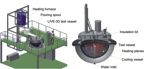
Figure 1 shows a schematic image of the LIVE facility.¹⁰ The main part of the LIVE test facility is a hemispherical lower head of a RPV of a typical pressurized water reactor in 1:5 scale.^9,11 The inner diameter of the test vessel is 1 m, and the wall thickness is ~25 mm. The material of the test vessel is stainless steel AISI316Ti, and its thermal properties are shown in Table I (Ref. 12). To investigate the influence of different external cooling conditions on the melt pool behavior, the test vessel is enclosed by a second vessel (cooling vessel) to enable ex-vessel cooling by water. The test vessel can be covered either by an insulation lid or by a cooling lid at the top. The decay heat in the melt is simulated by eight planes of electrical resistance heating wires, which can be controlled separately to realize homogeneous power generation in the melt pool. The distance between the heating planes and between the windings is 45 mm. The maximum possible homogeneous heat generation is 29 kW.

TABLE I Thermal Properties of Stainless Steel AISI316Ti*

Temperature (°C)	Thermal Conductivity (W/m/K)	Heat Capacity (J/kg/K)	Density (kg/m^3)
20	15	500	8000

*Reference 12.

Fig. 1. Scheme of the LIVE-3D facility and test vessel.¹⁰

To investigate the transient as well as the steady-state behavior of the simulated core melt, an extensive instrumentation of the test vessel was realized. The main instrumentation is the temperature measurement by thermocouples installed on the inner and outer vessel wall and inside the simulant melt. The temperature measurement can be divided into four categories:

1. wall temperature: 17 pairs of thermocouples at the inner surface (IT) and outer surface (OT) at the same position of the vessel wall

2. melt temperature: 74 thermocouples distributed in the bulk melt pool (MT and HT)

3. crust temperature or wall boundary temperature: six arrays of thermocouples, named CT trees

4. cooling water temperature and flow rate: two thermocouples for inlet and outlet water temperature (ZT and AT) together with mass flow meter (DF).

II.B. Test Condition of LIVE-J2

II.B.1. Simulant Materials

Two different simulant materials were used in the LIVE-J2 test. Ceramic beads and nitrate salt simulate the higher-melting-temperature oxidic components and the lower-melting-temperature metallic components, respectively. The ceramic spheric beads of RIMAX produced by ZIRPRO consisted of 58% ZrO₂ and 37% SiO₂, having the size of 2.5 to 2.8 mm. The nitrate salt was prepared at KIT, and a binary eutectic mixture of sodium nitrate and potassium nitrate was chosen as in other LIVE experiments. In the LIVE-J2 experiment, the eutectic composition of 50 mol % NaNO₃-50 mol % KNO₃ was selected, which has the eutectic temperature of 220°C to 222°C (Ref. 13). The thermal properties of ceramic beads and nitrate salt are described in Tables II and III, respectively.

TABLE II Thermal Properties of RIMAX*

Temperature (°C)	Thermal Conductivity (W/m/K)	Heat Capacity (J/kg/K)	Density (kg/m^3)
25	8.8	740	4100
250	7.7	1010	4013
500	7.2	1280	4018

*Reference 8.

TABLE III Thermal Properties of Nitrate Salt*

		Solid			Liquid	Reference
Mole weight (g/mol)		93.5
Thermal conductivity (W/m/K)		~0.42			~0.46	KIT estimation
Heat capacity (J/kg/K)		~1300			1492	Ref. 14
Density (kg/m^3)		−6.418·10^−Citation4·T + 2.193			−6.891·10^−Citation4·T + 2.112	Ref. 14
Transition temperature (°C)		113 to 115				Ref. 15
Thermal expansion rate (1/K)					1.5·10^−Citation4	Ref. 16
Transition/fusion enthalpy (J/g)		Δhtransition = 33.8, Δhfusion = 100.7				Ref. 15
Viscosity (Pa·s)				4.725·10^−3 (247°C) 3.893·10^−3 (317°C) 2.348·10^−3 (347°C)		Ref. 13
Temperature (°C)

*Nitrate salt = 50 mol %NaNO₃-50 mol %KNO₃; Ref. 8.

II.B.2. Test Performance

In the LIVE-J1 test that was conducted prior to the LIVE-J2 test, the uniformly mixed simulant debris of 245.4-kg ceramic beads and 79.6-kg nitrate salt fragments were preloaded in the test vessel.⁸ The total heating power of 10 kW was planned through the experiment, and no external and top cooling were applied in LIVE-J1. Due to the difference in the melting temperature, only the nitrate salt in the simulant debris bed melted and filled in the pores of the ceramic debris bed. The posttest endoscope analysis of LIVE-J1 inside the debris bed showed that almost all the nitrate melted down and no loose mixtures of ceramic or nitrate remained.

The LIVE-J2 test was performed on January 19 and 20, 2021, and the end state of the LIVE-J1 test was used as the initial condition of LIVE-J2, as shown in Fig. 2. Although the debris surface was almost flat at the elevation of about 280 mm from the inner bottom of the vessel, the height of the ceramic debris bed was slightly higher at the center and lower at the periphery. Thus, the nitrate salt existed above the ceramic debris bed at the periphery, as can be seen in Fig. 3. The LIVE-J2 test consisted of four heating phases, and the boundary conditions of each phase, as well as those of LIVE-J1, are given in Fig. 4.

Fig. 2. Initial debris contour with location of heating planes and thermocouples. Four MTs at one position indicate four thermocouples at the same radius and height, but distributed in 90-deg azimuth intervals.

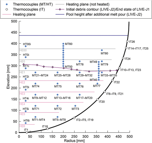
Fig. 3. Initial state of debris bed in LIVE-J2 (end state of LIVE-J1).

Fig. 4. Test matrix of the LIVE-J test series.

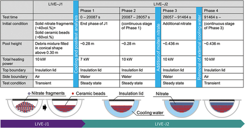
Throughout the test, the insulation lid was installed on the test vessel. The space between the debris surface and the insulation lid was filled with nitrogen gas with a flow rate of approximately 1 m³/h. Continuous cooling water with a flow rate of about 0.20 L/s was applied in the cooling vessel during the steady-state phases to remove the heat from the side wall. The average inlet and outlet temperatures during the steady-state phases were 9°C and 17°C, respectively.

In phases 1 and 2, the heat transfer behavior of the mixture pool under steady-state condition was investigated. The total planned heating power was 7 kW and 10 kW in phases 1 and 2, respectively. Since the heating plane HE1 was uncovered, five lower planes (HE2 to HE6) were used for decay heat simulation. After the end of phase 2, an additional 219 kg of nitrate was poured into the test vessel, and the melt height increased to about 436 mm. The heat transfer behavior of the two-layer molten pool was investigated in phase 3. Molten nitrate filled the pores of the ceramic beads and the heating was applied in the lower region, while a pure nitrate salt layer lay without heating in the upper region. After the steady state was reached, the external cooling water was removed and the transient behavior was observed in phase 4. At the time when the highest melting temperature reached 400°C, the power of all the heating planes was shut down.

II.C. Experimental Results

II.C.1. Steady State (Phase 1 and Phase 2)

The melting temperature evolution and the total heating power during the whole test are shown in Fig. 5. The actual heating power of each heating element is given in Table IV. The melting temperature contours at each time point are illustrated in Fig. 6. Although some photos and videos were recorded during the test, the information on the melt height evolution could not be obtained. Therefore, the surface contour measured after the LIVE-J1 test was used as the upper surface data for the melt distribution plots for phases 1 and 2. This surface is illustrated as a dashed line in phases 3 and 4. Figures 7 and 8 show the vertical temperature distributions in steady states at various vertical positions. The horizontal temperature profile is also shown in Fig. 9. The plotted values are the average of the different thermocouples located in different azimuths at the same radius and elevation.

TABLE IV Heating Power of Each Heating Plane in Each Phase

Heating Plane	Elevation (mm)	Heating Power in Phase 1 (W)	Heating Power in Phases 2, 3, and 4 (W)	Heater Diameter (mm)
HE00	381.4	0	0	4
HE0	332.4	0	0	4
HE1	282.4	0	0	4
HE2	234.4	2 973	4 224	4
HE3	186.4	1 558	2 256	4
HE4	136.4	1 206	1 716	4
HE5	89.4	1 092	1 564	3
HE6	36.4	202	294	2
Total power		7 032	10 054

Fig. 5. Melting temperature evolution and power input.

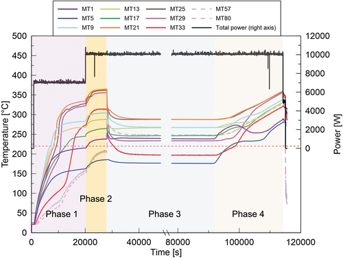
Fig. 6. Melting temperature distribution.

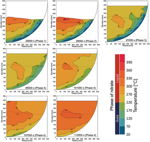
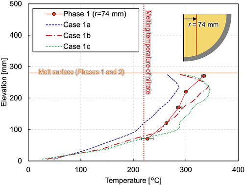
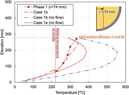
Fig. 7. Vertical melting temperature profile at radius of 74 mm in steady state.

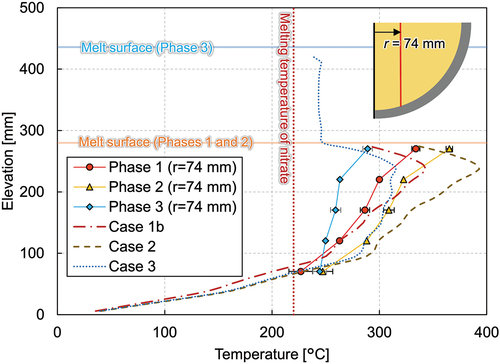
Fig. 8. Vertical melting temperature profile at radii of 360 mm and 374 mm in steady state.

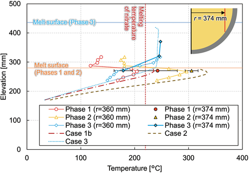
Fig. 9. Horizontal melting temperature profile at elevation of 170 mm.

At the steady state of phase 1, the temperatures at the elevation of 270 mm reached 327°C on average, except for the most peripheral thermocouple of MT33, which indicated 273°C. The temperature difference among MT21, MT25, and MT29 was approximately 10°C, which implies that the molten nitrate was well mixed in the central part of the molten pool. The melting temperature at the peripheral region at this elevation had a large discrepancy between 190°C and 273°C, depending on the azimuth (MT33, MT34, and MT35). A possible reason is the difference in the distribution of the ceramic beads. At the end of LIVE-J1, the ceramic beads submerged and a pure nitrate layer existed above the debris bed at the peripheral region (Fig. 3). At the azimuth angle of 90 deg, where the lower melting temperature was observed (MT34), more ceramic beads could be observed up to the most outer spiral of the heating wire compared to other azimuth angles. Another reason could be the solid mixture of ceramic and nitrate at the boundary due to the external cooling. Depending on the measured point in the liquid or in the solid boundary, the temperature difference can deviate to a large extent. As can be seen in Fig. 5, the melting temperature stratification was observed, and the middle thermocouple group (MT9, MT13, and MT17) at the elevation of 170 mm had lower temperatures than the temperatures at 270 mm. The horizontal temperature gradient was also observed at this elevation. The lowest thermocouples (MT1 and MT5) at the elevation of 70 mm indicate the solidification of nitrate, which shows the crust growth at this position. Local liquefaction, however, occurs near the heaters when the spiral heater element is in the solidified region.

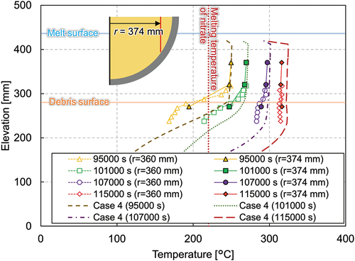
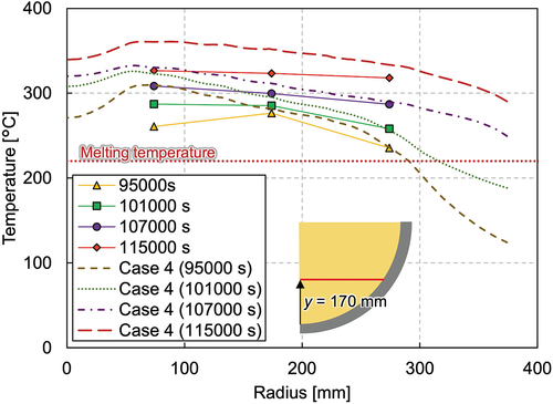
Figure 7 reveals the vertical temperature profile at the radius of 74 mm. The temperature gradient can be seen in the figure, and the temperatures ranged from 226°C near the vessel bottom to 335°C near the melt surface. In Fig. 8, the temperatures measured by the thermocouple tree at the radius of 360 mm located at azimuth angle of 320 deg and the average temperature at the radius of 374 mm are illustrated. The temperature at this location in phase 1 ranges around the melting temperature of nitrate, and the temperature differs significantly depending on the azimuth angles, as mentioned previously. An intensive analysis of the temperature measurements reveals the tendency for the temperatures along the azimuth at 0, 90, 180, and 270 deg to be similar to each other in the molten region, while the deviation is larger in the solidified area. Figure 9 shows the horizontal temperature gradient at the elevation of 170 mm, which implies convection is not fully developed in the mixture pool.

The crust thickness was estimated by the thermocouple trees installed at the inner vessel. As shown in Fig. 10, the crust formed along the vessel had a thickness of 70 to 80 mm in phase 1. The thickness at the bottom near the lowest heater wires is estimated to be quite thin compared to the region above. As previously mentioned, this is due to the localized effect that the region near the heater element is overheated.

Fig. 10. Crust thickness profile along inner vessel wall.

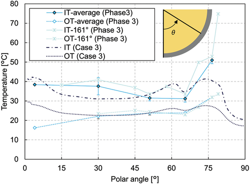
Figure 11 shows the vessel wall temperatures in phase 1. The bottommost thermocouples for the inner and outer wall measurements exist at the polar angle of 4 deg and at the azimuth of 292.5 deg. The vessel wall temperatures at the polar angles of 30, 51, 65.5, and 76.5 deg were measured by the thermocouples installed along four different azimuth angles at 22.5, 112.5, 202.5, and 292.5 deg. The average of these measurements is plotted in the figure, denoted as IT-average and OT-average for the inner and outer wall temperatures, respectively Additionally, nine thermocouples were attached along the azimuth in the range of 161 to 171 deg. These measurements are plotted separately in the figure, denoted as IT-161° and OT-161°. The melt surface lies at around 60 deg, which is slightly lower than the thermocouples installed at 65.5 deg (from IT10 to IT13). The inner wall average temperatures in phase 1 from the bottom to 51 deg were almost constant, which implies that the nitrate was uniformly cooled along the vessel wall and that conductive heat transfer was dominant near the vessel wall.

Fig. 11. Inner wall and outer wall temperature profiles along the vessel wall (phase 1).

In phase 2, increasing the heating power led to an increase of the overall melting temperature in the melt pool. Figures 7, 8, and 9 show that the melting temperature distribution in phase 2 had a similar trend to phase 1. The temperature at MT1 indicates that the nitrate remelted and the crust thickness reduced at this position. The temperature measurement at the peripheral region shows that the molten region developed in the horizontal direction as well (Fig. 9). The crust thickness reduced to ~40 mm at the region near the melt surface, whereas it was similar at the lower region compared to phase 1. The inner wall temperature, illustrated in Fig. 12, shows that the temperature at the polar angle of 51 deg was higher than those in the lower regions. Especially at the polar angle of 51 deg, the inner wall temperature reached 60°C. These facts indicate that heat transfer to the horizontal direction in the upper part of the molten pool became more significant in phase 2.

Fig. 12. Inner wall and outer wall temperature profiles along the vessel wall (phase 2).

II.C.2. Steady State with Additional Nitrate (Phase 3)

After the steady state was reached in phase 2, an additional 219 kg of nitrate was poured into the test vessel at 28 057 s, and phase 3 was initiated. The melt height increased up to 436 mm. Figure 7 shows the temperature gradient in the lower debris region where both the ceramic beads and nitrate exist. The nitrate was solidified at the peripheral region in the debris region, while it is molten and the uniform temperature distribution of about 250°C was indicated in the upper pure-nitrate region (Fig. 8). The horizontal temperature profile (Fig. 9) reveals that phase 3 had considerably lower temperatures and that the molten region was also smaller compared to phases 1 and 2.

Although the crust thickness at the polar angle of 37 deg was comparable in phase 3 and phase 1, the thermocouple trees inside the solidified region indicated a thicker crust thickness in the upper angles in phase 3. The crust thickness of the upper pure-nitrate region was considerably thinner than that of the lower debris region and was approximately around 9 mm (Fig. 10).

Figure 13 illustrates the vessel wall temperature in phase 3. The inner wall temperatures at the lower mixture region were rather decreasing with distance from the bottom. At the upper pure-nitrate region, in contrast, the inner wall temperature was significantly high. The test results showed that the heat generated in the lower mixture region was transferred upward to the upper pure-nitrate region. Since the melt was well mixed in the upper region, the heat transfer to the horizontal direction was also substantial, which heated up the vessel wall. Most of the heat removed by the external water could be from the upper region.

Fig. 13. Inner wall and outer wall temperature profiles along the vessel wall (phase 3).

II.C.3. Transient (Phase 4)

The external cooling water was removed at 91 464 s, and phase 4 was initiated. As seen in Fig. 5, the temperature increase up to 100 000 s at the lowermost thermocouples (MT1 and MT5) was rapid, while other thermocouples showed moderate temperature changes. At around 100 000 s, MT1 started to decrease and MT5 reached a plateau, whereas MT29 and MT33 instead indicated a rapid temperature increase. After 110 000 s, all thermocouples increased constantly in a similar trend. The thermocouples located in the upper pure-nitrate layer (MT57 and MT80) and those in the upper region of the mixture layer (MT21 and MT25) indicate a constant temperature increase through the transient phase. The thermocouples MT9, MT13, and MT17 installed in the middle region of the mixture layer also showed a constant increase with slight uneven changes at the beginning of the transient.

Figures 14 and 15 show vertical temperature profiles near the center and at the periphery, respectively. The lowermost thermocouples indicate temperature increases between 95 000 and 101 000 s and decreases between 101 000 and 107 000 s. On the contrary, the upper part of the thermocouples in the mixture region continuously increased. The temperature at the periphery region also changed largely between 101 000 and 107 000 s from ~210°C (below the melting temperature of nitrate) to ~280°C.

Fig. 14. Vertical melting temperature profile at radius of 74 mm in transient.

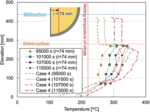
Fig. 15. Vertical melting temperature profile at radii of 360 mm and 374 mm in transient.

The horizontal temperature profile in Fig. 16 shows that the temperature at the periphery region increased significantly and that the temperature distribution flattened gradually. The melting temperature measurement data show that the molten area expanded downward at the beginning of the transient and then to the periphery afterward. The temperature evolution indicates that heat transfer was also enhanced to the horizontal direction in the upper part of the mixture region once the molten region was extended to the whole mixture region.

Fig. 16. Horizontal melting temperature profile at elevation of 170 mm.

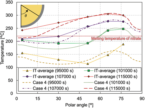
Figure 17 illustrates the inner vessel wall temperature profile at various time points, respectively. Up to 95 000 s, the inner wall temperature profile shows a “v” shape, having higher temperatures at the vessel bottom and the vessel side and a lower temperature at the vessel middle, which was the same trend as in phase 3. The vessel side temperature at 101 000 s increased above the melting temperature of nitrate, which indicates that the nitrate near the wall remelted and the crust disappeared in the upper pure-nitrate layer, as seen in Fig. 10. After 101 000 s, rapid changes along the vessel wall were observed; the crust thickness reduced quite quickly and disappeared by 107 000 s above the polar angle of 37 deg. At this time, the inner wall temperature reached values above the melting temperature of nitrate in most regions, except for the vessel bottom, indicating that most nitrate was molten. The melting temperature at the periphery was also significantly higher, as described earlier. The wall location at the pure-nitrate region had the highest temperature, and the highest inner vessel wall temperature was about 300°C at the time the heaters were shut down.

Fig. 17. Inner wall and outer wall temperature profiles along the vessel wall (phase 4).

III. NUMERICAL CALCULATION

III.A. Calculation Condition

A numerical simulation was conducted using the commercially available software Ansys Fluent (2020R2). The ceramic beads, nitrate, and test vessel were modeled in the calculation. Other structures, such as the external cooling vessel, the upper void region, and the insulation lid, were not modeled; they are considered the boundary conditions of external surfaces. Since the number of meshes increases dramatically if the mesh is generated with the round-shaped heater elements, as in the experiment, they are instead modeled in the quadrilateral shape. In order to reduce the number of meshes, the inside of the heater elements was not meshed and the heat flux was given at each surface.

A 30-deg sector model was used for the calculation, as shown in Fig. 18, which shows the lower debris height model for phases 1 and 2 and the higher debris height model for phases 3 and 4. The simulation result of the full-sector model was also compared with that of a sector model and is discussed later. A cross section of the mesh is also shown in the figure. The standard element size of 10 mm is used for the three-dimensional mesh generation. The element sizes were adjusted near the heater elements in the range of 3 and 6 mm according to the geometry of the heater element.

Fig. 18. Graphical representation of the boundary conditions and a cross section of the mesh.

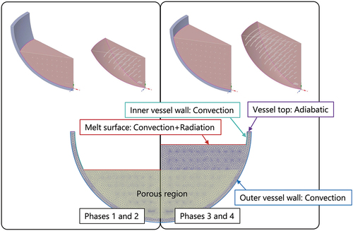
The boundary conditions used in the calculation are given in Table V and are also illustrated in Fig. 18. Convective heat transfer was assumed for the inner and outer vessel walls. As for the melt surface, both convective and radiation heat transfer conditions are given. The top edge of the vessel wall was assumed to be an adiabatic surface. The time-dependent reference temperatures in phase 4 are summarized in Table VI. The heating power of each heating plane was divided by the surface area of each heater geometry, and the total heat generation of 7 kW and 10 kW was given in the calculation in phase 1 and the later phases, respectively. The data of the thermal properties given in Tables I, II, and III were used in the calculation.

TABLE V Boundary Conditions and Calculation Matrix

		Outer Vessel Wall (Convection*1)^a		Inner Vessel Wall (Convection*2)^b		Melt Surface (Convection and Radiation*3)^c				Thermal Conductivity of Ceramic Beads
Simulation Case	Test Phase	Heat Transfer Coefficient h (W/m^Citation2/K)	Reference Temperature for Convection $T_{\mathrm{c}\mathrm{o}\mathrm{n}\mathrm{v}}$ (°C)	Heat Transfer Coefficient h (W/m^Citation2/K)	Reference Temperature for Convection $T_{\mathrm{c}\mathrm{o}\mathrm{n}\mathrm{v}}$ (°C)	Heat Transfer Coefficient h (W/m^Citation2/K)	Reference Temperature for Convection $T_{\mathrm{c}\mathrm{o}\mathrm{n}\mathrm{v}}$ (°C)	Emissivity $\epsilon$	Reference Temperature for Radiation $T_{\mathrm{r}\mathrm{a}\mathrm{d}}$ (°C)	$k$(W/m/K)	Geometry
Case 1a	Phase 1	500	11.8	10.0	166	10.0	166	1.00	154	7.70	Sector
Case 1b (base case)	Phase 1	500	11.8	10.0	166	10.0	166	1.00	154	3.09	Sector
Case 1c	Phase 1	500	11.8	10.0	166	10.0	166	1.00	154	1.54	Sector
Case 1d	Phase 1	500	11.8	10.0	166	10.0	166	1.00	154	3.09	Full
Case 1e	Phase 1	500	11.8	10.0	166	10.0	166	1.00	154	3.09	Full homogeneous heating
Case 2	Phase 2	500	13.6	10.0	219	10.0	219	1.00	201	3.09	Sector
Case 3	Phase 3	500	12.8	10.0	197	10.0	197	1.00	197	3.09	Sector
Case 4	Phase 4	10.0	$T_1\left(t\right)$	10.0	$T_2\left(t\right)$	10.0	$T_2\left(t\right)$	1.00	$T_3\left(t\right)$	3.09	Sector

^aThe average of the inlet (ZT) and the outlet (AT) cooling water temperature.

^bThe measured value of MT37 which is located above the melt surface.

^cThe measured value of DTi1 which is attached on the lower surface of the insulation lid.

TABLE VI Reference Temperatures for Convective and Radiation Boundaries in Phase 4

Time (s)	Outer Vessel Wall $T_1\left(t\right)$	Inner Vessel Wall and Melt Surface (Convection) $T_2\left(t\right)$	Melt Surface (Radiation) $T_3\left(t\right)$
92 000	24.7	197	196
95 000	50.8	202	201
98 000	68.1	211	208
101 000	79.1	223	219
104 000	87.0	237	232
107 000	94.5	249	245
110 000	101	262	258
113 000	106	275	272
115 000	108	64.5	62.5

The porous media model available in Ansys Fluent was used for the region where both the solid ceramic beads and solid/liquid nitrate exist. Porous media were modeled by the addition of a momentum source term to the standard fluid flow equations.¹⁷ The source term was composed of two parts. The first is a viscous term (Darcy), the first term on the right side of Eq. (1)(1) $S_i=-\left(\sum _{j=1}^3{D}_{ij}\mu v_j+\sum _{j=1}^3{C}_{ij}\frac{1}{2}\rho \left|v\right|v_j\right),$(1) :

(1) $S_i=-\left(\sum _{j=1}^3{D}_{ij}\mu v_j+\sum _{j=1}^3{C}_{ij}\frac{1}{2}\rho \left|v\right|v_j\right),$(1)

where

$S_i$	=	= source term for the i’th momentum equation
$\mu$	=	= viscosity
$\left|v\right|$	=	= magnitude of the velocity
D, C	=	= prescribed matrices.

The second part is an inertial loss term [the second term on the right side of Eq. (2)(2) $S_i=-\left(C_1\mu v_i+C_2\frac{1}{2}\rho \left|v\right|v_i\right),$(2) ]. This momentum sink contributes to the pressure gradient in the porous cell, creating a pressure drop that is proportional to the fluid velocity (or velocity squared) in the cell. In case of simple homogeneous media, Eq. (1)(1) $S_i=-\left(\sum _{j=1}^3{D}_{ij}\mu v_j+\sum _{j=1}^3{C}_{ij}\frac{1}{2}\rho \left|v\right|v_j\right),$(1) is simplified to

(2) $S_i=-\left(C_1\mu v_i+C_2\frac{1}{2}\rho \left|v\right|v_i\right),$(2)

where $C_1$ is the reciprocal of the permeability $\alpha$, and $C_2$ is the inertial resistance factor. The constants $C_1$ and $C_2$ are derived by using the Ergun equation,¹⁸ a semi-empirical correlation applicable over a wide range of Reynolds numbers:

(3) $\frac{\mathrm{\Delta }p}{L}=\frac{150\mu }{D_p^2}\frac{{\left(1-\varphi \right)}^2}{{\varphi }^3}{v}_{\mathrm{\infty }}+\frac{1.75\rho }{D_p}\frac{\left(1-\varphi \right)}{{\varphi }^3}{v}_{\mathrm{\infty }}^2,$(3)

where $L$ and $D_p$ are the bed depth and the mean particle diameter, respectively. The porosity (or void fraction) $\varphi$ is defined as the volume of voids divided by the volume of the packed bed region. A simplified version of the momentum equation, relating the pressure drop to the source term, can be expressed as

(4) $\mathrm{\nabla }p=S_i$(4)

or

(5) $\mathrm{\Delta }p=-S_i\mathrm{\Delta }n.$(5)

Hence, comparing Eqs. (2)(2) $S_i=-\left(C_1\mu v_i+C_2\frac{1}{2}\rho \left|v\right|v_i\right),$(2) and (3(3) $\frac{\mathrm{\Delta }p}{L}=\frac{150\mu }{D_p^2}\frac{{\left(1-\varphi \right)}^2}{{\varphi }^3}{v}_{\mathrm{\infty }}+\frac{1.75\rho }{D_p}\frac{\left(1-\varphi \right)}{{\varphi }^3}{v}_{\mathrm{\infty }}^2,$(3) ), the constants can be given as follows:

(6) $C_1=\frac{150}{D_p^2}\frac{{\left(1-\varphi \right)}^2}{{\varphi }^3}$(6)

and

(7) $C_2=2\times \frac{1.75}{D_p}\frac{\left(1-\varphi \right)}{{\varphi }^3}.$(7)

Since the diameter of the ceramic beads ranges between 2.5 and 2.8 mm, the average value of 2.65 mm was used for the mean particle diameter. The porosity of the ceramic beads was 0.3334 during the pretest analysis. Therefore, the constants $C_1$ and $C_2$ used in this study can be calculated from Eqs. (6)(6) $C_1=\frac{150}{D_p^2}\frac{{\left(1-\varphi \right)}^2}{{\varphi }^3}$(6) and (7(7) $C_2=2\times \frac{1.75}{D_p}\frac{\left(1-\varphi \right)}{{\varphi }^3}.$(7) ); they are $2.561\times {10}^8$ and $2.376\times {10}^4$, respectively.

The solidification and crust formation were calculated by the solidification/melting model available in Ansys Fluent, known as the enthalpy-porosity technique.^17,19 In this technique, the melt interface is not tracked explicitly. Instead, a quantity called the liquid fraction, which indicates the fraction of the cell volume that is in liquid form, is associated with each cell in the domain. The enthalpy of the material is computed as the sum of the sensible enthalpy $q$ and the latent heat $\mathrm{\Delta }H$:

(8) $H=q+\mathrm{\Delta }H.$(8)

The liquid fraction $\beta$ can be defined as

(9) $\begin{array}{rl}& \beta =0\mathrm{i}\mathrm{f}T<T_{\mathrm{s}\mathrm{o}\mathrm{l}\mathrm{i}\mathrm{d}\mathrm{u}\mathrm{s}}\\ & \beta =1if{T}_{\mathrm{l}\mathrm{i}\mathrm{q}\mathrm{u}\mathrm{i}\mathrm{d}\mathrm{u}\mathrm{s}}<T\\ & \beta =\frac{T-T_{\mathrm{s}\mathrm{o}\mathrm{l}\mathrm{i}\mathrm{d}\mathrm{u}\mathrm{s}}}{T_{\mathrm{l}\mathrm{i}\mathrm{q}\mathrm{u}\mathrm{i}\mathrm{d}\mathrm{u}\mathrm{s}}-T_{\mathrm{s}\mathrm{o}\mathrm{l}\mathrm{i}\mathrm{d}\mathrm{u}\mathrm{s}}}if{T}_{\mathrm{s}\mathrm{o}\mathrm{l}\mathrm{i}\mathrm{d}\mathrm{u}\mathrm{s}}<T<T_{\mathrm{l}\mathrm{i}\mathrm{q}\mathrm{u}\mathrm{i}\mathrm{d}\mathrm{u}\mathrm{s}}.\end{array}$(9)

The latent heat content can now be written in terms of the latent heat of the material $L$ as

(10) $\mathrm{\Delta }H=\beta L.$(10)

For solidification/melting problems, the energy equation is written as

(11) $\frac{\mathrm{\partial }}{\mathrm{\partial }t}\left(\rho H\right)+\mathrm{\nabla }\cdot \left(\rho vH\right)=\mathrm{\nabla }\cdot \left(k\mathrm{\nabla }T\right)+S.$(11)

The solution for temperature is essentially an iteration between the energy equation [Eq. (11(11) $\frac{\mathrm{\partial }}{\mathrm{\partial }t}\left(\rho H\right)+\mathrm{\nabla }\cdot \left(\rho vH\right)=\mathrm{\nabla }\cdot \left(k\mathrm{\nabla }T\right)+S.$(11) )] and the liquid fraction equation [Eq. (9)(9) $\begin{array}{rl}& \beta =0\mathrm{i}\mathrm{f}T<T_{\mathrm{s}\mathrm{o}\mathrm{l}\mathrm{i}\mathrm{d}\mathrm{u}\mathrm{s}}\\ & \beta =1if{T}_{\mathrm{l}\mathrm{i}\mathrm{q}\mathrm{u}\mathrm{i}\mathrm{d}\mathrm{u}\mathrm{s}}<T\\ & \beta =\frac{T-T_{\mathrm{s}\mathrm{o}\mathrm{l}\mathrm{i}\mathrm{d}\mathrm{u}\mathrm{s}}}{T_{\mathrm{l}\mathrm{i}\mathrm{q}\mathrm{u}\mathrm{i}\mathrm{d}\mathrm{u}\mathrm{s}}-T_{\mathrm{s}\mathrm{o}\mathrm{l}\mathrm{i}\mathrm{d}\mathrm{u}\mathrm{s}}}if{T}_{\mathrm{s}\mathrm{o}\mathrm{l}\mathrm{i}\mathrm{d}\mathrm{u}\mathrm{s}}<T<T_{\mathrm{l}\mathrm{i}\mathrm{q}\mathrm{u}\mathrm{i}\mathrm{d}\mathrm{u}\mathrm{s}}.\end{array}$(9) ].

III.B. Calculation Results

III.B.1. Phase 1

The calculation matrix as well as the boundary conditions are shown in Table VI. As for phase 1, five cases were compared to see the effects of the thermal properties and calculation geometries (see Appendix). Three calculations were conducted to compare the effect of the thermal conductivity of the ceramic beads. Since more than 66% of the domain was filled with ceramic beads, its thermal conductivity had a large influence on the heat transfer of the solid-liquid mixture pool. In case 1a, the thermal conductivity of the ceramic beads originally provided by the manufacturer (Table II) was used. The vertical temperature profile shown in Fig. 19 shows that the temperature is underestimated, which indicates that the generated heat is well transferred in the melt region and that the overall temperature was estimated lower than the measured values.

Fig. 19. Comparison of vertical melt temperature profiles at radius of 74 mm among the different thermal conductivities of the ceramic beads.

A mixing rule based on the volume fraction was used to estimate the thermal conductivity of the porous bed,

(12) $k_{eff}=\varphi k_{\mathrm{f}}+\left(1-\varphi \right)k_{\mathrm{s}},$(12)

where

$\varphi$	=	= porosity
keff	=	= effective thermal conductivities
$k_{\mathrm{f}}$	=	= fluid thermal conductivities
$k_{\mathrm{s}}$	=	= solid thermal conductivities.

By defining $\eta =k_{eff}/k_{\mathrm{f}}$ and $\kappa =k_{\mathrm{s}}/k_{\mathrm{f}}$, Eq. (12)(12) $k_{eff}=\varphi k_{\mathrm{f}}+\left(1-\varphi \right)k_{\mathrm{s}},$(12) can be written as follows:

(13) $\eta =\varphi +\left(1-\varphi \right)\kappa .$(13)

The measured values of k_eff, however, agree with the predictions made by Eq. (12)(12) $k_{eff}=\varphi k_{\mathrm{f}}+\left(1-\varphi \right)k_{\mathrm{s}},$(12) only if $k_{\mathrm{f}}\cong k_{\mathrm{s}}$ (Ref. 20). The larger the difference between the fluid and the solid thermal conductivities, the more the measured values of k_eff vary from the predictions made by Eq. (12)(12) $k_{eff}=\varphi k_{\mathrm{f}}+\left(1-\varphi \right)k_{\mathrm{s}},$(12) . The effective conductivity measurements in the past and the general difficulty encountered when attempting to develop a universal model are summarized in Ref. 21. The first and second Maxwell formulae,

(14) $\eta =\frac{2\varphi +\kappa \left(3-2\varphi \right)}{3-\varphi +\kappa \varphi }$(14)

and

(15) $\eta =\frac{2{\kappa }^2\left(1-\varphi \right)+\left(1+2\varphi \right)\kappa }{\left(2+\varphi \right)\kappa +1-\varphi },$(15)

are considered to be the most stringent lower and upper bounds for homogeneous, isotropic, two-phase mixtures.²² They are estimated for the conductivity of a composite medium having an unspecified phase distribution and could capture the relationship between the effective conductivity and the solid-fluid conductivity ratio when the conductivity ratio is small (1 $<\kappa <10$). In the case of LIVE-J2, the solid-fluid conductivity ratio (${\kappa }_{\mathrm{R}\mathrm{I}\mathrm{M}\mathrm{A}\mathrm{X}-\mathrm{n}\mathrm{i}\mathrm{t}\mathrm{r}\mathrm{a}\mathrm{t}\mathrm{e}}$) of the ceramic beads and nitrate is ~17. Compared with the measured data summarized in Ref. 21, it is still in the region where the effective fluid thermal conductivity ratio (${\eta }_{\mathrm{R}\mathrm{I}\mathrm{M}\mathrm{A}\mathrm{X}-\mathrm{n}\mathrm{i}\mathrm{t}\mathrm{r}\mathrm{a}\mathrm{t}\mathrm{e}}$) can be well predicted by Eq. (14)(14) $\eta =\frac{2\varphi +\kappa \left(3-2\varphi \right)}{3-\varphi +\kappa \varphi }$(14) . By applying the thermal conductivity of the ceramic beads of 7.7 and that of the nitrate of 0.46 to Eq. (14(14) $\eta =\frac{2\varphi +\kappa \left(3-2\varphi \right)}{3-\varphi +\kappa \varphi }$(14) ), the effective conductivity ($k_{eff(\mathrm{R}\mathrm{I}\mathrm{M}\mathrm{A}\mathrm{X}-\mathrm{n}\mathrm{i}\mathrm{t}\mathrm{r}\mathrm{a}\mathrm{t}\mathrm{e})}$) of 2.22 is obtained. Since Ansys Fluent calculates the effective thermal conductivity as the volume average of each material, as Eq. (12(12) $k_{eff}=\varphi k_{\mathrm{f}}+\left(1-\varphi \right)k_{\mathrm{s}},$(12) ), a $k_{\mathrm{R}\mathrm{I}\mathrm{M}\mathrm{A}\mathrm{X}}$ of 3.09 should give the effective conductivity of 2.22. For this reason, the thermal conductivity of the ceramic beads of 3.09 W/m/K is given in case 1b. As a comparison, that of 1.54 W/m/K was used in case 1c.

In case 1b, the temperature agrees quite well from the bottom to the middle at around the elevation of 170 mm, as illustrated in Fig. 7. Although the highest temperature is similar between the experiment and the simulation, its location has a difference of about 35 mm. The reason could arise from the different debris heights between the experiment and the calculation. A flat melt surface at the elevation of 275 mm is assumed in the calculation for simplicity, while the debris bed is higher as it reaches the center in the experimental geometry. At the radius of 74 mm, the debris height is about 305 mm. As the simulation results show, the highest temperature exists approximately 35 mm below the melt surface. Heat transfer to the atmosphere is effective near the debris surface. Considering the fact that the debris bed still exists above the uppermost thermocouple with a thickness of 35 mm in the experiment, it is reasonable that the uppermost thermocouple indicates the highest temperature in the experiment and that the elevation of highest temperature differs between the experiment and the simulation.

Additional plots of case 1b can be found in Figs. 8 through 11. The calculated temperature at the periphery has good agreement with the measured value (Fig. 8) and the horizontal temperature gradient observed in the experiment is also well simulated, as illustrated in Fig. 9, both of which are consistent with the result of the crust thickness estimation which agrees quite well with the measured data, except for the bottom (Fig. 10). The wall temperatures agree well where the polar angle is larger than 45 deg, while it is overestimated at the vessel bottom and underestimated in the middle region. During the LIVE-J1 test, the melting temperature at the very bottom of the vessel was below the melting temperature of nitrate, and the initial nitrate fragments are assumed to have remained unmolten. Heat transfer in this region should be worse compared to other regions where the nitrate had once been molten and filled the gap between the ceramic beads. The crust thickness agrees quite well at the polar angle of 37 deg, whereas the inner wall temperature is underestimated, which implies that heat transfer in the solidified region was underestimated. Thus, further consideration of effective thermal conductivity in the solidified region is necessary.

The thermal conductivity of 1.54 W/m/K was used for the ceramic beads in case 1c. From Fig. 19, it is obvious that the melting temperature was overestimated in all molten regions except for the location where the lowermost thermocouples exist, which implies that heat transfer is worse in the mixture region.

III.B.2. Phases 2, 3, and 4

Using case 1b as the base case, cases 2, 3, and 4 were calculated. The reference temperatures for the convective and radiation boundaries are given according to the cases by considering the measured values. Since case 4 is a transient case and the reference temperatures also changed against time, the time-dependent reference values are given. The calculated temperature and velocity contours are illustrated in Figs. 20 and 21, respectively.

Fig. 20. Calculated temperature contours.

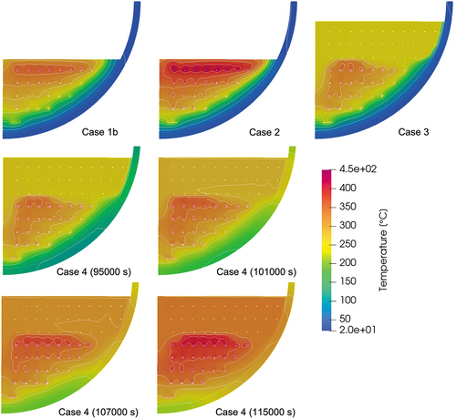
Fig. 21. Calculated velocity contour and vectors.

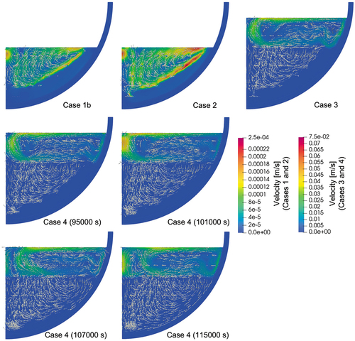
In case 2, which calculates phase 2 of the experiment, the temperature profiles (Figs. 7, 8, and 9) show that the calculated values are higher than the measured one in all regions. The crust thickness was generally well predicted, as shown in Fig. 10. Local liquefaction due to the existence of heater elements can clearly be seen at the three lower heater elements. The wall temperature (Fig. 12) distribution had a similar trend as in case 1b. As the total heating power was increased, the convective flow was enhanced and the inner wall temperature had a peak at around the polar angle of 58 deg near the melt surface.

The steady-state calculation with an additional pure-nitrate layer on top of the mixture layer is calculated in case 3. In the mixture layer, the calculated temperature is more than 50°C higher than the measured one at the radius of 74 mm (Fig. 7), while it agrees well with the experiment at the radii of 174 and 274 mm (Fig. 9). The pure-nitrate layer has a uniform melting temperature profile (compared in Fig. 8), which is also apparent from the calculated temperature contours in Fig. 20. As the velocity contour map in Fig. 21 shows, the velocity field of the upper layers is larger by two orders of magnitude compared to the lower layer, indicating the melt was well mixed in the pure-nitrate layer. In this study, laminar flow is assumed in all regions and no turbulence effect is considered. It is probable that turbulent flow occurs in the pure-nitrate layer and further investigation is necessary. The wall temperatures of the mixture region have a similar trend as in the previous cases and are generally well predicted (Fig. 13). A slightly thicker crust formation was predicted in the pure-nitrate layer, which affected the underestimation of the wall temperatures.

Case 4 calculates the transient phase of the experiment. The reference temperatures for the convective and radiation boundaries are time dependent and are given in Table VI. The predicted temperature evolutions at various probe locations are shown in Figs. 14, 15, and 16, which are compared with the measured data. As in case 3, the calculation results have a tendency to overestimate the temperatures in the central region of the mixture layer. The discrepancy between the experiment and the calculation is, however, smaller near the wall. On the other hand, the temperatures in the pure-nitrate layer are well predicted throughout the transient phase. The calculated inner wall temperatures are in a good agreement with the experimental temperature, especially after the crust disappeared and the inner wall temperature reached the melting temperature of nitrate. The highest wall temperature was located in the upper region and gradually moved downward as the whole melting temperature increased.

IV. SUMMARY AND CONCLUSIONS

In order to enhance understanding of the accident progression of 1F, it is certainly important to investigate the melting behavior of a number of control rod guide tubes (CRGTs) and CRD housing, which should have occurred before the formation of a molten pool in the lower plenum. At the time of vessel failure, however, it is estimated that most of metallic debris, including a forest of CRGTs and CRD housing, was already molten and that the oxide debris could also have been molten. Since vessel failure is originated from the heat up of the vessel wall, it is important to estimate the temperature profile of the vessel wall. Therefore, as a first step, the thermal behavior of the debris bed consisting of materials with different melting temperatures was experimentally investigated using the LIVE test facility. The previous LIVE-J1 experiment⁸ showed the melting behavior of solid nitrate and the development of a molten pool. In this paper, the results of the LIVE-J2 test are given. LIVE-J2 was conducted at KIT using two different simulant materials with different melting temperatures, and the experimental data on the thermal behavior of a solid-liquid mixture pool was enhanced. Additionally, a numerical calculation was performed using Ansys Fluent. Through the experimental and numerical analyses, the following conclusions have been obtained:

1. Although the conduction heat transfer is dominant along the cooled vessel wall, convective heat transfer also takes place to some extent in the molten region of the mixture pool and cannot be neglected. A quantitative analysis of how much convection is restricted by the existence of solid obstacles should be further conducted.

2. When a pure-nitrate layer exists on top of a solid-liquid mixture layer, horizontal heat transfer is better in the upper nitrate layer and the thermal load on the side wall will be larger. The highest wall temperature is located in the upper region and gradually moves downward as the whole melting temperature increases.

3. The influence of heater elements on melting temperature distribution is limited when a molten pool is formed. In the solid state where heat is transferred only by conduction, the heating method has a large effect on the heat-up behavior of the debris. This fact needs to be kept in mind when investigating the melting behavior of mixture debris.

4. In the LIVE facility, the radial flow is smaller in magnitude compared to the horizontal and vertical flows. A 30-deg sector model can capture the thermal behavior of the mixture pool.

5. The experimental and numerical investigation conducted in this study can enhance the understanding of heat transfer behavior in a solid-liquid mixture pool. The experimental results showed that the vessel wall temperature is higher at the upper part of the vessel wall, which supports the estimation that one or more larger openings could exist at the periphery of the lower head of 1F. For better prediction of the thermal behavior of a solid-liquid mixture pool, the experimental data also could be used for validation and improvement of numerical analysis tools, which could further deepen understanding of the vessel failure mechanism of the 1F.

Acknowledgments

The authors would like to express great appreciations to Mr. Akihiko Hashimoto and Mr. Kazuaki Sakae of NDD Corporation for their technical support on numerical analysis.

Disclosure Statement

No potential conflict of interest was reported by the authors.

APPENDIX

COMPARISON OF THE EFFECT OF DIFFERENT CALCULATION GEOMETRIES

The effect of different calculation geometries is compared, with case 1b calculated using a 30-deg sector model while case 1d uses a full-scale model. The vertical temperature profiles of both cases are illustrated in Fig. A.1. As each heater element has a spiral structure, the distance between the heater element and the probed location differs depending on the azimuth angles. Thus, the temperature profile varies among four locations. Especially at the azimuth of 270 deg, the heater elements locate at the radius of 74 mm of the probed location. Therefore, sharp temperature peaks can be seen in the plotting of case 1d (270 deg).

However, the temperatures where the thermocouple exists, that is between the heater elements, are similar among different azimuths. They also agree well with the temperature profile of a sector model (case 1b). A comparison of the solidification boundary is shown in Fig. A.2. Although a slight difference among the different azimuth angles exists, which is due to the spiral geometry of the heater element, the solidification profiles of a sector model and a full-scale model generally agree well. Comparing the temperature contours of the full-scale model, shown in Fig. A.3 (case 1d), and that of the scale-model, shown in Fig. 20 (case 1b), they agree qualitatively quite well.

The contour maps of the velocity magnitudes are also comparable. The upward flow can be seen in the central part of the molten region, and the melt flows horizontally near the melt surface to the side wall. Along the solidification boundary, large descending flow to the bottom was estimated. The flow in the radial direction was smaller than the vertical and horizontal flows and was considered to have little effect on the calculation results. Therefore, it can be concluded that a sector model is able to represent the facility and was used for calculations in later experimental phases.

Next, the influence of the heater elements on the temperature and flow distribution was studied. Case 1e is a full-scale model without heater elements. Heat is assumed to be generated homogeneously in the melt region. The other boundary conditions were kept the same. Comparing the vertical temperature profile of case 1b and that of case 1e in Fig. A.1, a maximum temperature difference of around 40°C can be found. The solidification boundary is formed smoothly as the local liquefaction by heater elements does not occur in the case of homogeneous heating (case 1e). In addition, the crust thickness was thicker in case 1e than in case 1b and case 1d. Figure A.3 illustrates the temperature and velocity contours of case 1d and case 1e. Though local heat up occurs near the heater elements in case 1d, similar lateral temperature expansion can be seen in both cases. The flow patterns are basically similar with upward flow in the middle and descending flow along the solidification boundary. In case 1d, local upward flow exists near the heater elements and the flow is more enhanced, which resulted in a larger magnitude of the flow velocity compared to case 1e.

Finally, two calculation cases solving only the energy equation are compared in Fig. A.4, specifically, case 1b (no flow), a sector model with heater elements, and case 1e (no flow), a full-scale model without heater elements (homogeneous heating). Since the momentum equation is not solved in these cases, only the conduction heat transfer was assumed in the simulant debris even above the melting temperature. Both cases overestimate the measured value and imply that convective heat transfer takes place to some extent in the solid-liquid mixture pool, which enhances both vertical and horizontal heat transfer. A large discrepancy, however, exists between two cases. In case 1b, the heat was released from the heater elements and was transferred to the simulant materials by conduction. Therefore, most heat was kept in the central region. On the other hand, in case 1e, heat generation was homogeneous in all simulant materials existing in the vessel and the generated heat was evenly distributed in the domain. This difference in heat transfer mechanism can be neglected when the domain is fully molten and the flow field is developed, while it has a large influence on the melting behavior.

Fig. A.1. Comparison of vertical melting temperature profiles at a radius of 74 mm among different calculation geometries.

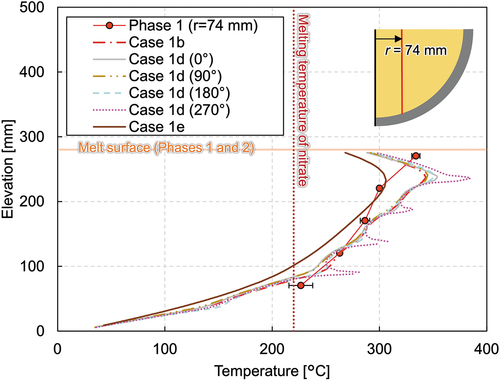
Fig. A.2. Comparison of crust thickness between different calculation geometries—case 1b: sector model, case 1d: full model, and case 1e: full model with homogeneous heating.

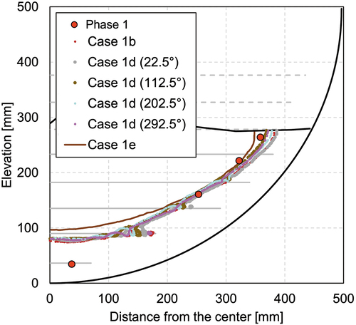
Fig. A.3. Comparison of temperature and velocity contours between the cases with and without heater elements.

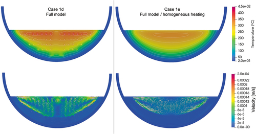
Fig. A.4. Vertical melting temperature profiles at a radius of 74 mm with an assumption of no-flow condition.

Acronyms

1F:	=	Fukushima Daiichi Nuclear Power Station
CRD:	=	control rod drive
CRGT:	=	control rod guide tube
KIT:	=	Karlsruhe Institute of Technology
LIVE:	=	Late In-Vessel Phase Experiments
PCV:	=	primary containment vessel
RPV:	=	reactor pressure vessel
TEPCO:	=	Tokyo Electric Power Company Holdings, Inc.

Nomenclature

$C$	=	= prescribed matrix
$C_1$	=	= reciprocal of permeability
$C_2$	=	= inertial resistance factor
$D$	=	= prescribed matrix
$D_p$	=	= mean particle diameter
$h$	=	= heat transfer coefficient
$k$	=	= thermal conductivity
$L$	=	= depth
$S$	=	= source term
$T$	=	= temperature
$t$	=	= time
$v$	=	= velocity

Greek

$\alpha$	=	= permeability
β	=	= liquid fraction
$\epsilon$	=	= emissivity
$\eta$	=	= ratio of effective and fluid thermal conductivities ($=k_{eff}/k_{\mathrm{f}}$)
$\kappa$	=	= ratio of solid and fluid thermal conductivities ($=k_{\mathrm{s}}/k_{\mathrm{f}}$)
$\mu$	=	= viscosity
$\varphi$	=	= porosity

Subscripts

conv	=	= convection
eff	=	= effective
f	=	= fluid
rad	=	= radiation
s	=	= solid

References

- M. PELLEGRINI et al., “Main Findings, Remaining Uncertainties and Lessons Learned from the OECD/NEA BSAF Project,” Nucl. Technol., 206, 9, 1449 (2020); https://doi.org/10.1080/00295450.2020.1724731.
- L. E. HERRANZ et al., “Overview and Outcomes of the OECD/NEA Benchmark Study of the Accident at the Fukushima Daiichi NPS (BSAF) Phase 2—Results of Severe Accident Analyses for Unit 1,” Nucl. Eng. Des., 369, 110849 (Oct. 2020); https://doi.org/10.1016/j.nucengdes.2020.110849.
- M. SONNENKALB et al., “Overview and Outcomes of the OECD/NEA Benchmark Study of the Accident at the Fukushima Daiichi NPS (BSAF), Phase 2—Results of Severe Accident Analyses for Unit 2,” Nucl. Eng. Des., 369, 110840 (2020); https://doi.org/10.1016/j.nucengdes.2020.110840.
- T. LIND et al., “Overview and Outcomes of the OECD/NEA Benchmark Study of the Accident at the Fukushima Daiichi NPS (BSAF), Phase 2—Results of Severe Accident Analyses for Unit 3,” Nucl. Eng. Des., 376, 111138, (2021); https://doi.org/10.1016/j.nucengdes.2021.111138.
- W. KLEIN-HESSLING et al., “Conclusions on Severe Accident Research Priorities,” Ann. Nucl. Energy, 74, 4, 4 (2014); https://doi.org/10.1016/j.anucene.2014.07.015.
- “Fukushima Daiichi Nuclear Power Station Unit 2 Primary Containment Vessel Internal Investigation Results,” Tokyo Electric Power Company Holdings, Inc., (2018); https://www.tepco.co.jp/en/nu/fukushima-np/handouts/2018/images/handouts_180201_01-e.pdf (current as of May 15, 2021).
- “Locating Fuel Debris inside the Unit 2 Reactor Using a Muon Measurement Technology at Fukushima Daiichi Nuclear Power Station,” Tokyo Electric Power Company Holdings, Inc. (2016); https://www.tepco.co.jp/en/nu/fukushima-np/handouts/2016/images/handouts_160728_01-e.pdf (current as of Jan. 30, 2020).
- H. MADOKORO et al., “LIVE-J1 Experiment on Debris Melting Behavior Toward Understanding Late In-Vessel Accident Progression of the Fukushima Daiichi Nuclear Power Station,” Proc. 19th Int. Topl. Mtg. on Nuclear Reactor Thermal Hydraulics (NURETH-19), Brussels, Belgium (2022).
- F. KRETZSCHMAR and B. FLUHRER, Behavior of the Melt Pool in the Lower Plenum of the Reactor Pressure Vessel—Review of Experimental Programs and Background of the LIVE Program, Vol. FZKA-7382, Forschungszentrum Karlsruhe (2008).
- X. GAUS-LIU et al., “Experimental Study on the Melt Pool Transient Behaviour in LWR Lower Head Under Changing Boundary Cooling Conditions: The Outcomes of LIVE-ALISA Experiment,” presented at the 12th Int. Topl. Mtg. on Nuclear Reactor Thermal-Hydraulics, Operation and Safety (NUTHOS-12), Qingdao, China (2018).
- X. GAUS-LIU et al., “In-Vessel Melt Pool Coolibility Test—Description and Results of LIVE Experiments,” Nucl. Eng. Des., 240, 11, 3898 (2010); https://doi.org/10.1016/j.nucengdes.2010.09.001.
- “AISI316Ti Data Sheet,” M. WOITE GMBH (2012);https://woite-edelstahl.com/aisi316tien.html (current as of Mar. 27, 2022).
- G. J. JANZ et al., Physical Properties Data Complications Relevant to Energy Storage II. Molten Salts: Data on Single and Multi-component Salt Systems, U.S. Government Printing Office, Washington, District of Columbia (1979); https://nvlpubs.nist.gov/nistpubs/Legacy/NSRDS/nbsnsrds61p2.pdf.
- T. BAUER, D. LAING, and R. TAMME, “Overview of PCMs for Concentrated Solar Power in the Temperature Range 200 to 350°C,” Adv. Sci. Technol., 74, 272 (2010); https://doi.org/10.4028/www.scientific.net/ast.74.272.
- D. J. ROGERS and G. J. JANZ, “Melting-Crystallization and Premelting Properties of NaNO3-KNO3. Enthalpies and Heat Capacities,” J. Chem. Eng. Data, 27, 424 (1982); https://doi.org/10.1021/je00030a017.
- G. D. SAO and H. V. TIWARY, “Thermal Expansion of Potassium Nitrate Films,” Jpn. J. Appl. Phys., 20, 3, L225 (1981); https://doi.org/10.1143/JJAP.20.L225.
- “ANSYS Fluent User’s Guide (2020R2),” ANSYS Inc. (2020).
- S. ERGUN, “Fluid Flow Through Packed Columns,” Chem. Eng. Prog., 48, 2, 89 (1952).
- V. R. VOLLER and C. PRAKASH, “A Fixed-Grid Numerical Modeling Methodology for Convection-Diffusion Mushy Region Phase-Change Problems,” Int. J. Heat Mass Transfer, 30, 8, 1709 (1987); https://doi.org/10.1016/0017-9310(87)90317-6.
- V. PRASAD et al., “Evaluation of Correlations for Stagnant Thermal Conductivity of Liquid-Saturated Porous Beds of Spheres,” Int. J. Heat Mass Transfer, 32, 9, 1793 (1989); https://doi.org/10.1016/0017-9310(89)90061-6.
- H. T. AICHLMAYR and F. A. KULACKI, “The Effective Thermal Conductivity of Saturated Porous Media,” presented at the 2005 ASME Summer Heat Transfer Conf. (HT2005), San Francisco, California (2005); https://doi.org/10.1016/S0065-2717(06)39004-1.
- G. R. HADLEY, “Thermal Conductivity of Packed Metal Powders,” Int. J. Heat Mass Transfer, 29, 6, 909 (1986); https://doi.org/10.1016/0017-9310(86)90186-9.