Air connectivity and regional employment: a spatial econometrics approach

ABSTRACT

While there is ample evidence for the existence of positive wider economic impacts of air transportation, the associated spatial distribution of these impacts has received less attention. This paper uses a spatial–econometric approach with instrumental variables on European NUTS-3-level panel data to study the spatial distribution of the impacts of air transport access on a subset of service-sector employment that is not directly affected by activity in the aviation industry. While the spatially resolved approach confirms previous findings that regions close to an airport experience service-sector employment increases due to improved air transport access, we also find evidence for the presence of an agglomeration shadow, that is, negative employment effects for regions further away from an airport. The average total impact of connectivity increases on service employment is found to be positive.

KEYWORDS:

• transportation
• aviation
• economic geography
• agglomeration

JEL:

• F63
• O18
• R12

INTRODUCTION

Airports serve as access points to a global network of air travel and air logistics. Consequently, they are perceived as an essential tool for regional development by helping regions overcome geographical disadvantages and connecting them with other centres of economic activity. Existing empirical work on the impacts of air transportation on regional development primarily builds on the seminal work by Brueckner (2003), who studies the region-by-region employment impacts of aviation as an enabler for face-to-face interactions and productivity. In their review of empirical studies on the wider economic impact of aviation, Lenaerts et al. (2021) find that most studies confirm the existence of positive economic impacts of air transport links, with recent evidence by Sheard (2019), Fageda and Olivieri (2019) and Campante and Yanagizawa-Drott (2018). Against this background, regional policymakers in Europe and elsewhere are investing in airport infrastructure and providing support to airlines for new or improved air services (Allroggen et al., 2013).

The associated spatial distribution of the benefits has received less attention (Cidell, 2015). This is an issue as airports’ impact on their hinterland can be assumed to be heterogeneous over space since airports are point infrastructure assets and users need access to this point infrastructure to benefit from its services. More specifically, while improving air transport can benefit nearby firms, it might also attract firms from regions further away from the airport, thereby negatively impacting economic activity in more distant regions. Therefore, both scholars and policymakers need to understand which regions benefit from increased air connections – or in other words: how far potential positive impacts of air services from an airport will reach and at which point they might become negative.

One of the first articles to address the spatial reach of airports’ economic impacts is Percoco (2010), who studies the impacts of air transport availability on Italy’s service-sector employment. Percoco (2010) addresses spatial modelling in response to concerns over selection bias resulting from assigning zero air traffic to regions with no airport. The latter is significant since a single airport can have multi-region or even multi-nation catchment areas (Lieshout, 2012), suggesting that a single airport often serves regions that are larger than small administrative units (here, Italian provinces). Percoco (2010) subsequently proposes calculating each region’s access to air transport through a spatial weight matrix based on inverse-distance squared, which models a hypothesized predetermined attenuation of economic benefits with airport access distance.

Scholars have also questioned whether the regional economic benefits of transport system improvements result from additional economic activity such as increased wages, population and employment, trade, and industry composition, or from spatial reallocation of economic activity between regions (Redding & Turner, 2015). Fageda and Gonzalez-Aregall (2017) address this question while estimating the regional economic impacts of different transportation modes (including aviation) in 47 Spanish provinces (NUTS-3 regions) between 1995 and 2008. For this purpose, they use a spatial Durbin model, which considers spatial dependencies in the dependent and independent variables based on weight matrices constructed using contiguity and three different distance-based cut-off levels (150, 300 and 450 km). They do not find a significant effect of air freight on employment for local and neighbouring airports. Similarly, Fageda and Olivieri (2019) quantify the impact of infrastructure for different transportation modes on per capita gross domestic product (GDP) growth in Spain between 1980 and 2008. Their spatial Durbin model considers weight matrices constructed using either contiguity, squared distance and the five nearest neighbours. By analysing the differential impact of transport infrastructure in each respective region and in neighbouring regions, the authors conclude that only roads have contributed to economic growth in Spain.

Campante and Yanagizawa-Drott (2018) estimate the impact of aviation on night lights at the grid-cell level¹ for a sample of 819 cities worldwide. Instead of using a spatial weights matrix, they include distance to the nearest airport as a regressor, which allows them to assess the rate at which the positive economic effects attenuate with distance. They also run their model for subsamples constructed from pixels within a rolling window of distance to the nearest airport up to 500 miles. They find significant positive effects close-by and smaller insignificant negative effects further away from the airport. The authors, therefore, conclude that improved air market access induces spatial inequality (i.e., regions closer to better-connected airports grow faster) rather than pure spatial reallocation.

While these existing studies on the economic impacts of aviation shed some light on the spatial nature of regional economic impacts of aviation, we are not aware of studies that systematically estimate the spatial reach of those benefits while also considering potential shadow effects on regions further away from an airport. This analysis aims to address this gap by developing spatial–econometric models combined with fine-scale employment data for European NUTS-3 regions. The European context is well-suited to study the spatial–economic impact of aviation because (1) distances between European regions are low while economic activity is spread out (geographically dispersed) but strongly interconnected (Combes & Overman, 2004); and (2) commercial airport density is relatively high (Poelman, 2013). In such a setting, ignoring spatial distributions can lead to estimation bias when quantifying aviation’s economic impact. This contrasts with the US context, where the co-location of airports and economic activity in metropolitan areas reduces the importance for spatially explicit analyses. In addition, our analysis controls for potential empirical biases resulting from parameter endogeneity by proposing a set of instrument variables derived from the aviation network through which air connectivity is generated.

We expect our findings to inform policymaking concerning regional airport development. This is because an uneven distribution of airports implies that transport improvements can create winner and loser regions, either relatively or absolutely. Our results can contribute to providing insight into the question whether regions without a local airport might suffer a competitive disadvantage. Additionally, our research can identify the spatial scope of airports’ economic impact, which can provide guidance on the allocation of state funds from the national to the local level.

The remainder of the paper is structured as follows. The next section provides insights into the mechanisms that drive the geographical dependencies between regions and the impact of transportation on economic systems. The third section introduces the spatial models to estimate the strength and spatial extent of economic geography effects for lagged air connectivity. The fourth section discusses the data. The fifth section discusses the results of the various spatial econometric approaches. The final section concludes.

TRANSPORTATION AND ECONOMIC GEOGRAPHY

Quantifying the economic impact of transportation requires an understanding of the economic mechanisms that result from transport services improving access to markets. Lenaerts et al. (2021) provide a theoretical overview of these mechanisms, leveraging the New Economic Geography (NEG) (Fujita et al., 1999; Krugman, 1991), the literature on inter-organizational collaboration and innovation (Boschma, 2005; Knoben & Oerlemans, 2006) and the general economic geography of transportation (Allroggen, 2013; Lakshmanan, 2011). Based on their review and extending the NEG framework, they identify six economic mechanisms, which ultimately shape the economic impact of transportation systems on affected regions. First, with decreasing transport costs resulting from better access to transportation, firms will leverage internal economies of scale by agglomerating production in nodes central to both their supply and demand networks (demand or backward linkages). Second, transportation makes agglomerations more attractive places of residence because consumers have an incentive to settle in cities or regions with favourable access to significant markets (cost or forward linkages). Third, as reductions in transportation costs can result in gains for some regions (agglomeration effect), this growth can be fuelled by reducing economic activity in other regions (agglomeration shadow). The reason behind this is that more accessible regions often outcompete less accessible regions. Fourth, congestion, pollution and the scarcity of nontraded consumption goods and services (driving up prices and wages) create a pull force for firms and consumers away from the congested agglomeration into less congested but less accessible or smaller urban centres (agglomeration spillover). The result is that hierarchal agglomeration characterized by multiple-centre geographies can be favoured with low transportation costs. Fifth, if transportation induces agglomeration of both firms and workers, which in turn drives agglomeration, the cost and demand linkages outlined above create a system of circular causation. Lastly, scale economies in transportation and multiplier effects of demand-side economics co-occur with the supply-driven impacts of transportation.

Over the last two decades, substantial empirical evidence highlighting the importance of (new) economic geography theories and its underlying mechanisms as outlined above has accumulated, specifically on (1) the relevance of market access for income and production, (2) the strength of agglomeration forces and (3) how agglomeration economies attenuate with distance (Combes & Gobillon, 2015; Head & Mayer, 2004; Redding & Rossi-Hansberg, 2017; Redding & Turner, 2015; Rosenthal & Strange, 2004). Furthermore, a subset of the empirical literature has focused on assessing the ‘spatial scope’ of economic geography effects. Examples include studies on the role of proximity in shaping agglomeration economies in different sectors (Rosenthal & Strange, 2003; Dekle & Eaton, 1999; Duranton & Overman, 2005), innovation (Jaffe et al., 1993), labour markets (Mion, 2004; Patacchini & Zenou, 2007; Hanson, 2005) and population (Redding & Sturm, 2008). Most studies find significant dependencies and agglomeration effects that are relatively localized. A notable study of transportation effects is Hodgson (2018) who provide evidence that regions located within 5 km to a railroad connection have higher survival probability and expected lifetime of US post offices, while railroad construction between 5 and 10 km of an existing post office decreases the survival probability and expected lifetime. Yet, more empirical evidence is needed that quantifies the spatial scope to distinguish agglomeration growth effects from mechanisms that affect economic activity negatively such as reorganization and competition between cities or regions (as hypothesized by theory).

Two elements are needed to apply the above economic geography theories to air transport and to estimate aviation’s spatial–economic impact. First, a method for mapping airports to their impacted regions is needed, which would enable the analysis of the spatial scope of airports’ economic impact and potential shadow effects. This is particularly important in Europe’s dense airport network, where airports can serve multiple regions and can have impacts beyond the region they are located in. Second, air market access needs to be calculated considering connecting flights generated through air networks. We capture market access generated by aviation in the form of ‘air connectivity’, which accounts for the quality of air transport services as a means to overcome distances and the quality of the destination market (Lenaerts et al., 2021). Air connectivity can be generated through direct (non-stop) flights and indirect (one- or multi-stop) connections that require passengers to transfer to a connecting flight at a hub airport to reach their final destination.

METHOD

We set out to develop a model to empirically test the hypothesized impacts of airport access. For each region, we explain a subset of service employment outcomes (our measure of economic activity) through (1) the air service supply of airports in the region (demand linkages); (2) the air service supply of neighbouring airports (demand linkages, agglomeration shadow and spillover); (3) economic activity, namely employment, in neighbouring regions (demand linkages, agglomeration shadow and spillover); and (4) other characteristics of the region. Besides the option to analyse potential regional spillovers in employment, we include (lagged) employment in neighbouring regions to disentangle air market impacts from the effects following access to centres of employment and to compare the spatial patterns of both effects. This is justified as both physical proximity to centres of service employment and air connectivity provide access to information and people (rather than goods).

Model specification

Spatial–econometric model

Although it is possible to include spatial lags in the dependent variable, independent variables, and error terms simultaneously, such models are difficult to estimate and interpret (Manski, 1993). We follow Elhorst (2010) and LeSage and Pace (2009) by dropping the spatial interaction effects among the error terms, resulting in the spatial Durbin model. Following Elhorst (2010) and LeSage and Pace (2009), the spatial Durbin model offers three advantages: (1) it produces unbiased coefficient estimates even if the true data-generation process differs;² (2) it reduces omitted variables bias (common in regional data samples); and (3) it produces unbiased standard errors even if the true data-generating process contains spatial dependence in the error term.

Due to the availability of space–time (panel) data, we use the time–space recursive version of the spatial Durbin model (LeSage & Pace, 2009), where, following Redfearn (2009), the temporal lag in employment is dropped due to multicollinearity (see Figure A4 in Appendix A in the supplemental data online). To control for aggregate missing variables that affect both local outcomes and local characteristics, we consider country-level fixed-effects (Combes & Gobillon, 2015). Given space–time data of adjacent spatial units, Elhorst (2014) reports that the fixed effects model is generally more appropriate than the random-effects model.

We propose a simplified model focusing on airport interaction only (equation 1, capturing (1) and (2)) and a full model incorporating airport (connectivity) and regional (employment) interaction (equation 2, capturing (1)–(3)).³ (1) $Empl=\alpha {\iota }_n+\beta \mathbf{V}Conn+{\mathbf{X}}_{\mathrm{c}}{\theta }_c+{\mathbf{X}}_{\mathrm{g}}{\theta }_g+{\mathbf{X}}_{\mathrm{t}}{\theta }_t+u$(1) (2) $\begin{array}{rl}Empl=& \alpha {\iota }_n+{\rho }_{\mathrm{near}}{\mathbf{W}}_{\mathrm{near}}LEmp{l}^S+{\rho }_{\mathrm{far}}{\mathbf{W}}_{\mathrm{far}}LEmp{l}^S\\ & +{\beta }_{\mathrm{near}}{\mathbf{V}}_{\mathrm{near}}Conn+{\beta }_{\mathrm{far}}{\mathbf{V}}_{\mathrm{far}}Conn\\ & +{\mathbf{X}}_{\mathrm{c}}{\theta }_c+{\mathbf{X}}_{\mathrm{g}}{\theta }_g+{\mathbf{X}}_{\mathrm{t}}{\theta }_t+u\end{array}$(2) The $n\times 1$ vector $Empl$ contains the dependent variable: a subset of service employment that is not directly affected by activity in the aviation industry (in absolute numbers). $n$ represents the number of observations at the regional level and is defined as $n=p\times t$ where p represents the number of NUTS-3 regions and t number of years t considered. ${\mathbf{X}}_{\mathbf{c}}$ represents the $n\times k$ matrix of all $k$ (exogenous) control variables, with associated parameters ${\theta }_c$ contained in a $k\times 1$ vector. ${\mathbf{X}}_{\mathbf{g}}$ represents the$n\times g$ matrix relating the $g\times 1$ vector of country-fixed effects ${\theta }_g$ to $Empl$. ${\mathbf{X}}_{\mathbf{t}}$ represents an$n\times t$ matrix relating the $t\times 1$ vector of time-fixed effects ${\theta }_t$ to employment in all time periods $t$. We include the vector of ones ${\iota }_n$ and associated parameter α since $Empl$ is not assumed to have a mean value of zero (LeSage & Pace, 2009). The $m\times 1$ vector Conn contains our impact variable connectivity and β is a scalar parameter. $m$ represents the number of observations at the airport level and is defined as $m=k\times t$ where k represents the number of airports. The $n\times m$ spatial weight matrix V links every region to its neighbouring airports. $LEmp{l}^S$ represents the one-year time lag in employment; $Emp{l}^S$ differs from $Empl$ by replacing missing values by the population-weighted share of employment at the NUTS-2 level.

In equation (2), the $n\times n$ matrices ${\mathbf{W}}_{\mathrm{near}}$ and ${\mathbf{W}}_{\mathrm{far}}$ link every region to its neighbouring regions, while the $n\times m$ matrices ${\mathbf{V}}_{\mathrm{near}}$ and ${\mathbf{V}}_{\mathrm{far}}$ link every region to its neighbouring airports (including its own). More specifically, the matrices ${\mathbf{W}}_{\mathrm{near}}$ and ${\mathbf{V}}_{\mathrm{near}}$ consider links to first-order neighbour regions and airports only, whereas ${\mathbf{W}}_{\mathrm{far}}$ and ${\mathbf{V}}_{\mathrm{far}}$ link to second-order neighbours. First-order neighbours are regions close to a specific region – that is, direct neighbours or regions within a short distance (see the third section for parameterizations). Second-order neighbours are close to the first-order neighbours (see the third section for parameterizations). We note that for second-order neighbour connectivity impacts, we consider the first-order connectivity value of each second-order neighbouring region instead of considering the connectivity values in each airport. This approach allows us to consistently assess the attenuation of benefits and potential adverse shadow effects, that is, both first- and second-order lagged connectivity represent the connectivity that is accessible to a region relative to other regions. The specification of the spatial weight matrices is discussed in the following subsection. The scalars ${\rho }_{\mathrm{near}}$, ${\rho }_{\mathrm{far}}$, ${\beta }_{\mathrm{near}}$ and ${\beta }_{\mathrm{far}}$ represent the respective parameters.

Spatial weights matrix specification

Our spatial weight matrices capture (1) employment in neighbouring regions, depending on proximity, and (2) the air service supply of airports within a region (depending on contiguity) or outside a region (depending on distance). These weight matrices can be defined based on (1) contiguity, (2) distance and (3) area (Figure 1). These approaches are combined with the simplified and full model (equations 1 and 2) to yield five model specifications (see Table 1 for a summary).

Figure 1. Allocation of NUTS-3 regions and airports (summed at the regional level) to first-order (grey) and second-order (black) neighbouring zones according to contiguity, distance (using point coordinates) and areal share.

Note: Dots represent the centre of the impact region (as an example, the DE732 region in Germany was taken). Triangles represent airports. Germany is only shown as an example, and we note that our full dataset contains all European NUTS-3 regions.

Sources: Border data from Eurostat GISCO (2019); and regional centres from Oak Ridge National Laboratory (ORNL) (2019).

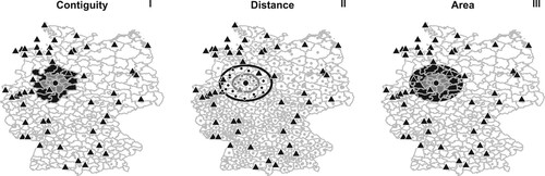
Table 1. Overview of models considered.

Model	Model type	Spatial weight matrix
A	First-order airport interaction only (equation 1)	Binary matrix $\mathbf{V}$ with ${\mathrm{V}}_{ik}=1$ if airport k lies within region i
B	First-order airport interaction only (equation 1)	Binary matrix $\mathbf{V}$ with ${\mathrm{V}}_{ik}=1$ if ${\mathrm{d}}_{\mathrm{ik}}$ is minimal
C	First- and second-order regional and airport interaction (equation 2 and specification I from Figure 1)	Binary matrix ${\mathbf{W}}_{\mathrm{near}}$ with ${\mathrm{W}}_{\mathrm{near},ij}=1$ if regions i and j share boundaries (queen-type) (green regions) Binary matrix ${\mathbf{W}}_{\mathrm{far}}$ with ${\mathrm{W}}_{\mathrm{far},ij}=1$ if region j shares boundaries with the green regions (except i) (queen-type) (red regions) Binary matrix ${\mathbf{V}}_{\mathrm{near}}$ with ${\mathrm{V}}_{\mathrm{near},ik}=1$ if airport k lies in a green region (including i) Binary matrix ${\mathbf{V}}_{\mathrm{far}}={\mathbf{W}}_{\mathrm{far}}\cdot {\mathbf{V}}_{\mathrm{near}}$
D	First- and second-order regional and airport interaction (equation 2 and specification II from Figure 1)	Binary matrix ${\mathbf{W}}_{\mathrm{near}}$ with ${\mathrm{W}}_{\mathrm{near},ij}=1$ if ${\mathrm{d}}_{\mathrm{ij}}<$ cut-off Binary matrix ${\mathbf{W}}_{\mathrm{far}}$ with ${\mathrm{W}}_{\mathrm{far},ij}=1$ if ${\mathrm{d}}_{\mathrm{ij}}>$ cut-off and ${\mathrm{d}}_{\mathrm{ij}}<$ outer limit Binary matrix ${\mathbf{V}}_{\mathrm{near}}$ with ${\mathrm{V}}_{\mathrm{near},ik}=1$ if ${\mathrm{d}}_{\mathrm{ik}}<$ cut-off Binary matrix ${\mathbf{V}}_{\mathrm{far}}={\mathbf{W}}_{\mathrm{far}}\cdot {\mathbf{V}}_{\mathrm{near}}$
E	First- and second-order regional and airport interaction (equation 2 and specification III from Figure 1)	Non-binary matrix ${\mathbf{W}}_{\mathrm{near}}$ with ${\mathrm{W}}_{\mathrm{near},ij}$ the share of region j within a circle around region i (radius = cut-off; green zone) Non-binary matrix ${\mathbf{W}}_{\mathrm{far}}$ with ${\mathrm{W}}_{\mathrm{far},ij}$ the share of region j within a concentric ring around region i (bandwidth = outer limit – cut-off; red zone) Binary matrix ${\mathbf{V}}_{\mathrm{near}}$ with ${\mathrm{V}}_{\mathrm{near},ik}=1$ if ${\mathrm{d}}_{\mathrm{ik}}<$ cut-off Binary matrix ${\mathbf{V}}_{\mathrm{far}}={\mathbf{W}}_{\mathrm{far}}\cdot {\mathbf{V}}_{\mathrm{near}}$

In model A, we aim to analyse the employment effects of airports in their ‘home region’ only. Therefore, airport allocation is based on all airports within a single NUTS-3 region’s boundaries (contiguity). Percoco (2010) shows that this approach is potentially subject to selection bias and might misrepresent airport usage patterns (multi-region catchment areas). In model B, airport allocation is based on the single nearest airport (distance) to gain insights into such bias.

In the remaining three models, we set out to assess the spatial structure of both regional dependencies in economic activity and the economic impacts of airports. More specifically, we disentangle the likely positive effects of first-order neighbours and their airports from the impacts of second-order neighbours and their airports, as outlined in equation (2). In model C, we define first- and second-order neighbours according to (queen-type) contiguity. For air connectivity, airports are allocated to regions and considered accordingly. This specification is potentially subject to bias resulting from the arbitrary delineation of region borders.

Thus, in model D, we define first- and second-order neighbours using the distance between the centres of each region under consideration and all other regions using cut-off values that are varied as part of the study. This cut-off serves as the inner limit (maximum distance) to the first-order neighbours; equivalently, an outer limit needs to be defined for the second-order neighbours (e.g., to cut off the potential scope of agglomeration shadow effects). The spatial weight matrices of air connectivity are defined accordingly. For regions with dispersed economic activity, this method can induce bias, as it might misclassify significant economic activity not located at the centre of a region.

In model E, each region’s area share that lies within concentric circles and concentric rings centred at each region under consideration is calculated for a range of radii (Rosenthal & Strange, 2003). First-order neighbours for employment are defined as the share of all regions falling within aforementioned concentric circles and second-order neighbours as they fall within the aforesaid concentric rings. Next, first-order neighbours for connectivity are defined as all airports within a certain cut-off distance from the region under consideration. The second-order neighbours for connectivity again constitute the share of all regions falling within aforesaid concentric rings. It is important to note that all specifications of first- and second-order spatial lags avoid the ‘pitfall of multiple weight matrices’ (LeSage, 2014; LeSage & Pace, 2011) since there is no interaction possible between the first- and second-order neighbours (i.e., regions and airports can only belong to one group at a time).

Identification strategy

Since spatial dependence can occur in all directions (contrary to temporal dependence), simultaneity (reverse causality) may bias estimation results. In other words, since the economic output of regions affects each other, the spatial lags in employment are likely endogenous. Second, higher regional economic output can spur air transportation services at neighbouring airports due to increased demand, the availability of financial markets and economies of scale (Lenaerts et al., 2021); thus, connectivity is potentially endogenous as well.

Because other economic indicators (such as GDP, average wage/per capita GDP, population (density), and productivity) are jointly determined with employment, they need to be considered as control variables The decision to control for some or all of these indicators depends on the causal pathways (see Figure A3 in Appendix A in the supplemental data online). Indicators that are both impacted by connectivity and impact employment act as a mediator and, therefore, can be argued to be ‘bad controls’ (Figure A3, panel A) (Angrist & Pischke, 2008).⁴ Conversely, if these indicators are correlated with demand for air travel, not controlling will induce both omitted variables (Figure A3, panel D) and reverse causality bias (Figure A3, panel E).

For the estimation, the instrumental variables or generalized method of moments estimator is used, which offers three advantages over the alternative maximum likelihood estimator: (1) it does not rely on the assumption of normality of the error terms; (2) it is computationally efficient (Kelejian & Prucha, 1998, 1999); and (3) it is extendable to include endogenous explanatory variables, besides the endogenous lagged dependent variable (Anselin & Lozano-Gracia, 2008; Dall’erba & Le Gallo, 2008; Fingleton & Le Gallo, 2008). The latter is especially important since we suspect the spatial lag in connectivity to be endogenous due to the reverse causality between economic and airport activity. That is, in equation (1), we suspect $\mathbf{V}Conn$ to be endogenous, and in equation (2) ${\mathbf{W}}_{\mathrm{in}}Empl$, ${\mathbf{W}}_{\mathrm{out}}Empl$, ${\mathbf{V}}_{\mathrm{in}}Conn$ and ${\mathbf{V}}_{\mathrm{out}}Conn$.

Models A and B, which model airport interaction only (equation 1), are estimated through the (simple) two-stage least squares estimator (2SLS) with $\mathbf{V}\mathbf{Z}$ as instruments. The (additional) instrumental variables (Z) should explain the variable of interest (here: air connectivity) (relevance) but should not be driven by the outcome (exogeneity). Previous studies instrumenting for air traffic have looked at touristic destinations, hub status, other distance-based measures and historic indicators (Brueckner, 2003; Green, 2007; Percoco, 2010; Sheard, 2019). This study considers instrumental variables that explain both non-stop and one-stop connectivity: the yearly share of flights going to (1) a mega-hub, (2) a major tourist destination and (3) a megacity. Lenaerts et al. (2021) provide evidence for the relevance of the first instrument by showing that the share of flights going to a mega-hub is a strong driver of one-stop (two-leg) connectivity. The shares of flights to major tourist destinations and megacities are added to capture non-stop connectivity generated through point-to-point networks. In addition, we consider these instruments to be exogenous since they are independent of airport size, the likely primary source of endogeneity. Even if independence to airport size is not a sufficient condition, the two-stage least squares estimator only requires conditional exogeneity. In other words, by controlling for other economic indicators (see the fourth section), any unobserved variable that affects flight shares should not impact regional employment differently from the typical level for regions of its characteristics (Brueckner, 2003). Additionally, the share of flights to mega-hubs and megacities would not be directly correlated with employment through demand as leisure and business travellers value connectivity (either non-stop to important cities or one-stop to hubs), not the flights themselves. Moreover, connectivity does not drive shares of flights to hub airport or final destinations (touristic destinations and megacities), but rather the different shares contribute to generating connectivity.⁵

Lastly, our study explores the instrument suggested by Campante and Yanagizawa-Drott (2018). Campante and Yanagizawa-Drott (2018) argue that due to regulatory and technological constraints, a sharp drop exists in the number of directly connected city pairs at 6000 miles (i.e., significantly more connected cities at a distance between 5800 and 6000 miles than between 6000 and 6200 miles apart), which can be used to instrument air connectivity. This study uses yearly connectivity to construct the instrument, whereas the original version by Campante and Yanagizawa-Drott (2018) is based on eigenvector centrality in 1989. Figure A5 in Appendix A in the supplemental data online discusses the validity of this instrument in more detail.

Models C–E, which are based on the model incorporating regional (employment) and airport (connectivity) interaction (equation 2), are estimated through the spatial two-stage least squares estimator (S2SLS). A spatial 2SLS approach involves spatial instruments constructed using the exogenous covariates (X)⁶ and (additional) instrumental variables (Z) as outlined above. The additional spatial instruments are equal to U, WU and W²U (Kelejian et al., 2004), where $\mathbf{U}=[\mathbf{X},{\mathbf{V}}_{\mathrm{in}}\mathbf{Z},{\mathbf{V}}_{\mathrm{out}}\mathbf{Z}]$ represents the (combined) matrix of exogenous variables and W represents both ${\mathbf{W}}_{\mathrm{in}}$ and ${\mathbf{W}}_{\mathrm{out}}$. The full set of instruments, written out in full, looks as follows:

1. $\mathbf{X},{\mathbf{W}}_{\mathrm{in}}\mathbf{X},{\mathbf{W}}_{\mathrm{out}}\mathbf{X},{\mathbf{W}}_{\mathrm{in}}^2\mathbf{X},{\mathbf{W}}_{\mathrm{out}}^2\mathbf{X}$;

2. ${\mathbf{V}}_{\mathrm{in}}\mathbf{Z},{\mathbf{W}}_{\mathrm{in}}{\mathbf{V}}_{\mathrm{in}}\mathbf{Z},{\mathbf{W}}_{\mathrm{out}}{\mathbf{V}}_{\mathrm{in}}\mathbf{Z},{\mathbf{W}}_{\mathrm{in}}^2{\mathbf{V}}_{\mathrm{in}}\mathbf{Z},{\mathbf{W}}_{\mathrm{out}}^2{\mathbf{V}}_{\mathrm{in}}\mathbf{Z}$;

3. ${\mathbf{V}}_{\mathrm{out}}\mathbf{Z},{\mathbf{W}}_{\mathrm{in}}{\mathbf{V}}_{\mathrm{out}}\mathbf{Z},{\mathbf{W}}_{\mathrm{out}}{\mathbf{V}}_{\mathrm{out}}\mathbf{Z},{\mathbf{W}}_{\mathrm{in}}^2{\mathbf{V}}_{\mathrm{out}}\mathbf{Z},{\mathbf{W}}_{\mathrm{out}}^2{\mathbf{V}}_{\mathrm{out}}\mathbf{Z}$.

Throughout, we apply White’s correction to obtain heteroscedasticity-consistent (or robust) standard errors.

Data

Our dataset comprises an unbalanced panel of 16,018 observations (n), spanning 12 years (2001–12) (t) and 1343 NUTS-3 regions (p) from 29 European countries (g), covering the 27 European Union member states (excluding the French overseas territories Guadeloupe, Martinique, Reunion, French Guiana and Mayotte, the Spanish autonomous cities Ceuta and Melilla, and the Greek Mount Athos peninsula), the UK, and North Macedonia (EU-27+2). The temporal lag in employment contains 15,974 observations. Airport-level data is captured by an unbalanced panel of 6868 observations covering 679 airports (k) in 42 countries over the same time period. We note that the airport dataset includes 158 airports outside the EU-27+2 to avoid border effects. Missing observations are set to zero to allow summing. See Appendix A in the supplemental data online for more details on data and the software used.

We regard European data as well-suited to study the interconnectedness of airports and regions through spatial–econometric modelling for two reasons. First, distances between European regions are low and economic activity is relatively spread out (geographically dispersed) (Combes & Overman, 2004); and second, commercial airport density is relatively high (Poelman, 2013). Therefore, the data allows us to run empirical analyses at high spatial resolution. US-based studies have not conducted such detailed spatial studies and have focused predominantly on the co-location of airports and economic activity in metropolitan areas (Sheard, 2019). This is mainly a result of the spatial concentration of employment and population in the US, where large metropolitan areas are often ‘islands’ of economic activity dispersed across space (González-Val, 2019; Holmes & Stevens, 2004). Such structures are less conducive to the spatial analysis proposed here.

This study uses service-sector employment (measured in 1000 employed persons) as the dependent variable since services are more susceptible to transport improvements (Glaeser & Kohlhase, 2004). Since we are interested in aviation’s wider economic impact, we exclude service-sector activities that are likely to be directly (through input–output relationships) affected by activity in the aviation industry.⁷ As such, we consider employment levels in the Financial, Insurance and Real Estate Sector and the Professional, Scientific and Technical Activities and Administrative and Support Service Activities (levels K–N from the NACE classification system Rev. 2) (Eurostat, 2008).

As discussed in the third section, the decision to control for economic indicators (other than employment) depends on the causal pathways between connectivity, demand for air travel, the indicator in question, and employment (see Figure A3 in Appendix A in the supplemental data online). On the one hand, if an indicator is expected to impact (or be impacted by) employment but is uncorrelated with demand for air travel, it is better not to control for the indicator (Figure A3, panel C). Although some previous studies (e.g., Chi, 2012; Blonigen & Cristea, 2015) have controlled for productivity and GDP per capita, we do not include these variables for said reason. On the other hand, controlling for economic indicators that are strongly correlated with air travel demand can help to reduce omitted variable bias and reverse causality (Figure A3, panel F). For that reason, we include population size and land area to control for population density. Glaeser and Kohlhase (2004) show that service employment is located in densely populated regions. The population variable is complemented by a region’s land area, which yields a normalization of a region’s size and may capture urbanization levels given that dense urbanized NUTS-3 regions tend to have smaller land areas. Controlling for population also mitigates the risk of endogenous instruments insofar as airports’ share of flights going to mega-hubs and megacities are influenced more by a region’s population than its employment (Brueckner, 2003).

Serafini and Ward (2011) suggest socio-economic indicators such as vacancies-to-unemployment ratio, union density and government consumption as control variables for regressing employment in a European context. This study uses country-fixed (NUTS-0) effects to capture these and other region-specific effects. Table A5 in Appendix A in the supplemental data online discusses the invariance of all included variables for yearly and different NUTS-level fixed effects. Other possible sources of omitted variable bias are regional differences in non-aviation transport infrastructure such as intermodal facilities at airports or road network metrics, which might be driven by general demand for transportation. These transport infrastructures variables were not included as controls in the spatial–econometric models due to a limited set of observations available and low levels of correlation with connectivity, indicating limited risk of omitted variable bias.⁸

The economic geography literature suggests that accessibility, defined as a negative function of transfer cost and a positive function of all destinations’ market value, is an essential driver of agglomeration and corresponding economic impacts (Fujita et al., 1999; Lenaerts et al., 2021). However, most economic impact studies for the aviation sector do not directly model air services’ impact on linked markets and transfer costs. Instead, they use traffic measures such as passengers or seats (Sheard, 2019), cargo volume or mass (Button & Yuan, 2013), and the number of flights (Fageda, 2017). Lenaerts et al. (2021) show that these traffic-based measures are poor proxies for the accessibility and connectivity created through air services. For example, these traffic measures do not capture how air services to a hub airport can create onward connectivity to many more destinations. Following Lenaerts et al. (2020), we introduce a market connectivity metric: the global connectivity index (GCI) (Allroggen et al., 2015), which measures the quantity and quality of all available non-stop air services and one-stop air services. The GCI uses flight schedule data to identify all offered non-stop passenger flight services in a year and has a connection builder to identify feasible one-stop routings assuming a set of connection rules (such as codeshare or alliance requirements and minimum layover times). The quality of indirect connections is modelled based on frequency, detours, and layover time. The disutility associated with detours and layover times for indirect connections is valued by comparing total travel time of an indirect flight with a (hypothetical) direct flight (aspatial concept) and leveraging data on observed passenger behaviour. The GCI considers destination quality by quantifying the wealth-adjusted population of destination airports combined with a distance–decay model. The instruments include (1) the share of flights going to a mega-hub; (2) the share of flights going to a major tourist destination (defined as the top 100 destinations based on international tourist arrivals); (3) the share of flights going to a megacity; and (4) the instrument designed by Campante and Yanagizawa-Drott (2018) (see the third section). These instruments are calculated using the same flight schedule data.

When setting the range of cut-off distance in models D and E for first- and second-order neighbours, one may hypothesize the positive economic impacts of airports to be highly localized to the ‘home region’ of the airport (e.g., Sheard, 2019; Lakew & Bilotkach, 2018) or within short distances around the airport (e.g., Allroggen & Malina, 2014). However, airport catchment areas from where passengers travel to an airport can extend beyond 50 km. For example, Lieshout (2012), in his study on Schiphol Airport, find that areas up to 150 km from the airport can have more than 50% market share for Schiphol Airport, whereas lower market shares hold for catchment zones between 150 and 300 km away from Schiphol Airport. While these airport usage patterns point towards a possible wider spatial range of economic benefits, it is unclear whether all regions in a catchment area are subject to the airport’s net economic benefits. As such, we iterate the cut-off distance, which serves as the inner limit to the first-order neighbours in model D and E, between 10 and 200 km. The outer limit, which correspondingly serves as the maximum distance for the second-order neighbours in model D and E, is defined as twice the cut-off distance (Patacchini & Zenou, 2007).⁹ We prefer binary weights over inverse distance weighting in our spatial weight matrices for three reasons. First, although inverse distance weighting is theoretically justified by Tobler’s first law of geography, it remains an assumption that is imposed when calculating the lagged variables. By iterating different cut-off values using binary weights, the possible presence of attenuation is left to the data instead. Second, there is no generally agreed-upon functional form for inverse distance weighting. Third, binary weights improve the comparability of the effects associated with the first- and second-order neighbouring lags.¹⁰

RESULTS

Our model estimation results are shown in Tables 2 and 3. Before discussing the results, we analyse the validity of our models, specifically concerning stationarity of the time series (to avoid possible spurious results due to time-series properties) and instrument validity (to address endogeneity concerns).

Table 2. Regressions results for the contiguity models A–C.

	Model A Own-airports model	Model B Closest-airport model	Model C Contiguity model
First-order connectivity	0.0005***	0.0003***	0.0003***
	(0.0001)	(0.0000)	(0.0000)
Second-order connectivity			0.0000***
			(0.0000)
First-order employment			−0.0322***
			(0.0052)
Second-order employment			−0.0162***
			(0.0029)
Area	−0.0006***	−0.0006***	−0.0006***
	(0.0001)	(0.0001)	(0.0001)
Population size	0.0928***	0.0958***	0.0961***
	(0.0025)	(0.0018)	(0.0019)
Observations	16,018	16,018	16,018
NUTS-3 regions	1343	1343	1343
Airports	521	448	521
R^2 adjusted with FE	0.735	0.720	0.723
R^2 adjusted without FE	0.714	0.697	0.700
Sargan test (p-value)	1.00	0.99	1.00
Conditional F-statistic^a	77	101	29

Note: Model A considers only airports within each NUTS-3 region (equation 1), model B considers only the closest airport (with a non-missing connectivity value) (equation 1), and model C considers all airports in contiguous regions of order 1 and 2 (equation 2). Heteroscedasticity-consistent or White-corrected standard errors are shown in parentheses. ***, ** and *Significance at the 1%, 5% and 10% levels, respectively.

^aFor multiple endogenous variables, the smallest F-statistic is shown. For first-stage results, see the supplemental data online.

Table 3. Regression results for the distance-based model D for different cut-off values (km).

	10	25	50	150
First-order connectivity	0.00025**	0.00026***	0.00016***	0.00003***
	(0.00010)	(0.00004)	(0.00003)	(0.00001)
Second-order connectivity	–0.00008	0.00001	0.00000	–0.00000***
	(0.00007)	(0.00000)	(0.00000)	(0.00000)
First-order employment	0.16837***	0.03272***	0.00885***	0.00272***
	(0.01739)	(0.00584)	(0.00309)	(0.00071)
Second-order employment	–0.01147	–0.01644***	–0.00442***	–0.00038
	(0.00851)	(0.00271)	(0.00165)	(0.00040)
Area	–0.00051***	–0.00048***	–0.00050***	–0.00059***
	(0.00006)	(0.00006)	(0.00006)	(0.00008)
Population size	0.09599***	0.09383***	0.09446***	0.09738***
	(0.00173)	(0.00179)	(0.00173)	(0.00172)
Observations	16,018	16,018	16,018	16,018
NUTS-3 regions	1343	1343	1343	1343
Airports	679	679	679	679
R^2 adjusted with FE	0.758	0.747	0.741	0.727
R^2 adjusted without FE	0.738	0.726	0.720	0.705
Sargan test (p-value)	1	1	1	1
Conditional F-statistic^a	34	42	62	95

Note: Results are from country- and time-fixed effects spatial panel regressions with annual data from 2001 until 2012. Robust standard errors are shown in parentheses. The dependent variable is a subset of service employment (measured per 1000 employed persons). ***, ** and *Significance at the 1%, 5% and 10% levels, respectively.

^aFor multiple endogenous variables, the smallest F-statistic is shown.

Non-stationary panel regression may yield consistent estimates of the true value for many test statistics and estimators of interest (Baltagi, 2005). However, to rule out non-stationarity as a source of bias, we perform a unit-root test. The results lead us to accept the alternative hypothesis that each time series is stationary (see Table A5 in Appendix A in the supplemental data online).

We test our instruments’ relevance (i.e., to rule out weak instruments) using the conditional F statistic (Sanderson & Windmeijer, 2016). The F-statistics are obtained using robust standard errors for all models. The results are well above the critical values suggested by Andrews and Stock (2005). Besides, individual t-tests in the first stage models do not reveal any instruments to appear consistently weak across the endogenous variables. We test instrument exogeneity (overidentifying restrictions) using Sargan’s J-statistic, which does not allow us to reject the null hypothesis that the over-identifying restrictions are valid.

Contiguity models

Columns (1) and (2) in Table 2 summarize the results obtained for models A and B, which focus on airport impacts (equation 1), specifically air connectivity of a region determined by airports within its borders (model A) or the closest airport only (model B). Column (3) summarizes the results of estimating the spatial model containing first- and second-order regional and airport interaction based on contiguity (equation 2) (model C).

All contiguity models indicate similar findings for the area and population size. All models report a significantly negative effect of area and a significantly positive effect of population size on employment. The area effect captures an inverse density effect; that is, by increasing the area, holding all else constant, density decreases and hence, agglomeration. The first-stage results for models A and B (see Table A6 in Appendix A in the supplemental data online) reveal all instrument to be significant with a negative effect for the share of flights to touristic destinations and positive effects for all other instruments. The negative effect for touristic flights can be explained by touristic destinations having neither a large home market (for generating non-stop connectivity), nor a large potential to provide onward connecting flights (for generating one-stop connectivity).¹¹

A significant positive effect was found between connectivity and employment in all baseline models. Because model A does not consider airports located in neighbouring regions when calculating air connectivity of a region, it is at risk of suffering from selection bias – that is, from bias due to regions with airports being more likely to have higher employment than regions without airports. Thus, it is not surprising to find a higher coefficient estimate for connectivity in model A than model B, which considers the air connectivity of a region to be driven by the single closest airport, regardless of distance. Model B results are generally in line with model C, which considers air connectivity in a region to result from airports in all neighbouring contiguous regions. Besides, model C accounts for connectivity allocated to second-order neighbouring regions. The impact of the spatial lags in connectivity is significantly positive but declining, which points towards the economic impacts of air connectivity to reach beyond first-order neighbours; in other words: a region may still benefit from a further-away airport assumed to impact only on second-order neighbours. This result is potentially caused by the allocation of air connectivity to regions based on NUTS-3 borders, which are purely administrative and have little to no impact on passenger flows.¹² Therefore, we develop a set of models (models D and E) that calculate air connectivity using distance-based allocation with different cut-off values. These specifications are discussed in the following section.

Distance-based iterations

We continue our assessments with the results for the spatial model containing first- and second-order airport and regional interaction (equation 2) based on distance cut-offs and distance-based area shares (models D and E, respectively). To gain insights into the spatial scope of economic impacts of airports and lagged employment, we estimate models D and E for different distance cut-off values. Table 3 contains parameter estimates of connectivity and spatial lags of employment for model D using 10, 25, 50 and 100 km distance cut-off values. Figure 2 presents the same parameter estimates for connectivity impacts of first- and second-order neighbours, using a broader range of cut-off thresholds. These observations are robust to using the area-weighted distance-based specification from model E (see Table A8 and Figures A16–A18 in Appendix A in the supplemental data online).

Figure 2. Marginal effects from model D for the first- and second-order lags in (left) connectivity and (right) employment.

Note: Iterated results for model D (equation 2) using the distance-based weights matrix specification (specification II from Figure 1). Cut-offs shown represent the border between first- and second-order neighbours. Yearly and country-level (NUTS-0) fixed effects. Controlling for the area and population size. A total of 16,018 observations for 1343 regions (number of airports varies). Heteroscedasticity-consistent or White-corrected standard errors used for significance.

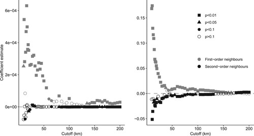
Overall, we find the results of the models for the distance cut-offs presented in Table 3 to be in line with the results obtained from models A, B and C (Table 2). The estimates for the area and population size are very close to those from the contiguity models, indicating the presence of an inverse density effect and that population size is associated with higher employment levels, respectively. Looking at a broader range of cut-offs (Figure 2),¹³ we find positive impacts of air connectivity on first-order neighbours (in line with the contiguity models) that decline rapidly over the first 60 km. In comparison, the shadow impacts on second-order neighbours are most dominant over the first 30 km (i.e., for regions that are no more than 30 km away from the airport). This suggests that airports’ positive impacts (linked to demand linkage and agglomeration spillover effects) can be found in close proximity to airports, whereas agglomeration shadow impacts are limited to immediate second-order neighbours. The positive effect of employment agglomeration declines more rapidly (more localized) due to more pronounced agglomeration shadow effects on immediate second-order neighbours; compared with connectivity, the second-order neighbours’ impacts become insignificant over longer distances.

As a robustness check, we drop the population and area controls (see Figures A10 and A11 in Appendix A in the supplemental data online). Similarly to Figure 2, the first-order lagged connectivity effects attenuate to zero before turning negative while remaining significant. The second-order effects are positive for short distances; the lagged employment effects oscillate between positive and negative. The irregularity of these spatial trends (cf. Figure 2) emphasizes the importance of normalizing a region’s size when quantifying spatial–economic impacts, possibly due to measurement problems associated with spatial units (Arbia, 1989). Our results are robust to including a year 2008 dummy to control for the 2008 financial crisis (see Figures A19 and 20 online). Next, we rerun our analysis with different subsets of instruments to check the validity and robustness of our instrumentation approach. Without instruments (see Figures A12 and A13 online), the first-order marginal effects of lagged connectivity retain their spatial trends but no longer attenuate to zero; the total effects are higher by one order of magnitude (compared with using all four instruments). These persistently higher positive effects are consistent with the expected positive bias of reverse causality. When used individually (see Figures A14 and A15 online), all four instruments show spatial trends and effect sizes similar to Figures 2 and 4.

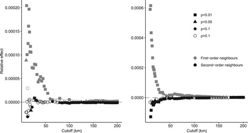
The attenuation impacts shown in Figure 2 suggests that both agglomeration of employment and access to air connectivity create localized positive impacts in close-by regions, but negative (agglomeration shadow) impacts further away. However, before accepting this interpretation, we rule out that these trends are an artefact of our model. By increasing the distance cut-off, the lagged variables cover an increasing number of regions; thus, the lagged variables increase as employment or connectivity are summed over more regions or airports, possibly depressing the scale of the coefficient. We analyse this potential artefact by conducting a post-estimation procedure that calculates relative effects (or pseudo-densities) as a 10% increase in either connectivity or lagged employment per lag area considered.¹⁴ These pseudo-densities are unaffected by the scale of the lagged variables and thus only capture agglomeration effects. As shown in Figure 3, the general result is robust to this procedure. As such, the iterated marginal effects of connectivity and lagged employment do show attenuation effects in agglomeration.

Figure 3. Relative effects from model D at the average per area (km²) for the first- and second-order lags in (left) connectivity and (right) employment.

Note: Iterated results for model D (equation 2) using the distance-based weights matrix specification (specification II from Figure 1). Cut-offs shown represent the border between first- and second-order neighbours. Relative effects calculated as the (absolute) increase in employment per NUTS-3 region following a 10% increase in density, using the formula: $0.10b_x\overline{x}/A$, where A represents the area, that is, $A=\pi \mathrm{cutof}{\mathrm{f}}^2$ for the first-order neighbours and $A=\pi (2\times \mathrm{cutoff}{)}^2-\pi \mathrm{cutof}{\mathrm{f}}^2$ for the second-order neighbours; and x represents the spatial lags in employment and connectivity.

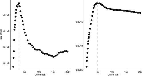
Given localized positive impacts on first-order neighbours and negative impacts on second-order neighbours, we compute the overall net effect of air connectivity and employment agglomeration on economic development (see Text A1 in the supplemental data online). These net effects, however, are calculated for models with different distance cut-offs. To control for differences in the spatial scope caused by varying the cut-off (i.e., at larger cut-off values, more regions are impacted), we calculate the average impact per impacted region. Figure 4 shows that the overall impacts of lagged connectivity and employment are positive for all model D variations with different distance cut-off values, which is in line with results from Campante and Yanagizawa-Drott (2018). This observation points towards overall positive economic development impacts of employment agglomeration and air connectivity, and hence not a zero-sum game. We find the captured total impacts to increase rapidly over the first 30 and 50 km for both air connectivity and lagged employment, respectively. This range is consistent with the results from estimating the marginal impact, which shows significant positive first-order neighbours’ impacts within these ranges. With further increases in the cut-off value, the first-order impacts (which act as a type of total effect by incorporating the second-order effect at smaller cut-offs) decline as more shadow impacts are considered.

Figure 4. Average total effect per impacted region from model D from a 1 unit increase in (left) connectivity and (right) employment.

Note: Iterated results for model D (equation 2) using the distance-based weights matrix specification (specification II from Figure 1). Cut-offs shown represent the border between first- and second-order neighbours.

We illustrate the implication of our results by calculating employment impacts of increasing air connectivity at an airport by 2200 points,¹⁵ which is equivalent to 5% of the year 2012 connectivity score of Brussels airport. As a case study, we consider two different areas: a 20-km radius (inner circle with 10 km radius and outer ring with 10 km width) and a 50-km radius (inner circle with 25 km radius and outer ring with 25 km width) (see Tables A9 and A10 in Appendix A in the supplemental data online). For the average NUTS-3 region, an increase in air connectivity by 2200 units considering a 20-km radius yields a summed impact of 193 additional service-sector jobs: 279 extra jobs due to connectivity increases in the first-order neighbours and 86 jobs lost due to a similar increase in connectivity in the second-order neighbours. For the average NUTS-3 region to experience the same increase in jobs (for the same radius considered), employment in the surrounding regions (neighbours) would need to increase by 2500 service-sector jobs: 210 extra jobs are gained due to employment increases in the first-order neighbours and 14 jobs are lost due to a similar increase in employment in the second-order neighbours. Looking at a radius of 50 km, an increase in air connectivity by 2200 units yields a summed impact of 298 additional service-sector jobs: 291 extra jobs due to improved air access nearby (the adverse impact from increasing connectivity far-away is near-zero for this cut-off level). For the average NUTS-3 region to experience the same increase in jobs, employment in the surrounding regions (neighbours) would need to increase by 36,000 service-sector jobs: 589 jobs are gained due to the increased access to employment nearby but also 296 jobs are lost due to the increased employment far-away. Since lagged connectivity and employment have different spatial allocations (connectivity being concentrated in small areas encompassing airports and employment being spread out over entire NUTS-3 regions), however, care should be taken when comparing their relative impacts.

DISCUSSION

Overall, our results imply positive employment impacts of air transport connectivity, which are concentrated in the vicinity of airports (below 30 km cut-off from airport). At the same time, second-order neighbours further away are negatively impacted by increases in connectivity (for maximum outer distances up to 60 km), which points towards the existence of agglomeration shadow effects at distances further away. By increasing the cut-off distance, the localized positive impacts of connectivity become mixed with the adverse shadow effects, which explains the reduction in the absolute value of both the positive first-order and adverse second-order marginal effects. In sum, these results provide evidence for a very localized nature of agglomeration economics. These localized impacts of aviation contrast with the much bigger catchment areas reported by Lieshout (2012), showing that demand patterns and economic impact patterns of airports are not necessarily interrelated. The spatial extent observed for the economic impacts follows previous findings at the commuting area (Patacchini & Zenou, 2007) and city level (Redding & Sturm, 2008) but is less localized than those observed by previous studies using postal codes (Duranton & Overman, 2005; Rosenthal & Strange, 2003) and more localized than previous studies at the provincial or county level (Hanson, 2005; Mion, 2004).

These findings have relevant implications for policymakers in their quest to develop regional airports. In recent years, many regional governments, which often act as airport shareholders or operators in Europe, have offered airlines incentives for route and traffic development (Allroggen et al., 2013; Malina et al., 2012; Núñez-Sánchez, 2015). One reason for granting these incentives is the perception that better air links cause a competitive advantage for a region, thereby creating jobs and income. Our results provide some support for this reasoning. Within the European Union, regional state aid for airports is only allowed if the aid is compatible with the internal market provisions; that is, state aid should be aimed at regional development or accessibility and should not distort the market or adversely affect trade within the European Union (European Commission, 2013). In practice, aid for operating, infrastructure investment or launching new routes must be temporary and restricted to small airports only. Recent examples from France regarding Béziers and Montpellier airports (European Commission, 2019a, 2020) show the difficulty of carefully balancing the trade-off between ensuring free airport competition on the one hand and regional competition for air connectivity and its resulting impacts on the other.

In light of the current legal framework in Europe, a relevant question for policymakers is whether regions indeed suffer a competitive disadvantage from having limited access to the air transport network. The present study provides two-fold evidence in that regard. First, the positive service sector employment effects, which would be in addition to potential direct effects of airport activity, are limited to a radius of approximately 60 km around the airport. Second, improvements in regional connectivity come at the expense of economic growth being diverted from other regions – with the net impact being positive, on average. The current legal framework does not explicitly weigh the positive and negative effects of improved air access, but including such thinking could avoid wasteful competition among European regions in attracting connectivity through state aid.

CONCLUSIONS

This study is the first to systemically quantify the wider economic impacts of aviation, including its spatial distribution, by applying the NEG and spatial–econometric models. We quantify the aggregate agglomeration and spillover effects and agglomeration shadow effects from access to air connectivity using NUTS-3 regions in Europe for the years 2001–12. For this purpose, we employ various spatial–econometric specifications for capturing proximity. Our spatial model of choice incorporates distance-based weight matrices, allowing us to iterate the cut-off distance and study agglomeration at a more refined geographical level and measure potential spatial attenuation effects over distance.

The results show air connectivity in first-order (nearby) neighbours to affect employment positively (agglomeration impacts) and in second-order (remote) neighbours to affect employment negatively (agglomeration shadow). The marginal effects of connectivity attenuate quickly for the first 60 km. The second-order air connectivity effects diminish to near-zero within the first 30 km – that is, for regions that are no more than 30 km away from the airport. As a result, the average total impact of connectivity is positive and peaks at a radius of around 30 km but declines quickly. Compared with airport catchment areas (Lieshout, 2012, p. 2), the impacts of air connectivity are more localized. Therefore, we show that airport catchment areas do not necessarily overlap with an airport’s economic impact area. The spatial extent of the agglomeration effects detected follows previous non-aviation studies on a similar regional level (Hanson, 2005; Mion, 2004; Patacchini & Zenou, 2007; Redding & Sturm, 2008) but are significantly more localized than in previous studies estimating agglomeration at the postal code level (Duranton & Overman, 2005; Rosenthal & Strange, 2003).

Our results are in line with recent evidence suggesting that improved air services can benefit core regions at the expense of peripheral regions with an overall positive impact (Campante & Yanagizawa-Drott, 2018). Our study improves upon existing work through (1) the application of a theoretically sound air connectivity index; (2) the use of an explicit spatial–econometric model with different specifications and aviation network-driven instruments; (3) the separate estimation of nearby and remote spatial effects as hypothesized by the NEG; and (4) the calculation of total effects for different cut-off distances, allowing a more refined overall impact estimation of air connectivity.

Our findings have important policy implications for regional airport development. They support the idea that regions without a local airport might suffer a competitive disadvantage since (1) airports only generate very localized positive impacts (peaking around a radius of 60 km); and (2) since access to airports is not ubiquitous, improvements in regional connectivity can result in (relative) disadvantages for other regions.

The major limitation of our study is that access to airports is proxied by distance. Further research should focus on exploring alternative measures of airport access like road travel time. Similarly, this study does not consider national borders, which might act as barriers to labour mobility, for example following Brexit. In the same vein, access to the airport might be a function of airport size and traffic offering if larger airports enjoy larger catchment areas. Another limitation of this study is the small set of control variables. Furthermore, we only calculate average spatial effects, and therefore, spatial heterogeneity (i.e., differential impacts between members of the European Union) is not considered (Chi, 2012). These expansions of our work are left for future research.

ACKNOWLEDGEMENTS

We thank Thomas de Graaff (VU Amsterdam) for valuable feedback on the empirical part of this paper. We also thank the participants at the conference of the International Transportation Economics Association (ITEA) 2019 for helpful discussions on earlier versions of this manuscript.

DISCLOSURE STATEMENT

No potential conflict of interest was reported by the authors.

Notes

1. Night lights are used as a proxy for economic activity.

2. Except for simultaneous lags in the dependent variable, independent variables and error terms.

3. Bold text represents matrices, italic text represents vectors and plain text refers to scalars.

4. Indicators that are impacted by both connectivity and employment acts as colliders and should not be controlled for (see Figure A3, panel B, in Appendix A in the supplemental data online).

5. From a technical point of view, even if the relationship between flight shares and connectivity were bidirectional, that would not cause the instrument to be endogenous. One counter-argument to the exogeneity of megacity shares is that abnormally high employment levels might be linked to activities of international organizations (such as the United Nations, including its specialized agencies: the World Bank, the Organization for Economic Co-operation and Development (OECD), European Communities, etc.) and activities of diplomatic and consular missions, which are concentrated in just a few cities and frequently interact, violating the exogeneity condition for the share of flights to megacities. However, given that this type of employment (level U from the NACE classification system) only makes up < 1% of the employment levels considered here at country level (see the fourth section) (Eurostat, 2021), the correlation between employment and megacity flight shares may not be substantial.

6. Note that X represents X_c here, but it can also represent weighted covariates if included.

7. We are interested in the catalytic impact of aviation as a driver of productivity growth and an attractor of economic activity. Therefore, we exclude employment derived from the construction and operation of airports and corresponding chain of suppliers of goods and services, and the employment generated by the spending of incomes by these employees.

8. The variables mentioned are area of intermodal transport at the airport (available for 89 out of 679 airports used in the analysis, ranging from 2003 to 2012) (Eurostat, 2022) and population accessible within 90 min by road and road transport performance (available for 1175 out of 1343 NUTS-3 regions used in the analysis, for 2016) (European Commission, 2019b). All three variables yield a correlation coefficient of less than 25% with air connectivity.

9. This restriction reduces noise in the allocation of the outer spatial weights matrices and results in sparse spatial weight matrices, leading to increased computational efficiency (Pace & Barry, 1997). Additionally, using distance permits correcting for border effects in connectivity by considering airports in European countries outside the European Union (see Figure A2 and Table A4 in Appendix A in the supplemental data online). Results are similar when the limit is set to √2 × cut-off (so both zones have equal area) and 4 × cut-off (see Figures A8 and A9 online).

10. The share-based weights used in model E also allow comparing the first- and second-order neighbouring lags as the weights are calculated similarly for both types of lags.

11. Without instrumentation, the impact of connectivity increases for model A and decreases for models B and C (see Table A7 in Appendix A in the supplemental data online).

12. Similarly, we find the contiguity-based first- and second-order impacts of employment to be negative. This result is unexpected and may also be driven by the artificial definition of NUTS-3 region borders. This effect is analysed further in the fifth section.

13. Due to their relative cut-off independence, the population and area effects and the model diagnostics (R², instrument validity tests) are not repeated for the broader range of cut-offs (Figure 2).

14. These impacts can be calculated as 0.10b_x $\overline{x}$/A, where b_x represents the coefficient estimates; A represents the area, that is, A = πcutoff² for the first-order neighbours and A = π(2 × cutoff)² – πcutoff² for the second-order neighbours; and x represents the spatial lags in employment or connectivity.

15. We assume the airport is located 10 and 25 km (precisely at the edge between the inner and outer neighbours), respectively, from the region under study so that both sets of neighbours experience in increase in connectivity of 1100 units.

REFERENCES

- Allroggen, F. (2013). Foerdert ein leistungsfaehiges Verkehrssystem die wirtschaftliche Entwicklung? Zeitschrift für Verkehrswissenschaft, 84(3), 2–43.
- Allroggen, F., & Malina, R. (2014). Do the regional growth effects of air transport differ among airports? Journal of Air Transport Management, 37, 1–4. https://doi.org/10.1016/j.jairtraman.2013.11.007
- Allroggen, F., Malina, R., & Lenz, A.-K. (2013). Which factors impact on the presence of incentives for route and traffic development? Econometric evidence from European airports. Transportation Research Part E: Logistics and Transportation Review, 60, 49–61. https://doi.org/10.1016/j.tre.2013.09.007
- Allroggen, F., Wittman, M. D., & Malina, R. (2015). How air transport connects the world–A new metric of air connectivity and its evolution between 1990 and 2012. Transportation Research Part E: Logistics and Transportation Review, 80, 184–201. https://doi.org/10.1016/j.tre.2015.06.001
- Andrews, D. W., & Stock, J. H. (2005). Identification and inference for econometric models: Essays in honor of Thomas Rothenberg. Cambridge University Press.
- Angrist, J. D., & Pischke, J.-S. (2008). Mostly harmless econometrics: An empiricist’s companion. Princeton University Press.
- Anselin, L., & Lozano-Gracia, N. (2008). Errors in variables and spatial effects in hedonic house price models of ambient air quality. Empirical Economics, 34(1), 5–34. https://doi.org/10.1007/s00181-007-0152-3
- Arbia, G. (1989). Spatial data configuration in statistical analysis of regional economics and related problems. Kluwer.
- Baltagi, B. (2005). Econometric analysis of panel data. Wiley.
- Blonigen, B. A., & Cristea, A. D. (2015). Air service and urban growth: Evidence from a quasi-natural policy experiment. Journal of Urban Economics, 86, 128–146. https://doi.org/10.1016/j.jue.2015.02.001
- Boschma, R. (2005). Proximity and innovation: A critical assessment. Regional Studies, 39(1), 61–74. https://doi.org/10.1080/0034340052000320887
- Brueckner, J. K. (2003). Airline traffic and urban economic development. Urban Studies, 40(8), 1455–1469. https://doi.org/10.1080/0042098032000094388
- Button, K., & Yuan, J. (2013). Airfreight transport and economic development: An examination of causality. Urban Studies, 50(2), 329–340. https://doi.org/10.1177/0042098012446999
- Campante, F., & Yanagizawa-Drott, D. (2018). Long-range growth: Economic development in the global network of air links. The Quarterly Journal of Economics, 133(3), 1395–1458. https://doi.org/10.1093/qje/qjx050
- Chi, G. (2012). The impacts of transport accessibility on population change across rural, suburban and urban areas: A case study of Wisconsin at sub-county levels. Urban Studies, 49(12), 2711–2731. https://doi.org/10.1177/0042098011431284
- Cidell, J. (2015). The role of major infrastructure in subregional economic development: An empirical study of airports and cities. Journal of Economic Geography, 15(6), 1125–1144. https://doi.org/10.1093/jeg/lbu029
- Combes, P.-P., & Gobillon, L. (2015). The empirics of agglomeration economies. In Duranton, G., Henderson, J. V., & Strange, W. C. (Eds.), Handbook of regional and urban economics (pp. 247–348). Elsevier.
- Combes, P.-P., & Overman, H. G. (2004). The spatial distribution of economic activities in the European Union. In Henderson, J. V. and Thisse, J.-F. (Eds.), Handbook of regional and urban economics (pp. 2845–2909). Elsevier.
- Dall’erba, S., & Le Gallo, J. (2008). Regional convergence and the impact of European structural funds over 1989–1999: A spatial econometric analysis. Papers in Regional Science, 87(2), 219–244. https://doi.org/10.1111/j.1435-5957.2008.00184.x
- Dekle, R., & Eaton, J. (1999). Agglomeration and land rents: Evidence from the prefectures. Journal of Urban Economics, 46(2), 200–214. https://doi.org/10.1006/juec.1998.2118
- Duranton, G., & Overman, H. G. (2005). Testing for localization using micro-geographic data. The Review of Economic Studies, 72(4), 1077–1106. https://doi.org/10.1111/0034-6527.00362
- Elhorst, J. P. (2010). Applied spatial econometrics: Raising the bar. Spatial Economic Analysis, 5(1), 9–28. https://doi.org/10.1080/17421770903541772
- Elhorst, J. P. (2014). Spatial econometrics: From cross-sectional data to spatial panels. Springer.
- European Commission. (2013). Guidelines on regional state aid for 2014–2020. Official Journal, C209, 23 July, 1–45.
- European Commission. (2019a). State aid: France to recover €8.5 million of illegal aid to Ryanair at Montpellier airport. https://ec.europa.eu/commission/presscorner/detail/en/IP_19_4991
- European Commission. (2019b). Road transport performance in Europe. https://ec.europa.eu/regional_policy/en/information/publications/working-papers/2019/road-transport-performance-in-europe
- European Commission. (2020). State aid: Commission opens in-depth investigation procedure into measures in favour of Béziers Airport in France and Ryanair. https://ec.europa.eu/commission/presscorner/detail/en/ip_20_366
- Eurostat. (2008). NACE Rev. 2 – Statistical classification of economic activities.
- Eurostat. (2021). National accounts employment data by industry (up to NACE A*64). http://appsso.eurostat.ec.europa.eu/nui/show.do?dataset=nama_10_a64_e
- Eurostat. (2022). Airport connections to other modes of transport. https://ec.europa.eu/eurostat/databrowser/view/AVIA_IF_ARP_CO/default/table?lang=en
- Eurostat GISCO. (2019). https://ec.europa.eu/eurostat/web/gisco/geodata
- Fageda, X. (2017). International air travel and FDI flows: Evidence from Barcelona. Journal of Regional Science, 57(5), 858–883. https://doi.org/10.1111/jors.12325
- Fageda, X., & Gonzalez-Aregall, M. (2017). Do all transport modes impact on industrial employment? Empirical evidence from the Spanish regions. Transport Policy, 55, 70–78. https://doi.org/10.1016/j.tranpol.2016.12.008
- Fageda, X., & Olivieri, C. (2019). Transport infrastructure and regional convergence: A spatial panel data approach. Papers in Regional Science, 98(4), 1609–1631. https://doi.org/10.1111/pirs.12433
- Fingleton, B., & Le Gallo, J. (2008). Estimating spatial models with endogenous variables, a spatial lag and spatially dependent disturbances: Finite sample properties. Papers in Regional Science, 87(3), 319–339. https://doi.org/10.1111/j.1435-5957.2008.00187.x
- Fujita, M., Krugman, P. R., & Venables, A. J. (1999). The spatial economy: Cities, regions and international trade. Wiley Online Library.
- Glaeser, E. L., & Kohlhase, J. E. (2004). Cities, regions and the decline of transport costs. Papers in Regional Science, 83(1), 197–228. https://doi.org/10.1007/s10110-003-0183-x
- González-Val, R. (2019). The spatial distribution of US cities. cities, 91, 157–164. https://doi.org/10.1016/j.cities.2018.11.015
- Green, R. K. (2007). Airports and economic development. Real Estate Economics, 35(1), 91–112. https://doi.org/10.1111/j.1540-6229.2007.00183.x
- Hanson, G. H. (2005). Market potential, increasing returns and geographic concentration. Journal of International Economics, 67(1), 1–24. https://doi.org/10.1016/j.jinteco.2004.09.008
- Head, K., & Mayer, T. (2004). The empirics of agglomeration and trade. In Henderson, J. V., & Thisse, J.-F. (Eds.), Handbook of regional and urban economics (pp. 2609–2669). Elsevier.
- Hodgson, C. (2018). The effect of transport infrastructure on the location of economic activity: Railroads and post offices in the American West. Journal of Urban Economics, 104, 59–76. https://doi.org/10.1016/j.jue.2018.01.005
- Holmes, T. J., & Stevens, J. J. (2004). Spatial distribution of economic activities in North America. In Henderson, J. V., & Thisse, J.-F. (Eds.), Handbook of regional and urban economics (pp. 2797–2843). Elsevier.
- Jaffe, A. B., Trajtenberg, M., & Henderson, R. (1993). Geographic localization of knowledge spillovers as evidenced by patent citations. The Quarterly Journal of Economics, 108(3), 577–598. https://doi.org/10.2307/2118401
- Kelejian, H. H., & Prucha, I. R. (1998). A generalized spatial two-stage least squares procedure for estimating a spatial autoregressive model with autoregressive disturbances. The Journal of Real Estate Finance and Economics, 17(1), 99–121. https://doi.org/10.1023/A:1007707430416
- Kelejian, H. H., & Prucha, I. R. (1999). A generalized moments estimator for the autoregressive parameter in a spatial model. International Economic Review, 40(2), 509–533. https://doi.org/10.1111/1468-2354.00027
- Kelejian, H. H., Prucha, I. R., & Yuzefovich, Y. (2004). Instrumental variable estimation of a spatial autoregressive model with autoregressive disturbances: Large and small sample results. Advances in Econometrics: Spatial and Spatio-Temporal Econometrics, 18, 163–198. https://doi.org/10.1016/S0731-9053(04)18005-5
- Knoben, J., & Oerlemans, L. A. (2006). Proximity and inter-organizational collaboration: A literature review. International Journal of Management Reviews, 8(2), 71–89. https://doi.org/10.1111/j.1468-2370.2006.00121.x
- Krugman, P. (1991). Increasing returns and economic geography. Journal of Political Economy, 99(3), 483–499. https://doi.org/10.1086/261763
- Lakew, P. A., & Bilotkach, V. (2018). Airport delays and metropolitan employment. Journal of Regional Science, 58(2), 424–450. https://doi.org/10.1111/jors.12369
- Lakshmanan, T. R. (2011). The broader economic consequences of transport infrastructure investments. Journal of Transport Geography, 19(1), 1–12. https://doi.org/10.1016/j.jtrangeo.2010.01.001
- Lenaerts, B., Allroggen, F., & Malina, R. (2021). The economic impact of aviation: A review on the role of market access. Journal of Air Transport Management, 91, 102000. https://doi.org/10.1016/j.jairtraman.2020.102000
- Lenaerts, B., Malina, R., & Allroggen, F. (2020). Measuring the quality of air transport networks. In Graham, A., Adler, N., Niemeier, H.-M., Betancor, O., Antunes, A. P., Bilotkach, V., Calderón, E. J., & Martini, G. (Eds.), Air transport and regional development policies (pp. 6–30). Routledge.
- LeSage, J. P. (2014). What regional scientists need to know about spatial econometrics.
- LeSage, J. P., & Pace, R. K. (2009). Introduction to spatial econometrics (statistics, textbooks and monographs). CRC Press.
- LeSage, J. P., & Pace, R. K. (2011). Pitfalls in higher order model extensions of basic spatial regression methodology. Review of Regional Studies, 41(1), 13–26. https://doi.org/10.52324/001c.8141
- Lieshout, R. (2012). Measuring the size of an airport’s catchment area. Journal of Transport Geography, 25, 27–34. https://doi.org/10.1016/j.jtrangeo.2012.07.004
- Malina, R., Albers, S., & Kroll, N. (2012). Airport incentive programmes: A European perspective. Transport Reviews, 32(4), 435–453. https://doi.org/10.1080/01441647.2012.684223
- Manski, C. F. (1993). Identification of endogenous social effects: The reflection problem. The Review of Economic Studies, 60(3), 531–542. https://doi.org/10.2307/2298123
- Mion, G. (2004). Spatial externalities and empirical analysis: The case of Italy. Journal of Urban Economics, 56(1), 97–118. https://doi.org/10.1016/j.jue.2004.03.004
- Núñez-Sánchez, R. (2015). Regional public support to airlines and airports: An unsolved puzzle. Transportation Research Part E: Logistics and Transportation Review, 76, 93–107. https://doi.org/10.1016/j.tre.2015.02.005
- Oak Ridge National Laboratory (ORNL). (2019). https://landscan.ornl.gov
- Pace, R. K., & Barry, R. (1997). Sparse spatial autoregressions. Statistics & Probability Letters, 33(3), 291–297. https://doi.org/10.1016/S0167-7152(96)00140-X
- Patacchini, E., & Zenou, Y. (2007). Spatial dependence in local unemployment rates. Journal of Economic Geography, 7(2), 169–191. https://doi.org/10.1093/jeg/lbm001
- Percoco, M. (2010). Airport activity and local development: Evidence from Italy. Urban Studies, 47(11), 2427–2443. https://doi.org/10.1177/0042098009357966
- Poelman, H. (2013). Measuring accessibility to passenger flights in Europe: Towards harmonised indicators at the regional level. Regional Focus, Brussels, Directorate-General for Regional and Urban Policy of the European Commission.
- Redding, S. J., & Rossi-Hansberg, E. A. (2017). Quantitative spatial economics. Annual Review of Economics, 9(1), 21–58. https://doi.org/10.1146/annurev-economics-063016-103713
- Redding, S. J., & Sturm, D. M. (2008). The costs of remoteness: Evidence from German division and reunification. American Economic Review, 98(5), 1766–1797. https://doi.org/10.1257/aer.98.5.1766
- Redding, S. J., & Turner, M. A. (2015). Transportation costs and the spatial organization of economic activity. In Duranton, G., Henderson, J. V., & Strange, W. C. (Eds.), Handbook of regional and urban economics (pp. 1339–1398). Elsevier.
- Redfearn, C. L. (2009). Persistence in urban form: The long-run durability of employment centers in metropolitan areas. Regional Science and Urban Economics, 39(2), 224–232. https://doi.org/10.1016/j.regsciurbeco.2008.09.002
- Rosenthal, S. S., & Strange, W. C. (2003). Geography, industrial organization, and agglomeration. Review of Economics and Statistics, 85(2), 377–393. https://doi.org/10.1162/003465303765299882
- Rosenthal, S. S., & Strange, W. C. (2004). Evidence on the nature and sources of agglomeration economies. In Henderson, J. V., & Thisse, J.-F. (Eds.), Handbook of regional and urban economics (pp. 2119–2171). Elsevier.
- Sanderson, E., & Windmeijer, F. (2016). A weak instrument F-test in linear IV models with multiple endogenous variables. Journal of Econometrics, 190(2), 212–221. https://doi.org/10.1016/j.jeconom.2015.06.004
- Serafini, R., & Ward, M. (2011). Chapter 10 exploring the determinants of employment in Europe: The role of services. In Tatsiramos, K., & Polachek, S. W. (Eds.), Research in labor economics (pp. 341–384). Emerald Group Publishing Limited.
- Sheard, N. (2019). Airport size and urban growth. Economica, 86(342), 300–335. https://doi.org/10.1111/ecca.12262