Estimating canopy height change using machine learning by coupling WorldView-2 stereo imagery with Landsat-7 data

ABSTRACT

Canopy height change (CHC) is one of the key characteristics of forest dynamics, associated with the fluctuations in forest above-ground biomass and carbon stocks. Field measurements and Airborne Laser Scanning (ALS) point clouds can be used to detect CHC; however, they have limited availability in space and time, making it challenging to map CHC over large areas. Alternatively, very high-resolution (VHR) satellite stereo imagery plays an increasingly vital role in estimating fine-scaled digital surface models (DSMs) across landscapes. However, its capability and potential to estimate canopy height model (CHM) and CHC has not been widely explored. Using ALS-derived CHM in 2011 and 2015 and the four-year CHC as references, we evaluated stereo-based CHM and CHC from WorldView-2 over five woody parks in Columbus, Ohio, USA. We also integrated stereo-based CHM with vegetation indices from Landsat 7 to improve CHM and CHC estimation with machine learning methods. Our results showed that VHR stereo imagery captured similar spatial patterns of CHM with ALS data but significantly overestimated CHM. Moreover, the ALS-derived CHC ranged from 1.6±1.9 m (mean ± standard deviation) to 3.1±1.2 m, as compared to from -1.3±0.7 m to 1.1±1.7 m for stereo-based CHC, indicating the limitation of CHC estimation by stereo imagery alone. Among six widely used machine learning methods, Gradient Boosting Regression method provided the most reliable estimates of CHM, with a correlation coefficient R of 0.64 and a root-mean-square error (RMSE) of 3.1 m (11.1%). Stereo-based CHM and vegetation indices explained more than 70% of CHM variability, substantially improving the estimation of 4-year CHC. Our results suggested that VHR stereo imagery alone has limitations in estimating CHM and CHC. The combination of remote-sensing structural (stereo-based CHM) and spectral (vegetation indices) information improves the CHM and CHC estimations.

KEYWORDS:

• canopy height change
• WorldView-2
• VHR stereo imagery
• Airborne Laser Scanning
• vegetation indices
• machine learning

1. Introduction

Canopy height change (CHC) is an essential indicator of forest dynamics, affecting forest structure, vegetation productivity, above-ground biomass, and carbon stocks over time (Lefsky 2010; Banin et al. 2012; Zhang et al. 2016). Traditionally, forest inventory programmes have collected tree height on sample plots and built age–height relationships to predict future height growth (Brosofske et al. 2014). However, plot-level canopy height measurements are sparse and unsuitable for spatially and temporally continuous observation. Thus, better representation of CHC is needed for sustainable management, such as estimating allowable cuts and detecting forest dynamics.

Over the last two decades, Light Detection And Ranging (LiDAR) has been widely adopted to measure vertical forest structure and related attributes such as volume and biomass (Nelson, Krabill, and Tonelli 1988). Airborne LiDAR or Airborne Laser Scanning (ALS) is capable of mapping forest structure at high spatial resolution, but their availability is limited in space and time. In contrast, spaceborne LiDAR data from ICESAT, ICESAT-2, and GEDI missions provide a global coverage to enable global mapping of canopy height model (CHM) (Lefsky 2010; Simard et al. 2011) but the spatial resolution of their wide-footprint (Abdalati et al. 2010) is insufficient for detailed forest management. Recently, stereo imagery from very high-resolution (VHR) satellites, such as GeoEye-1, WorldView-1, and WorldView-2, has become a cost-efficient alternative to ALS point clouds to generate digital surface model (DSM) (Saldaña et al. 2012; Shean et al. 2016; Zhou et al. 2015). High-resolution DSMs generated from VHR satellite stereo imagery have been used to study above-ground features in urban areas (EEckert and Hollands 2010; Tian, Cui, and Reinartz 2014), mountains (Toutin 2002; Zhang and Gruen 2006), forests (DeWitt et al. 2017), and grasslands (Hobi and Ginzler 2012). For forested landscapes, Tian et al. (2017) compared the performance of DSM estimation from multiple satellite stereo sensors (ALOS/PRISM, Cartosat-1, RapidEye, and WorldView-2), indicating the relative reliability of WorldView-2 in detecting forest structures. CHM can be directly created by subtracting digital terrain model (DTM) from DSM. There are a growing number of studies evaluating CHM derived from VHR satellite stereo imagery (CHM-S) (Persson and Perko 2016; St-Onge, Hu, and Vega 2008; Straub et al. 2013). For example, Straub et al. (2013) assessed Cartosat-1 and WorldView-2 stereo imagery for CHM and timber volume estimation, demonstrating the potential of satellite stereo imagery for regionalization of sample plot inventories. Persson and Perko (2016) assessed the CHM-S from WorldView-2 in boreal forests using aerial ALS-derived CHM (CHM-A) as a reference, with a root-mean-square error (RMSE) of 1.5 m (8.3%). However, WorldView-2 images alone could not accurately estimate CHM because it is influenced by vertical forest structure, the different viewing directions of the stereo pair, topography- and sun angle-based illumination, and vegetation phenology (leaf-on/off status) (Straub et al. 2013). Similarly, limitations of VHR stereo imagery in estimating CHM were reported in Australian tropical savannas (Goldbergs et al. 2019), caused by the wind-induced crown movement that affects stereo-pair point matching. Although forest DSM and CHM have been evaluated in previous studies (Persson and Perko 2016; Ullah et al. 2020), the capability of using multi-temporal VHR stereo imagery in detecting CHC has not yet been well studied and evaluated.

Trees grow towards brighter conditions (vertically) in a quest for light and simultaneously expand the crown to capture more of the available light (horizontally). Vegetation indices, such as the Normalized Difference Vegetation Index (NDVI) and the Enhanced Vegetation Index (EVI), can be used to detect vegetation greenness that is highly related to canopy horizontal expansion and height growth (Hyde et al., 2006). For example, a combination of ALS data and NDVI measurements improves the estimation of CHM and above-ground biomass compared to ALS or NDVI alone (Schaefer and Lamb 2016). Vegetation indices also help estimate canopy volume and above-ground biomass, suggesting the relationship between remote sensing spectral and structural metrics (Maimaitijiang et al. 2019). Given the potential limitation of VHR stereo imagery in estimating CHM accurately, the combination of stereo data and vegetation indices might be a better approach to detect CHC.

Machine learning methods have been widely used in CHM estimation. The typical machine learning task in all relevant studies is to learn a predictive model using potential predictors to predict the value of forest canopy height for unseen cases (Stojanova et al. 2010). Support Vector Machine has been used to improve the estimation of forest canopy attributes, such as CHM, basal area, and above-ground biomass, with the input of ALS composite metrics (Zhao et al. 2011). Similarly, Li et al. (2020) mapped high-resolution CHM using a deep learning method and random forest model by coupling ICESat-2 LiDAR with Sentinel-1, Sentinel-2, and Landsat-8 data. However, the performance of different machine learning methods in CHM estimation using stereo imagery has not been studied. The combination of stereo imagery-based structural information with vegetation indices-based spectral information provides the potential to improve CHM estimation and detect CHC accordingly. Thus, the main aim of this study is to build a machine learning-based CHM model for estimating CHC. To achieve this goal, we: (1) evaluated CHM-S derived from WorldView-2; (2) compared the performance of machine learning methods in estimating CHM and quantified the importance of predictors; (3) predicted and evaluated machine learning-based CHM and CHC.

2. Methods and materials

2.1. Study area

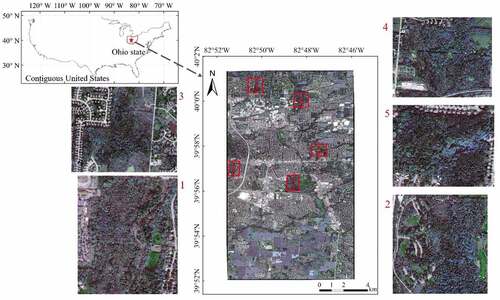
Our study area is located in eastern Columbus (39.521–40.013°N, 82.459–82.515°W), Ohio, U.S.A. (Figure 1), covering approximately 145 km² over five woody parks, including Big Walnut Park, Blacklick Woods Metro Park, Gahanna Woods Park, Olde Quarry Park, and Pine Quarry Park. Pine Quarry Park is mainly covered by pine trees, such as pitch pine (Pinus rigida) and Virginia pine/scrub pine (Pinus virginiana). The other four parks are covered by deciduous broadleaf and mixed forests, mainly composed of American beech (Fagus grandifolia), sugar maple (Acer saccharum), and oak and hickory species of trees, such as chestnut oak (Quercus montana) and pignut hickory (Carya glabra). The terrain is relatively flat, ranging from 230 m to 300 m above sea level. The annual mean temperature is 11.5ºC, and total precipitation is 1016 mm, with an average count of rainfall of 130 days per year (https://www.noaa.gov/). We collected data and developed and tested methods for these five parks in this study.

Figure 1. Study areas in eastern Columbus, Ohio, U.S.A, including five woody parks (image: WorldView-2, October 8th, 2011). Park1–5 are Big Walnut Park, Blacklick Woods Metro Park, Gahanna Woods Park, Olde Quarry Park, and Pine Quarry Park, respectively.

2.2. Data

2.2.1. ALS point clouds data

ALS data were obtained from the Ohio Statewide Imagery Program (OSIP), which aims to provide high-resolution imagery for the State of Ohio and to support the geospatial needs of government service providers and Geographic Information System users (https://ogrip.oit.ohio.gov/ProjectsInitiatives/OSIPDataDownloadsLiDAR.aspx). For this study, ALS data were acquired in March 2011 and April 2015 using a Leica ALS70 (lidar) system on board a Woolpert aircraft. The detailed specifications of the ALS data are summarized in Table 1. Multiple returns were recorded for each laser pulse, along with an intensity value for each return. The point density is nearly 25 points/m². The point cloud was classified to determine bare-earth and non-ground points.

Table 1. ALS flight parameters.

Parameters	Description
Flying speed (km/h)	150
Flying height (ft)	6500
Field of view (degree)	40
Pulse rate (kHz)	272
Scan rate (Hz)	41
Average side lap (%)	25

2.2.2. VHR stereo satellite imagery

VHR stereo imageries were acquired from WorldView-2, a commercial satellite from Maxar launched in October 2009 with high resolution and eight bands (https://www.maxar.com/). The detailed specification of stereo imageries is listed in Table 2. For this study, we used stereo data in 2011 and 2015 to match the ALS data acquisition years. Stereo data were acquired in October 2011 and September 2015. It should be noted that the acquisition time of ALS data and VHR stereo data were not consistent, which might bring the uncertainty of CHM and CHC estimation.

Table 2. WorldView-2 satellite parameters.

Parameters	Description
Orbit altitude (km)	770
Sensor bands	8
Sensor resolution (m)	Panchromatic: 0.46; Multispectral: 1.85
Swath width (km)	16.4
Revisit frequency (day)	1m GSD: 1.1; 20 degrees off-nadir: 3.7
Max Contiguous Area Collected in a Single Pass (km)	Mono: 138*112 (8 strips); Stereo: 63*112 (4 pairs)

2.2.3. Satellite vegetation indices

In this study, we used the open-access Landsat 7 reflectance datasets (16-day, 30 m) to calculate vegetation indices, including Normalized Difference Vegetation Index (NDVI) and Enhanced Vegetation Index (EVI). NDVI and EVI can be calculated as follows:

(1) $\mathrm{N}\mathrm{D}\mathrm{V}\mathrm{I}=\frac{{\rho }_{\mathrm{N}\mathrm{I}\mathrm{R}}-{\rho }_{\mathrm{R}\mathrm{E}\mathrm{D}}}{{\rho }_{\mathrm{N}\mathrm{I}\mathrm{R}}+{\rho }_{\mathrm{R}\mathrm{E}\mathrm{D}}}$(1)

(2) $\frac{\mathrm{E}\mathrm{V}\mathrm{I}=2.5{\rho }_{\mathrm{N}\mathrm{I}\mathrm{R}}-{\rho }_{\mathrm{R}\mathrm{E}\mathrm{D}}}{{\rho }_{\mathrm{N}\mathrm{I}\mathrm{R}}+6{\rho }_{\mathrm{R}\mathrm{E}\mathrm{D}}-7.5{\rho }_{BLUE}+1}$(2)

where ${\rho }_{\mathrm{N}\mathrm{I}\mathrm{R}}$, ${\rho }_{\mathrm{R}\mathrm{E}\mathrm{D}}$, ${\rho }_{\mathrm{B}\mathrm{L}\mathrm{U}\mathrm{E}}$ is the reflectance of near-infrared, red, and blue, respectively. Here, we used the Google Earth Engine (GEE), a cloud platform to obtain and process free-archived satellite data, to process and download the Landsat 7 data (Tian et al. 2022). We calculated the average NDVI and EVI during the growing season (March–September) in 2011 and 2015 as the satellite-based spectral information. One of the main goals of our study was to explore the potential of open-access satellite data in predicting canopy height and height change. Thus, we used Landsat 7 spectral bands to generate NDVI and EVI as covariates for our machine learning models in this study.

2.3. CHM extraction from ALS point clouds and VHR stereo satellite imagery

We applied the LiDAR360 V4.0, a comprehensive point cloud post-processing software (https://greenvalleyintl.com), to conduct ALS point clouds data processing. Before generating DTM, we removed noise points using the functions of Remove Outliers and Noise Filter. Here, we applied the triangulated irregular network (TIN) as an interpolation method and used ground return to generate DTM (0.5 m, consistent with VHR stereo data). Then, we used first-return points to generate DSM, and raw CHM-A was obtained by subtracting DTM from DSM (Figure 2).

Figure 2. The methodological workflow of this study. DSM, DTM, CHM, and CHC are digital surface model, digital terrain model, canopy height model, and canopy height change, respectively. NDVI and EVI are Normalized Difference Vegetation Index and Enhanced Vegetation Index, respectively. SVR, RFR, BR, GBR, DTR, and ETR are Support Vector Regression, Random Forest Regression, Bagging Regression, Gradient Boosting Regression, Decision Tree Regression, and Extra-Trees Regression, respectively.

We used the rational polynomial coefficient (RPC) stereo processor (RSP) software to generate DSM from VHR stereo imagery (Qin 2016). The RSP can generate level 2 rectification, geo-referencing, point cloud generation, pan-sharpen, DSM resampling, and ortho-rectification (Figure 2). This software applies a hierarchical semi-global matching method as the current matching strategy. The SGM method is based on the idea of pixelwise matching of Mutual Information and approximating a global, 2D smoothness constraint by combining many 1D constraints. The SGM also applies a multi-path dynamic programming to optimize the cost function (Hirschmüller 2008). The final DSM from VHR stereo data has a spatial resolution of 0.5 m. The CHM-S was generated by subtracting ALS-derived DTM from stereo-derived DSM.

2.4. Machine learning methods of CHM prediction and accuracy assessment

We applied and compared six widely used machine learning methods to estimate CHM, including Support Vector Regression, Random Forest Regression, Bagging Regression, Gradient Boosting Regression, Decision Tree Regression, and Extra-Trees Regression (Li et al. 2020; Stojanova et al. 2010; Tian, Nielsen, and Reinartz 2014; Zhao et al. 2011). All machine learning methods were conducted with Python3.7.4 using the ‘SciKit Learn’ library. These machine learning methods can be categorized into four types, i.e. Supervised Learning Method, Averaging Ensemble Method, Boosting Ensemble Method, and Non-parametric Supervised Learning Method (Table 3). For each model, predictor variables include CHM-S and vegetation indices (NDVI and EVI). CHM-A was used as reference data for training and validation. Given the spatial resolution of vegetation indices were 30 m, we resampled CHM-A and CHM-S into 30 m using the bilinear interpolation method. After removing ground and low vegetation such as grasses and shrubs (CHM <3 m), we collected a total of 1856 available pixels (30 × 30 m) for five parks in 2011, among which 80% of pixels were randomly selected as the training dataset, and the remaining 20% pixels were used as the test dataset. We applied the Z-score normalization method to normalize all predictor variables for training and testing (Figure 2). During the tuning of each model, we used 5-fold cross-validation, evaluated by the RMSE, to avoid overfitting and to get optimal parameters. During the cross-validation processes, the training data set was divided into five equal parts. The first part was kept as the testing set and the remaining four parts are used to train the model. Then the trained model was evaluated on the testing set.

Table 3. Comparison of different machine learning methods of estimating CHM.

Machine Learning methods	Type	R	RMSE (m)	Execution time (s)
Support Vector Regression (SVR)	Supervised Learning Method	0.087	6.611	2.377
Random Forest Regression (RFR)	Averaging Ensemble Method	0.603	3.294	29.445
Bagging Regression (BR)	Averaging Ensemble Method	0.386	4.571	1.586
Gradient Boosting Regression (GBR)	Boosting Ensemble Method	0.635	3.121	2.048
Decision Tree Regression (DTR)	Non-parametric Supervised Learning Method	0.168	8.499	0.229
Extra-Trees Regression (ETR)	Non-parametric Supervised Learning Method	0.151	8.287	0.182

We evaluated the performance of six different machine methods by RMSE, Pearson correlation coefficient (R), and model execution time. After the model selection, we determined the final model and applied it to estimate CHM for 2015 and 4-year CHC (2011–2015). The ALS-derived CHC (i.e. CHM-A₂₀₁₅ minus CHM-A₂₀₁₁) was used as reference data to validate predicted CHC (Figure 2) in terms of R and RMSE.

3. Results

3.1. Comparison of CHM and CHC from ALS point clouds and VHR stereo data

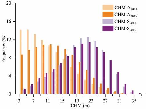
CHM-A and CHM-S, to some degree, showed similar spatial patterns, and the CHM of densely wooded areas was higher than the CHM covered by low plants. VHR stereo imagery data delineated large and clustered grasslands/bare grounds but missed some small canopy gaps with a smoother profile (Figure 3). Based on the histogram of CHM distribution (Figure 4), we found VHR stereo imagery significantly overestimated CHM in all parks. A higher frequency of middle to high CHM-A (10–30 m) was observed in 2015 compared to 2011, but no distinct pattern was found in CHM-S.

Figure 3. Comparison of CHM derived from ALS point clouds and VHR stereo data for a densely woody area in Pine Quarry Park. The aerial photo (a) and NDVI (d) was derived from VHR satellite imagery. (b) and (c) are the CHM derived from ALS point clouds for 2011 and 2015, respectively. (e) and (f) are the CHM derived from VHR stereo imagery for 2011 and 2015, respectively.

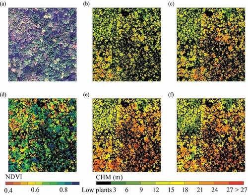
Figure 4. Histogram of CHM derived from ALS point clouds and VHR stereo imagery for all parks combined in 2011 and 2015.

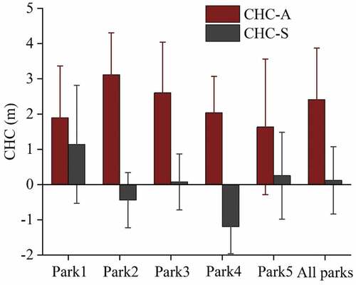
Taking Pine Quarry Park as an example, we found a considerable divergence between CHC-A and CHC-S in terms of spatial distribution (Figure 5a,b) and frequency (Figure 5c). More than half of CHC-S ranged from 0 to 2 m, leading to a lower average CHC compared to CHC-A (0.3 ± 1.6 m vs. 1.6 ± 1.1 m). CHC-S was significantly correlated with CHC-A, with an R of 0.15 (p = 0.041) and an RMSE of 4.84 m (24.2%) (Figure 5d). With regard to all parks, we found consistent underestimations of CHC for stereo data. The range of CHC-A among five parks is from 1.6 ± 1.9 m (mean ± standard deviation) to 3.1 ± 1.2 m, but it decreased to −1.3 ± 0.7 m to 1.1 ± 1.7 m for CHC-S (Figure 6).

Figure 5. Comparison of CHC derived from ALS point clouds (CHC-A) and stereo data (CHC-S) for Pine Quarry Park. (a) and (b) are the spatial distribution of CHC-A and CHC-S, respectively. (c) is the frequency of CHC-A and CHC-S. (d) is the relationship between CHC-A and CHC-S.

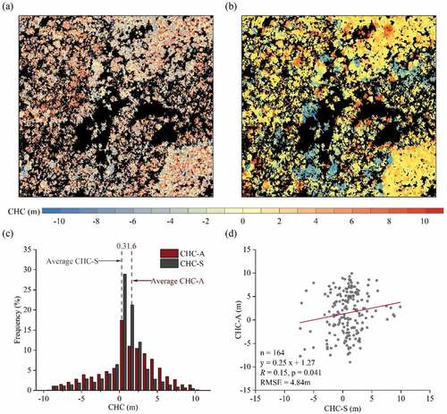
Figure 6. Comparison of CHC-A and CHC-S for all parks. Park1–5 are Big Walnut Park, Blacklick Woods Metro Park, Gahanna Woods Park, Olde Quarry Park, and Pine Quarry Park, respectively. The bars indicate mean ± standard deviation.

3.2. Comparison of CHM prediction using different machine learning methods

Six different machine learning methods generated a large discrepancy in CHM prediction in 2011 (Table 3). Regarding R and RMSE, RFR (R: 0.603, RMSE: 3.294 m) and GBR (R: 0.635, RMSE: 3.121 m) showed comparatively better performance predicting CHM than the remaining methods. Meanwhile, we found that the execution time of RFR was much longer than that of GBR, with a value of 29.445 s and 2.048 s, respectively. By utilizing the feature importance tool, we obtained sorted feature importance (Figure 7): CHM-S (0.43), EVI (0.21), and NDVI (0.14).

Figure 7. Sorted feature importance of the CHM prediction using GBR.

3.3. Validation of machine learning-based CHC

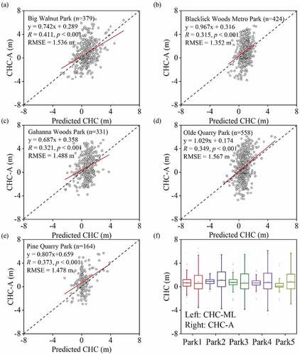
Among CHCs predicted by the machine learning method (i.e. GBR) for five parks, the lowest RMSE (1.352 m) was found in Blacklick Woods Metro Park, and the highest RMSE was observed in Olde Quarry Park (1.567 m). Significant correlations were identified between CHC-A and predicted CHC (p < 0.001), with R of 0.411 for Big Walnut Park, 0.315 for Blacklick Woods Metro Park, 0.321 for Gahanna Woods Park, 0.349 for Olde Quarry Park, and 0.373 for Pine Quarry Park, respectively (Figure 8a-e). For each park, the mean value of predicted CHC was close to the mean values of CHC-A, but the latter was more dispersed than the former (Figure 8F), indicating underestimated spatial variability in predicted CHC.

Figure 8. Validation of machine learning-based CHC. (a)-(e) are the correlations between CHC-A and predicted CHC for five parks. (f) is the distribution of CHC-A and predicted CHC.

4. Discussion

Although the performance of VHR stereo imagery for the retrieval of CHM has not been studied intensively, several studies point out the limitations of CHM estimation using solely WorldView-2 stereo imagery (Straub et al. 2013; Aguilar et al. 2014; Immitzer et al. 2016; Persson and Perko 2016; Goldbergs et al. 2019). Consistently, our results showed that the dense image matching technique for WorldView-2 stereo imagery captures CHM spatial patterns but severely overestimates CHM (Figure 4). Apart from the constraints of the stereo matching technique, there are several related reasons that result in the poor estimation of CHM. For example, the acquisition time of ALS point clouds (April, which is close to the start of the growing season) is different from that of WorldView-2 stereo data (September, towards the end of the growing season). Vegetation phenological indicators, such as leaf on and leaf off, partially explained the variability of CHM (Solvin, Puliti, and Steffenrem 2020). In addition, stereo matching underestimates canopy gap sizes and numbers, leading to continuous canopies and shrinking grasslands and bare grounds (Figure 3). Potential crown movement (e.g. caused by wind) also affects stereo-pair point matching (Straub et al. 2013). Regarding CHC, we found that stereo imagery alone cannot provide robust detection of CHC, with a substantial underestimation (Figure 6). The main reason for poor estimation of CHC by stereo imagery is due to the uncertainty of CHM estimation and objects continuity. Specifically, the dense matching methods for stereo imagery pose a continuity constraint to have the estimated height in favour of spatially continuous measurements to avoid the surface being too noisy. Therefore, dense matching is limited to capturing and retaining the vertical information for non-continuous canopy, leading to considerable uncertainty in CHM and CHC (Ullah et al. 2020). Thus, poor estimations of CHM and CHC reduce the application of VHR stereo imagery in estimating canopy height and its change.

By integrating canopy structural (CHM-S) and spectral (NDVI and EVI) information, we compared six widely used machine learning methods for estimating CHM. Our results showed that CHM estimated by the ensemble method (Boosting and Averaging) is more accurate than other machine learning methods. Even though RFR has been widely used in CHM estimation (Ahmed et al. 2015; Li et al. 2020), we found that other machine learning methods are computationally much more efficient than RFR, due to the relatively high n_estimators in the RFR model (Chen et al. 2019; Li and Xie 2018). Among six machine learning methods, GBR is the most reliable method for estimating CHM in terms of R and RMSE. Interestingly, we found that the feature importance of EVI is higher than NDVI (0.21 vs. 0.14, Figure 7), suggesting that, for dense canopy, EVI can better represent canopy spectral information compared to NDVI that is apt to become saturated in densely vegetated areas.

Regarding the limitations of this study, one of the potential reasons for the overestimation of CHM-S is the mismatch of acquisition time for ALS point clouds and WorldView-2 data related to canopy leaf-on/off status. This leads to uncertainty in the evaluation of CHM-S. Although the mismatch of data acquisition time between ALS and VHR is not ideal, our study is unique in its comparison of ALS and stereo VHR in two different years (most current studies only focused on the comparison of ALS and stereo VHR in a single year). Moreover, the leaf on/off conditions in two years (SP2015-SP2011 for ALS and AU2015-AU2011 for stereo VHR) are similar, which allows both ALS and stereo data to estimate canopy height change over four years. Another mismatch is the spatial resolution of different datasets, which also undermines the reliability of methods in this study. Given that CHM-A is affected by the high transmissivity of ALS points, better gap-filling methods and field data are needed in the future to improve model reliability.

5. Conclusions

In this study, we evaluated the performance of WorldView-2 stereo imagery in estimating CHM and CHC in five woody parks. We found that stereo imagery matching alone overestimated CHM and underestimated four-year CHC. By coupling CHM-S and vegetation indices, we compared six machine learning methods for estimating CHM and finally built a GBR-based CHM model. CHM-S, NDVI, and EVI explained >70% variability of CHM. The final CHM model showed an accurate estimation of CHC in terms of the mean value for each park, with an RMSE range of 1.352–1.567 m, but underestimates the spatial variability of CHC. This study illustrates that by integrating CHM derived from WorldView-2 stereo imagery and satellite vegetation indices, we provide a new machine learning-based approach to detect CHC, which can help monitor forest changes in above-ground biomass, vegetation productivity, and carbon storage even in large scales.

Acknowledgements

We acknowledge the Ohio Statewide Imagery Program for providing ALS data.

Disclosure statement

No potential conflict of interest was reported by the authors.

References

- Abdalati, W., H. J. Zwally, R. Bindschadler, B. Csatho, S. L. Farrell, H. A. Fricker, D. Harding, et al. (2010). The ICESat-2 Laser Altimetry Mission. Proceedings of the IEEE, 98, 735–751.
- Aguilar, M. A., M. Del Mar Saldaña, F. J. Aguilar, and A. G. Lorca. 2014. “Comparing Geometric and Radiometric Information from GeoEye-1 and WorldView-2 Multispectral Imagery.” European Journal of Remote Sensing 47: 717–738. doi:10.5721/EuJRS20144741.
- Ahmed, O. S., S. E. Franklin, M. A. Wulder, and J. C. White. 2015. “Characterizing Stand-Level Forest Canopy Cover and Height Using Landsat Time Series, Samples of Airborne LiDar, and the Random Forest Algorithm.” Isprs Journal of Photogrammetry and Remote Sensing 101: 89–101. doi:10.1016/j.isprsjprs.2014.11.007.
- Banin, L., R. Feldpausch, O. L. Phillips, T. R. Baker, J. Lloyd, K. Affum-Baffoe, E. J. M. M. Arets, et al. 2012. “What Controls Tropical Forest Architecture? Testing Environmental, Structural and Floristic Drivers.” Global Ecology and Biogeography 21 (12): 1179–1190. doi:10.1111/j.1466-8238.2012.00778.x.
- Brosofske, K. D., R. E. Froese, M. J. Falkowski, and A. Banskota. 2014. “A Review of Methods for Mapping and Prediction of Inventory Attributes for Operational Forest Management.” Forest Science 60 (4): 733–756. doi:10.5849/forsci.12-134.
- Chen, Y., W. Shen, S. Gao, K. Zhang, J. Wang, and N. Huang. 2019. “Estimating Deciduous Broadleaf Forest Gross Primary Productivity by Remote Sensing Data Using a Random Forest Regression Model.” Journal of Applied Remote Sensing 13 (3): 038502. doi:10.1117/1.JRS.13.038502.
- DeWitt, J. D., T. A. Warner, P. G. Chirico, and S. E. Bergstresser. 2017. “Creating High-Resolution Bare-Earth Digital Elevation Models (DEMs) from Stereo Imagery in an Area of Densely Vegetated Deciduous Forest Using Combinations of Procedures Designed for Lidar Point Cloud Filtering.” GIScience & Remote Sensing 54: 552–572. doi:10.1080/15481603.2017.1295514.
- Eckert, S., and T. Hollands. 2010. “Comparison of Automatic DSM Generation Modules by Processing IKONOS Stereo Data of an Urban Area.” IEEE Journal of Selected Topics in Applied Earth Observations and Remote Sensing 3 (2): 162–167. doi:10.1109/JSTARS.2010.2047096.
- Goldbergs, G., S. W. Mainer, S. R. Levick, and A. Edwards. 2019. “Limitations of High Resolution Satellite Stereo Imagery for Estimating Canopy Height in Australian Tropical Savannas.” International Journal of Applied Earth Observation and Geoinformation 75: 83–95. doi:10.1016/j.jag.2018.10.021.
- Hirschmüller, H. 2008. “Stereo Processing by Semiglobal Matching and Mutual Information.” IEEE Transactions on Pattern Analysis and Machine Intelligence 30 (2): 328–341. doi:10.1109/TPAMI.2007.1166.
- Hobi, M. L., and C. Ginzler. 2012. “Accuracy Assessment of Digital Surface Models Based on WorldView-2 and ADS80 Stereo Remote Sensing Data.” Sensors 12: 6347–6368. doi:10.3390/s120506347.
- Hyde, P., R. Dubayah, W. Walker, J. B. Blair, M. Hofton, and C. Hunsaker. 2006. “Mapping Forest Structure for Wildlife Habitat Analysis Using Multi-Sensor (LiDar, SAR/InSar, ETM+, Quickbird) Synergy.” Remote sensing of environment 102 (1–2): 63–73. doi:10.1016/j.rse.2006.01.021.
- Immitzer, M., C. Stepper, S. Böck, C. Straub, and C. Atzberger. 2016. “Use of WorldView-2 Stereo Imagery and National Forest Inventory Data for Wall-To-Wall Mapping of Growing Stock.” Forest Ecology and Management 359: 232–246. doi:10.1016/j.foreco.2015.10.018.
- Lefsky, M. A. 2010. “A Global Forest Canopy Height Map from the Moderate Resolution Imaging Spectroradiometer and the Geoscience Laser Altimeter System.” Geophysical Research Letters 37: L15401. doi:10.1029/2010GL043622.
- Li, W., Z. Niu, R. Shang, Y. Qin, L. Wang, and H. Chen. 2020. “High-Resolution Mapping of Forest Canopy Height Using Machine Learning by Coupling ICESat-2 LiDar with Sentinel-1, Sentinel-2 and Landsat-8 Data.” International Journal of Applied Earth Observation and Geoinformation 92: 102163. doi:10.1016/j.jag.2020.102163.
- Li, Y., A. Hyder, L. T. Southerland, G. Hammond, A. Porr, and H. J. Miller. 2020. “311 Service Requests as Indicators of Neighborhood Distress and Opioid Use Disorder.” Scientific reports 10: 19579. doi:10.1038/s41598-020-76685-z.
- Li, Y., and Y. Xie. 2018. “A New Urban Typology Model Adapting Data Mining Analytics to Examine Dominant Trajectories of Neighborhood Change: A Case of Metro Detroit.” Annals of the American Association of Geographers 108 (5): 1313–1337. doi:10.1080/24694452.2018.1433016.
- Maimaitijiang, M., V. Sagan, P. Sidike, M. Maimaitiyiming, S. Hartling, K. T. Peterson, M. J. W. Michael Maw, N. Shakoor, T. Mockler, and F. B. Fritschi. 2019. “Vegetation Index Weighted Canopy Volume Model (CVMVI) for Soybean Biomass Estimation from Unmanned Aerial System-Based RGB Imagery.” Isprs Journal of Photogrammetry and Remote Sensing 151: 27–41. doi:10.1016/j.isprsjprs.2019.03.003.
- Nelson, R., W. Krabill, and J. Tonelli. 1988. “Estimating Forest Biomass and Volume Using Airborne Laser Data.” Remote Sensing of Environment 24: 247–267. doi:10.1016/0034-4257(88)90028-4.
- Persson, H. J., and R. Perko. 2016. “Assessment of Boreal Forest Height from WorldView-2 Satellite Stereo Images.” Remote Sensing Letters 7: 1150–1159. doi:10.1080/2150704X.2016.1219424.
- Qin, R. 2016. “Rpc Stereo Processor (Rsp) – a Software Package for Digital Surface Model and Orthophoto Generation from Satellite Stereo Imagery.” ISPRS Annals Photogrammetry, Remote Sensing and Spatial Information Science III-1: 77–82. doi:10.5194/isprs-annals-III-1-77-2016.
- Saldaña, M. M., M. A. Aguilar, F. J. Aguilar, and I. Fernández. 2012. “DSM Extraction and Evaluation from GeoEye-1 Stereo Imagery.” XXII Congress of the International Society for Photogrammetry and Remote Sensing I-4: 113–118. doi:10.5194/isprsannals-I-4-113-2012.
- Schaefer, M. T., and D. W. Lamb. 2016. “A Combination of Plant NDVI and LiDar Measurements Improve the Estimation of Pasture Biomass in Tall Fescue (Festuca Arundinacea Var. Fletcher).” Remote Sensing 8 (2): 109. doi:10.3390/rs8020109.
- Shean, D. E., O. Alexandrov, Z. M. Moratto, B. E. Smith, I. R. Joughin, C. Porter, and P. Morin. 2016. “An Automated, Open-Source Pipeline for Mass Production of Digital Elevation Models (DEMs) from Very-High-Resolution Commercial Stereo Satellite Imagery.” Isprs Journal of Photogrammetry and Remote Sensing 116: 101–117. doi:10.1016/j.isprsjprs.2016.03.012.
- Simard, M., N. Pinto, J. B. Fisher, and A. Baccini. 2011. “Mapping Forest Canopy Height Globally with Spaceborne Lidar.” Journal of Geophysical Research: Biogeosciences 116: G04021. doi:10.1029/2011JG001708.
- Solvin, T. M., S. Puliti, and A. Steffenrem. 2020. “Use of UAV Photogrammetric Data in Forest Genetic Trials: Measuring Tree Height, Growth, and Phenology in Norway Spruce (Picea Abies L. Karst.).” Scandinavian Journal of Forest Research 35 (7): 322–333. doi:10.1080/02827581.2020.1806350.
- St-Onge, B., Y. Hu, and C. Vega. 2008. “Mapping the Height and Above-Ground Biomass of a Mixed Forest Using Lidar and Stereo Ikonos Images.” International Journal of Remote Sensing 29 (5): 1277–1294. doi:10.1080/01431160701736505.
- Stojanova, D., P. Panov, V. Gjorgjioski, A. Kobler, and S. Džeroski. 2010. “Estimating Vegetation Height and Canopy Cover from Remotely Sensed Data with Machine Learning.” Ecological informatics 5 (4): 255–256. doi:10.1016/j.ecoinf.2010.03.004.
- Straub, C., J. Tian, R. Seitz, and P. Reinartz. 2013. “Assessment of Cartosat-1 and WorldView-2 Stereo Imagery in Combination with a LiDar-DTM for Timber Volume Estimation in a Highly Structured Forest in Germany.” Forestry 86: 463–473. doi:10.1093/forestry/cpt017.
- Tian, H., T. Chen, Q. Li, Q. Mei, S. Wang, M. Yang, Y. Wang, and Y. Qin. 2022. “A Novel Spectral Index for Automatic Canola Mapping by Using Sentinel-2 Imagery.” Remote Sensing 14: 1113. doi:10.3390/rs14051113.
- Tian, J., S. Cui, and P. Reinartz. 2014. “Building Change Detection Based on Satellite Stereo Imagery and Digital Surface Models.” IEEE Transactions on Geoscience and Remote Sensing 52: 406–417. doi:10.1109/TGRS.2013.2240692.
- Tian, J., A. A. Nielsen, and P. Reinartz. 2014. “Improving Change Detection in Forest Areas Based on Stereo Panchromatic Imagery Using Kernel MNF.” IEEE Transactions on Geoscience and Remote Sensing 52: 7130–7139. doi:10.1109/TGRS.2014.2308012.
- Tian, J., T. Schneider, C. Straub, F. Kugler, and P. Reinartz. 2017. “Exploring Digital Surface Models from Nine Different Sensors for Forest Monitoring and Change Detection.” Remote Sensing 9: 287. doi:10.3390/rs9030287.
- Toutin, T. 2002. “Three-Dimensional Topographic Mapping with ASTER Stereo Data in Rugged Topography.” IEEE Transactions on Geoscience and Remote Sensing 40: 2241–2247. doi:10.1109/TGRS.2002.802878.
- Ullah, S., M. Dees, P. Datta, P. Adler, T. Saeed, M. S. Khan, and B. Koch. 2020. “Comparing the Potential of Stereo Aerial Photographs, Stereo Very High-Resolution Satellite Images, and TanDem-X for Estimating Forest Height.” International Journal of Remote Sensing 41 (18): 6976–6992. doi:10.1080/01431161.2020.1752414.
- Zhang, J., S. E. Nielsen, L. Mao, S. Chen, J. C. Svenning, and M. McGlone. 2016. “Regional and Historical Factors Supplement Current Climate in Shaping Global Forest Canopy Height.” The Journal of Ecology 104 (2): 469–478. doi:10.1111/1365-2745.12510.
- Zhang, L., and A. Gruen. 2006. “Multi-Image Matching for DSM Generation from IKONOS Imagery.” Isprs Journal of Photogrammetry and Remote Sensing 60 (3): 195–211. doi:10.1016/j.isprsjprs.2006.01.001.
- Zhao, K., S. Popescu, X. Meng, Y. Pang, and M. Agca. 2011. “Characterizing Forest Canopy Structure with Lidar Composite Metrics and Machine Learning.” Remote Sensing of Environment 115 (8): 1978–1996. doi:10.1016/j.rse.2011.04.001.
- Zhou, Y., B. Parsons, J. R. Elliott, I. Barisin, and R. T. Walker. 2015. “Assessing the Ability of Pleiades Stereo Imagery to Determine Height Changes in Earthquakes: A Case Study for the El Mayor-Cucapah Epicentral Area.” Journal of Geophysical Research: Solid Earth 120 (12): 8793–8808. doi:10.1002/2015JB012358.