Incorporating the effect of weather in construction scheduling and management with sine wave curves: application in the United Kingdom

Abstract

The impact of (adverse) weather is a common cause of delays, legal claims and economic losses in construction projects. Research has recently been carried out aimed at incorporating the effect of weather in project planning; but these studies have focussed on either a narrow set of weather variables, or a very limited range of construction activities or projects. A method for processing a country’s historical weather data into a set of weather delay maps for some representative standard construction activities is proposed. Namely, sine curves are used to associate daily combinations of weather variables to delay and provide coefficients for expected productivity losses. A complete case study comprising the construction of these maps and the associated sine waves for the UK is presented along with an example of their use in building construction planning. Findings of this study indicate that UK weather extends project durations by an average of 21%. However, using climatological data derived from weather observations when planning could lead to average reductions in project durations of 16%, with proportional reductions in indirect and overhead costs.

Keywords:

• Weather
• climate
• construction
• schedule
• project delay

Introduction

Many construction projects fail to meet their initially planned completion dates. This is a common phenomenon in many countries and affects almost all kinds of construction works (Alaghbari et al. 2007, Mahamid et al. 2012, Gündüz et al. 2013, Ruqaishi and Bashir 2015).

Lateness (understanding ‘late’ as missing the originally agreed completion date between the contractor and the project owner) has repercussions for almost all stakeholders (Thorpe and Karan 2008). From the public or private project owner’s perspective, late delivery of a project means delaying the start of an asset’s operation. This in turn might mean missing a business opportunity, losing a competitive advantage, delaying a return on investment, and ultimately reducing profits (Trauner et al. 2009, Głuszak and Les¨niak 2015). From the contractors’ perspective, late completion might involve contractual penalties and also blocks reallocation of resources for longer periods, limits the resources’ productive capacity, and generally increases the contractor’s indirect and overhead costs (Jang et al. 2008, Hamzah et al. 2011). From the subcontractors’ perspective, late projects generally make resource planning suboptimal as projections for resource demand are inaccurate and thus it is more likely that resource overlaps between multiple projects will occur (Shahin et al. 2011). From the end users’ perspective, late delivery of projects almost always causes some discomfort and disappointment, particularly if users live nearby and/or are affected by the construction works (Mezher and Tawil 1998).

In some cases, lateness can have certain positive outcomes. For example, activity costs can be reduced to some extent when a longer time span allows for more efficient allocation of resources. However, the benefits of these ‘intentional’ delays are almost entirely realized by the contractors, and other stakeholders merely experience the negative outcomes.

Among common causes of project delays, weather is consistently rated as one of the most frequent and harmful (Assaf and Al-Hejji 2006, AlSehaimi and Koskela 2008, Orangi et al. 2011, Mentis 2015). Weather can impact construction projects in multiple ways: by decreasing productivity and sometimes halting construction (Rogalska et al. 2006); by ruining unprotected and exposed constructed elements (El-Rayes and Moselhi 2001), by disrupting communications and/or blocking access to site locations (Alarcón et al. 2005), to cite but a few. Moreover, weather-related claims are a frequent source of dispute between contractors and project owners (Moselhi and El-Rayes 2002, Nguyen et al. 2010). It is not unusual that in the absence of agreement, unsettled claims can escalate into legal disputes and protracted litigation causing suspension of work for a longer period than the original abnormal weather episode itself (e.g. Finke 1990, Kumaraswamy 1997, Yogeswaran et al. 1998).

When categorizing the impact of weather, it is common to differentiate between foreseeable and unforeseeable weather (Tian and De Wilde 2011), as well as extreme and non-extreme (but generally combined) weather events (Jung et al. 2016).

Foreseeable weather is generally considered to encompass extreme adverse weather events that can impact the execution or exploitation of infrastructure unless precautionary measures are taken. Taking account of foreseeable weather is more frequently practised during the construction phase of special projects such as long, exposed bridges or high-rise buildings (Tanijiri et al. 1997, Jung et al. 2016). These types of projects normally have large budgets, and thus they are more likely to have resources for monitoring how and when on-site weather will cause changes to scheduled activities. Developments in sub-seasonal and seasonal weather forecasting have shown early promise too, but forecasts of acceptable quality still just span a maximum 10-d window (White et al. 2017).

However, despite advances in forecasting, there will always be an inherent uncertainty in a chaotic system such as the weather, which makes it difficult to always provide accurate forecasts. This is particularly true when considering extremes related to climate change (Sato et al. 2017).

Furthermore, whilst there are some construction activities that require forecast information for making good short-term decisions (e.g. whether to pour concrete today or tomorrow, or whether high winds will prevent work in exposed environments or at height), most resource-related operational decisions, and certainly all project planning, have to be undertaken anticipating weather beyond what current forecasting methods can predict. People (workers) have high manoeuvrability, but generally not the equipment, machinery, vehicles and special supplies that they employ. This is why this piece of research considers the applicability of climatology data drawn from historical weather information as opposed to simple weather forecasts. This does not mean, however, that the importance of relevant and sometimes crucial short-term weather forecasting is not acknowledged.

The main aim of this paper is to propose a new approach for processing historical weather information from a construction-relevant perspective. Combinations of weather variables and intensities that affect the execution of construction activities have been analyzed and processed into a series of maps for construction managers.

From now on, this paper is structured as follows: the Literature review section includes an overview of the most relevant pieces of research proposing models of the interaction between weather and construction productivity. The Materials and methods section provides a comprehensive step-by-step description of the method proposed. Namely, in this section, the proposed model is first outlined; then how all the necessary weather data were extracted and processed; and, finally, how most weather variability can be captured by and reduced to sine wave curves. Next, the Case study section describes the application of the proposed method to the construction of a reinforced concrete building in the UK. The Discussion section provides further analyses and insights for both the case study considered and alternative potential applications. The Conclusions section summarises and highlights the contributions of this paper to both the scientific community and the construction practitioners. Finally, the Supplemental online material contains all the calculations, weather maps (the main research outputs generated in this study), as well as some programmable spreadsheets that allow performing weather-aware project scheduling calculations.

Literature review

General meteorological and climate research covering forecasting or retrospective analysis is significant and will not be reviewed here. Instead, the focus will be on two main areas. The first comprises the most recent models that have integrated the effect of weather in the planning and/or execution of construction works. The second is the particular combinations of weather variables and intensities that can produce significant impacts with regard to the execution of representative and frequent construction activities.

Overview of weather models for construction projects

Research on how weather impacts the execution of construction projects is plentiful. However, only recently have quantitative models been developed for measuring the degree to which weather phenomena can cause a productivity decrease. A comprehensive sample of these quantitative models is summarized in Table 1.

Table 1. Sample of relevant research papers on the effect of weather on construction projects.

Project type	Publication year	Reference	Weather data source	Forecastingmodel	Activities analyzed	Weather agents
Buildings	1999	Thomas et al. (1999)	Historical (past) data	No	Steel structure delivery and erection activities	Temperature and snow
	2008	Jang et al. (2008)	Short-term (live) forecasts	Yes	Generic	Temperature and precipitation
	2008	Thorpe and Karan (2008)	Historical (past) data	No	Clearing and grubbing, excavation, foundations, structural erection, floors, interiors, roofs and HVAC	Temperature, snow, humidity and precipitation
	2010	David et al. (2010)	Historical (past) data	Yes	Generic	Solar radiation, temperature, humidity, wind
	2013	Dytczak et al. (2013)	Historical (past) data	No	Generic	Temperature and wind
	2013	Marzouk and Hamdy (2013)	Historical (past) data	Yes	Formwork	Precipitation and temperature
	2014	Shan and Goodrum (2014)	Historical (past) data	Yes	Steel structure	Temperature and humidity
	2014	González et al. (2014)	Historical (past) data	No	RC structures and finishing’s (e.g. partition walls, windows, and doors)	Not specified
	2016	Jung et al. (2016)	Historical (past) data	Yes	Generic + core wall, steel frame, deck plate, RC, curtain wall	Solar radiation, temperature, wind and precipitation
	2016	Li et al. (2016)	Historical (past) data	No	Steel reinforced bars	(Hot) temperature
	2017	Ballesteros-Pérez et al. (2017a, 2017b)	Historical (past) data	Yes	Earthworks, formworks, concrete, steelworks, scaffolding, outdoor paintings and asphalt pavements	Temperature, precipitation, wind and electrical storms
Highways	2001	El-Rayes and Moselhi (2001)	Historical (past) data	Yes	Earthworks, base courses, drainage layers and paving	Precipitation
	2010	Apipattanavis et al. (2010)	Historical (past) data	Yes	Concrete and asphalt paving, structures, excavations and grading	Precipitation, air and soil temperature and wind
	2013	Chinowsky et al. (2013)	Historical (past) data	Yes	Generic	Temperature and precipitation
Pipelines	2011	Shahin et al. (2011)	Historical (past) data	Yes	Clearing and grading, trenching, bedding, pipe-fusing, laying-in, hydro testing, compaction and backfilling	Air and soil temperature, wind, humidity and precipitation
	2012	Duffy et al. (2012)	Historical (past) data	Yes	Grading, stringing, bending, welding, trenching, coating, backfill, clean-up	Temperature, wind, and precipitation
Tunnelling	2014	Shahin et al. (2014)	Historical (past) data	Yes	All tunnelling process, hoisting and muck car cleaning	Air and soil temperature and wind
Bridges	2015	Ballesteros-Pérez et al. (2015)	Historical (past) data	Yes	Earthworks, formworks, concrete and asphalt pavements	Temperature, precipitation, wind and electrical storms

Table 1 is first organized by type of construction project (first column) and second by chronological order of publication (second column). It can clearly be seen that almost all works have been published in the last 10 years, and that building projects in particular have attracted the most attention. Furthermore, only one work proposes a forecasting model that uses live weather data retrieved from nearby stations to inform decisions regarding which construction activities to undertake in the short term. The remainder of the works containing forecasting models simply employs historical weather data. This suggests that there is a belief among construction researchers (or perhaps a lack of multidisciplinary input) that historical weather at nearby locations will be probabilistically or deterministically repeated to some extent in subsequent years. It is also a common practice to use synthetically generated weather series for informing management decisions.

However, it is necessary to point out that Table 1 only includes studies with construction-oriented forecasting models. As mentioned previously, forecasting models in pure meteorology and other applied fields have not been considered here. The impact of weather on each field of application can help to identify the relevant weather variables, and ultimately demonstrates the value of better forecasting. Most construction projects, however, generally involve many disparate activities each of which is susceptible to different combinations of weather variables and intensities.

To date, most studies have focussed on very narrow sets of activities (last but one column in Table 1) and/or have considered a limited number of weather variables (last column). This generally constitutes a necessary simplification due to the difficulty of obtaining local (representative) data for a sufficient number of weather variables and from a sufficient number of locations. Moreover, the data available must also be sufficiently consistent (not much data missing), fine-grained (daily, hourly) and from a sufficient number of previous years to be useful.

The method proposed later can be considered a continuation of Ballesteros-Pérez et al.’s (2015, 2017b) research. As can be seen in Table 1, their models have already been adapted to two different types of projects (buildings and bridges), and have considered a varied and representative set of activities common to many construction projects (earthworks, formworks, concrete, steelworks, scaffolding, outdoor paintings and asphalt pavements). These models are of particular interest because they are two of the few covering extensive geographical areas (almost the whole of Chile and Spain, respectively), which means they can be used as general country-wide planning tools by governments and contractors alike.

However, the proposed method extends the scope of previous research in this area. Most previous studies (including those of Ballesteros-Pérez et al.) have required the use of either probabilistic or time series curves with many parameters or points. Some have also been developed to work with long series of discrete registers for modelling local weather. In contrast, the method proposed here only requires simple sine wave curves with only one, two or three parameters depending on the level of accuracy required. This is a significant advantage as the simplicity of the developed expressions means most construction managers will easily be able to use them in practice, with hardly any mathematical expertise.

In the next section, the selection of weather variables considered in this study will be justified as well as their relationship with a representative set of cross-project construction activities.

Combinations of weather variables affecting construction activities

The weather involves the confluence of multiple phenomena (wind, rain, heat, etc.) that quite often do not involve a clear correlation of occurrence with each other (Ballesteros-Pérez et al. 2017b). Studies analysing the seasonal variability of combinations of weather agents are quite scarce (Kim and Augenbroe 2012). However, it is precisely this weather variability (seasonal or not) that makes anticipating how weather will affect construction work difficult.

In this study, it is assumed that the impact of weather can be represented in a project schedule via activity duration extensions and, in some cases cost increases, and that weather-aware construction schedules can be useful tools for helping construction managers make better decisions.

The first stage is thus deciding which combinations of weather variables and intensities determine whether certain construction activities can be performed. The impact of a particular set of weather variables and intensities on an activity can be very different depending on the: construction technologies employed, equipment used, materials involved and/or procedures adopted; how exposed the construction site is; how persistently (consistently and/or repetitively) the weather is classed as unusual; what is considered the average (or normal) weather in the particular region (or country). However, it is still possible to choose a combination of weather variables that, under some common conditions (e.g. same country, similar construction technologies, materials and construction practices), can be considered as ‘relatively representative’ of the regional/industry standard. This study will consider the thresholds for the weather variables described in Table 2 as precluding the stated construction activities.

Table 2. Weather variables and thresholds assumed to cause non-working days.

Weather variable (daily value)	Earthworks (E)	Concrete (C)	Formworks/scaffolding (F)	Steelworks (S)	Outdoor paintings (O)	Asphalt pavements (P)
Minimum temperature ≤0 °C		×				×
Mean temperature ≤0 °C	×			×	×
Maximum temperature ≥40 °C		×		×		×
Precipitation ≥1 mm					×	×
Precipitation ≥10 mm	×	×
Precipitation ≥30 mm				×
Hail precipitation					×	×
Snow precipitation					×	×
Electrical storm			×	×
Wind gusts ≥30 knots		×	×	×	×

As noted, the combination of weather variables in Table 2 might not be appropriate for many countries or contexts. However, it is considered sufficiently representative for the UK which is where the proposed method will be applied later. Similar combinations of weather variables have also been considered recently by other authors (Ballesteros-Pérez et al. 2017a, 2017b) for both Spain and the UK.

By way of explanation for the values chosen, earthwork activities are more difficult to execute when the ground is partially or totally frozen (Shahin et al. 2011, 2014) or when too much water causes a slope to become partially unstable (NCHRP 1978, El-Rayes and Moselhi 2001).

Concerning activities involving concrete, the minimum temperature must not drop below 0 °C before it has hardened, otherwise it will microfracture (American Concrete Institute 1985). The temperature must also not rise above 40 °C and/or the wind speed exceed 30 knots, or the concrete will dry out too fast when curing (American Concrete Institute 1985). In addition, the amount of extra water coming from rain, snow or hail must be small (e.g. 10 mm), otherwise the water/cement ratio will vary affecting the concrete’s final strength and durability (NCHRP 1978, American Concrete Institute 1985).

Formwork and Scaffolding activities are affected in a similar manner by the weather. In particular, their execution is unsafe during electrical storms (due to the risk of electrocution) (Rogalska et al. 2006) and high winds (Nguyen et al. 2010, Marzouk and Hamdy 2013).

Steelwork activities are also sensitive to electrical storms and high winds (Irizarry et al. 2005), but in addition are affected by extremely high and low temperatures (Thomas et al. 1999) and excessive amounts of rain (particularly welding) (Thorpe and Karan 2008).

Outdoor painting activities can be difficult to execute when it is raining, snowing or hailing as when the paint is still fresh, extra water can decrease the effectiveness of the primer and/or lead to colour changes (Ballesteros-Pérez et al. 2015). Water-based paints can also lose their adherence if they freeze when drying. In addition, painting in windy areas is risky as painting equipment, like buckets, can be blown over or fall onto lower levels (Nguyen et al. 2010).

Finally, asphalt pavements are very susceptible to the addition of small quantities of water (in the form of rain, snow or hail) (El-Rayes and Moselhi 2001, Apipattanavis et al. 2010), and to extremely high and low temperatures (NCHRP 1978).

Materials and methods

Method outline

This section will describe a method for processing historical weather information from a construction-relevant perspective. The weather data employed is limited to inland stations, because the latter normally register more weather variables than at sea. The method involves three main stages.

The first stage involves gathering and analysing historical daily weather data from as many weather stations as possible. By ‘analysing’, we mean calculating the percentage of each day considered ‘workable’ in previous years, where workable implies that none of the weather variables exceeded the threshold values in Table 2 such that the completion of an activity would be prevented. More specifically, the analysis involves calculating percentages of workable days for every single day of the year (1–365), for each of the six construction activities [e.g. earthworks (E), concrete (C), formworks/scaffolding (F), steelworks (S), outdoor paintings (O) and asphalt pavements (P)].

The second stage involves fitting sine wave curves to the data for the percentage of workable days for all days of the year. Each type of activity and weather station require one sine wave curve, and then all of the parameters from the various sine wave curves for a particular activity can be represented on contour maps. These maps allow easy interpolation of the values of the sine wave parameters for a particular site when no weather stations are located nearby.

Finally, the third stage involves applying the necessary location-specific sine wave data to a construction schedule so that time (and cost) extensions can be anticipated. In this latter stage, it will be assumed, as in almost all previous models, that past weather and climate patterns will be repeated to some extent in the upcoming years for a given location.

The next two subsections include detailed descriptions of the first and second stages, respectively. The following section (Case study) will describe stage three, i.e. the application of the weather model to a project schedule.

Analysis of UK weather data

This subsection will detail and exemplify how calculation of the number of workable days was performed for the UK (England, Wales, Scotland and Northern Ireland) for the six generic types of construction activities described in Table 2.

First, daily weather data were retrieved from the UK Met Office (2018) databases, particularly from the MIDAS dataset. Data were extracted from only those weather stations with daily registers of maximum, minimum and mean temperature, rainfall and maximum wind gust, as well as snow, hail and thunder flags. Additionally, only weather stations that started registering these variables between 1986 and 1996 were selected for the sake of representativeness. Thirty years are the standard adopted by the World Meteorological Organization for analysing climatic patterns. However, we resorted to a minimum of 20 years coverage to increase the number of stations from 40 to 102, and because Vose and Menne (2004) proved that 20 years were quite likely to be beyond what is necessary for capturing interannual variability for construction works. In any case, even departing with 20–30 years nominally, in most cases, the meteorological equipment at each station had either malfunctioned and/or required periodic maintenance resulting in blank periods in the data.

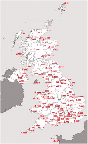
Therefore, 102 stations were eventually considered from across the UK spanning 20–30 years, but with occasional (normally minor) data blank periods. The locations of these stations are shown in Figure 1 where they are marked using the UK Met Office (2018) codes from the MIDAS dataset.

Figure 1. Locations of weather stations used for the analysis.

It is worth highlighting that whenever at least one weather variable was not registered for a given day, that day was completely ruled out for that weather station. The reason for this was to avoid optimistic bias when assessing whether the day was workable (a day is more likely to be workable when fewer variables that might cause a day to be non-workable are considered).

The final cutoff criterion was whether the data from a given weather station for a particular type of construction activity had at least three complete registers for a given day (all weather variables registered) for at least half of the days (not necessarily consecutive) of the year. This filter ruled out two complete weather station registers from the initial 102, but also up to 48% of the weather stations for outdoor painting and asphalt pavement activities.

Nevertheless, with a minimum of 52 stations’ historical registers per activity, there was a considerable amount of data to be processed. The number of weather stations included was much larger than in most of the studies listed in Table 1, and generally many more complete years of data (around 23 on average per weather station) were analyzed. Complete calculations are available on the first Supplemental Online Material spreadsheet file for all stations and activity types.

The next step involved calculating the climatic reduction coefficients (CRC). A CRC, as defined by Ballesteros-Pérez et al. (2015), represents the percentage of each day in past years that was considered workable. This means that none of the relevant weather variables exceeded their threshold values from Table 2 for a given activity and weather station. Hence, the value of the CRC corresponds to the percentage, or per-unit value, representing the probability of a day being workable for a particular type of activity. A representative sample of CRC calculations for different weather stations and activity types (E, C, F, S, O and P) is shown in Figure 2. All CRC values can be found by activity type for all weather stations in the last six tabs of the same Supplemental Online Material spreadsheet.

Figure 2. Examples of average daily CRC calculations for all construction activities.

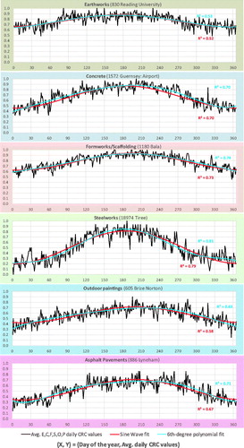
Along with the CRC data (black lines) in Figure 2, two smooth curve fits are shown: a sixth-degree polynomial (seven parameters) in blue, and a sine wave curve (up to three parameters) in red. As can be seen, both curves fit the data similarly, meaning the sine wave curve represents a good fit with the CRC data even with substantially fewer parameters. Later, the loss of precision after having resorted to sine wave expressions will also be examined.

Reduction of weather variability to sine waves

As exemplified in Figure 2, sine wave expressions were fitted to all weather stations’ CRC data for all types of construction activities. Sine waves, in this case, are mathematical expressions whose equations and parameters are of the form: (1) $$y=\text{CRC}=K+A·\text{cos}\left(\text{2pf}\left(x/\text{365}-\phi \right)\right)$$(1) where:

CRC: climatic reduction coefficients: (E, C, F, S, O and P). Percentage of workable days for each day of the year (x).

x: day of the year (days 1–365). In leap years, the 29th February is considered as x = 59.5.

K: vertical shift (in per unit). Approximately corresponds to the geometric mean of the annual CRC values.

A: amplitude (in per unit). Approximately corresponds to the maximum positive and negative average oscillation of the CRC values with respect to K.

f: frequency. This was set at 1 so that 365 d corresponded to one complete oscillation.

φ: phase shift (in per unit). Corresponds to the day of the year (but expressed in per unit) when the sine wave reaches its maximum value (optimum weather conditions). This is true because expression (1) has been built using a cosine, instead of a sine. However, unless multiple waves are compared, cosine waves are also named sine waves. We will follow the same terminology here and refer to expression (1) as a sine wave then.

Hence, each sine wave curve has three free parameters (K, A and φ). The values of these parameters were obtained by minimizing the least squares between each sine wave curve and its respective CRC data for each CRC data series (i.e. for each weather station and construction activity type).

A summary of the final (K, A and φ) parameter values can be found on the second tab of the Supplemental Online Material spreadsheet mentioned above. Details of the errors associated with the sine wave expressions can be found in the first tab of the same file. Errors between the CRC and the sixth-degree polynomial fits are also available for the cases where there were enough data.

However, a series of K, A and φ values are not necessarily immediately useful unless the construction site is geographically close to one of the weather stations. Therefore, a series of maps for each sine wave parameter and type of activity was developed. An example set of maps for the three parameters (K, A, and φ) corresponding to formworks/scaffolding activities is shown in Figure 3.

Figure 3. Example maps for vertical shift K (bottom), amplitude A (middle) and phase shift φ (top) for formworks/scaffolding activities in the UK.

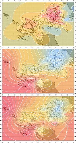
These contour maps were created with Surfer v.14^® (Golden software, CO, USA) from gridded data by implementing a Kriging interpolation method. This interpolation method was invented in the 1950s by the South African geologist Danie G. Krige for predicting distribution of minerals. However, it was mathematically formalized by the French engineer Georges Matheron in the 1960s (Matheron 1969). For statisticians, the Kriging interpolation method is also known as Gaussian process regression. This as it is a method of interpolation for which the interpolated values are modelled by a Gaussian process governed by prior co-variances. With only mild conditions on the priors, Kriging interpolation gives the best linear unbiased prediction of intermediate values, which is why this method was used here. Maps for the other five activities are included in the PDF file in the Supplemental Online Material.

Furthermore, one of the main aims of this study was to develop a series of expressions that were not just as representative as possible, but also as simple as possible. Therefore, after obtaining the original K, A and φ values for all weather stations and type of activity, the values were represented by type of construction activity graphically as shown in Figure 4. The intention was to determine whether the amplitude A and/or the phase shift φ could be expressed as a function of the vertical shift K in order to reduce the number of parameters in Equation (1)(1) $$y=\text{CRC}=K+A·\text{cos}\left(\text{2pf}\left(x/\text{365}-\phi \right)\right)$$(1) and obtain the simplest expressions possible.

Figure 4. Plots of K, A and φ values with regression expressions assumed.

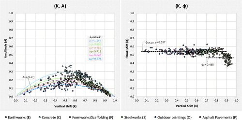
Quite surprisingly, the amplitude A exhibited a degree of correlation with K. This is probably due to some common boundary conditions for the two parameters. For example, when K has its lowest (K = 0) or highest (K = 1) value, A must equal zero (A = 0) as there is no oscillation possible. Similarly, A is expected to approach its maximum value when K is approximately equal to 0.5. Overall, this means that a single-parameter quadratic expression crossing the points (K = 0, A = 0) and (K = 1, A = 0) should model the correlation between the two variables. That quadratic expression corresponds to A = a_i(K – K²), and the best-fit values for a_i for the six types of activities are represented on the left hand of Figure 4.

In contrast, there was little correlation between K and φ; this was because φ does not vary significantly with K or the station location. This can be checked easily as the value of φ lies within a relatively narrow vertical band. Hence, it is possible to assume with little error, that φ is a constant for each type of activity. The two values of this constant (for earthworks and for all other activities) are given on the right side of Figure 4.

To summarise, the original three-parameter (3-p) sine wave expression can be reduced most of the time to a 2-p, or even a 1-p expression, by assuming that K is the only free parameter. In other words, A can be replaced by a quadratic expression which is a function of K (A = a_i(K – K²)) and φ can be assumed to be constant.

The remaining step involves checking whether the 3-p, 2-p and 1-p sine wave approximations generate sufficiently small errors in comparison to the original CRC data series. Details of the calculations can be found at the bottom of the second tab in the Supplemental Online Material spreadsheet and are summarized in Table 3.

Table 3. Errors in CRC estimates.

Data	Error	E	C	F	S	O	P	Average
3-p sine waves (K, A and φ are free)	MSE	0.004	0.017	0.012	0.016	0.017	0.017	0.01
	MAE	0.050	0.076	0.083	0.095	0.096	0.097	0.08
	MAPE	0.058	0.140	0.124	0.148	0.276	0.261	0.17
2-p sine waves (K and A are free, φ = constant)	MSE	0.005	0.010	0.013	0.017	0.017	0.017	0.01
	MAE	0.051	0.077	0.084	0.096	0.097	0.098	0.08
	MAPE	0.058	0.143	0.126	0.150	0.278	0.263	0.17
1-p sine waves (K free, A = f(K) and φ = constant)	MSE	0.005	0.010	0.013	0.017	0.018	0.018	0.01
	MAE	0.052	0.080	0.086	0.098	0.100	0.100	0.09
	MAPE	0.059	0.146	0.128	0.151	0.285	0.268	0.17
Deviations between neighbour data points (consecutive CRC values)	MSE	0.006	0.012	0.018	0.023	0.023	0.024	0.02
	MAE	0.057	0.084	0.098	0.108	0.112	0.114	0.10
	MAPE	0.067	0.168	0.157	0.184	0.337	0.322	0.21

Table 3 contains the mean squared errors (MSE), mean absolute errors (MAE) and mean absolute percentage errors (MAPE) for the three sine wave approximations for each type of construction activity. It also includes the average squared, absolute and percentage deviations between neighbour CRC points from consecutive days which reflects the small scale variability or jaggedness of the CRC curves. It can not only be seen from the data in Table 3 that the errors for the 2-p and 1-p sine waves are not significantly larger than the errors for the 3-p versions, but also that the errors remain below the deviations between neighbour points. This means that the simplified 2-p and 1-p sine waves closely reflect the CRC curves almost all of the time, and are not too dissimilar to the 3-p sine waves.

Finally, from the average R² values from all weather stations by type of construction activity (see the Excel spreadsheet with summary of all regression calculations in the Supplemental Online material), it can be claimed that overall, the proposed sine waves capture between 28% (at worst, for earthworks) and 79% (at best, for concrete) of the average weather variability, and this is accomplished with reasonably simple mathematical expressions suitable for use by construction managers during project planning. The final stage is to implement the developed expressions in a real project, which is the purpose of the next section.

Case study

An example of how the sine waves can be used during construction scheduling is contained in this section. The schedule proposed here represents the construction of a fictitious simplified three-storey reinforced concrete building. It consists of 24 activities arranged under three work packages, as shown in Figure 5.

Figure 5. Construction schedule for a simplified three-storey reinforced concrete building.

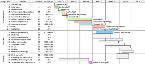
Figure 5 represents a weather-unaware schedule, or a schedule in which the activity durations have been calculated without considering the potential impact of the weather. The schedule represented in Figure 5, like the following schedules calculated later, has all been generated assuming unlimited resources. The way this weather-unaware schedule can be transformed into a weather-aware schedule is relatively simple.

The first step consists of identifying which type of activity (E, C, F, S, O or P) each schedule activity resembles the most. These allocations are represented by the different coloured bars in Figure 5. Activities with grey bars are not weather-sensitive (because they are executed indoors, for instance) and for which the duration will not change when the weather is considered.

The second step involves calculating how much longer each weather-sensitive activity will take to complete once the effect of the weather is included. For this, the corresponding sine wave expression for each activity is required. The choice of sine wave expression depends on the type of activity (E, C, F, S, O or P) and the location. The appropriate values of K, A and φ for each sine wave can be obtained from maps like the ones described in Figure 3, or via an automated (and far quicker) process from a grid data file using the activity (or project location) coordinates. Grid values for all three parameters for the six types of construction activities can also be found in the third tab of the Supplemental Online Material spreadsheet.

The third and final step comprises taking both the (one, two or three) parameters for each sine wave curve and the start date of each activity and adding up the CRC values from the sine wave expression as x (the day of the year) increases. Variable x thus takes its first value from the activity start date and continues to increase until the sum of the generated CRC values is equal to the original activity duration. This is equivalent to considering that the sum of the fractions of productivity on consecutive days will equal the originally defined duration of the activity (the one calculated assuming that all days would be 100% workable). The last day for which variable x is added to the sum will correspond to the finish date of the new (weather-aware) activity duration. This process can be repeated for all project activities in chronological order of their start dates until all the activity durations have been revised.

Having defined the calculation process, the total duration of the building project can be found taking into consideration the weather. This has been done for all major cities in the UK in order to find out how significant, but also how different, the impact of the weather can be in different locations.

It is initially worth noting that the original (weather-unaware) project duration was 186 d, which is a little more than 6 months. In the analysis, working days are considered to be Monday to Friday only, but the total duration calculated includes Saturdays and Sundays. No extra holidays have been considered.

The reason why this specific project configuration has been adopted is because it represents the most challenging situation for the 3-p, 2-p and 1-p sine wave approximations. Half-year projects are generally the ones that experience the (proportionally) greatest weather-related variability; longer projects can offset this variability through summer and winter. Moreover, including non-working days (in this case Saturdays and Sundays) means there are bigger deviations possible in project duration estimates with the 1-p, 2-p and 3-p sine waves as every 5 d, two more are added. The predicted project durations are shown in Figure 6.

Figure 6. Predicted average, minimum and maximum project durations for the building project by UK city.

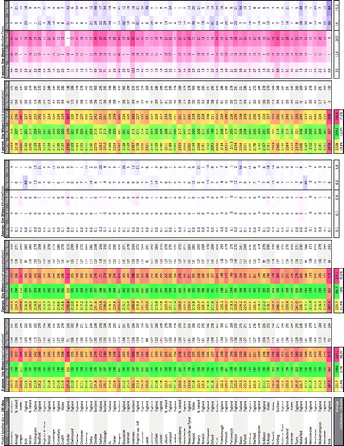
Interpretations of Figure 6 are manifold so only the most important will be highlighted here. First, it is necessary to state using the 3-p sine waves and the actual series of CRC values produced exactly the same estimated project durations for all cities and for all project start dates. This is not necessarily a surprise and the differences between these approaches may only be noticeable if the initial project duration is of the order of a few days, instead of a few months.

The duration estimates calculated using the 3-p sine waves indicate that the weather is likely to cause an extension to the original (weather-unaware) 186-d project duration by an average of 21.6%. However, this duration increase may be as large as 38.3%, or as small as 5.7%, depending on the start date. Therefore, if a project schedule was managed weather-wise (e.g. by carefully choosing the best project start date), average project durations could be reduced by 21.6–5.7% = 15.9%. Analogously, time proportional costs, like indirect and overhead costs, could also be reduced.

With the 2-p sine wave approximations, it can be seen that deviations in predicted project durations are almost always below 1 d (see the first three columns of the 2-p Sine Waves Absolute Errors). Identifying the optimum and worst project start days with regard to minimizing and maximizing project duration also on average remain below 1 week (see last two columns of the 2-p Sine Waves Absolute Errors). This is a very good approximation considering the simplicity of the 2-p expression being used to model an entire year day-by-day. Moreover, these predicted errors are the greatest over the year, and for the remainder of the year, deviations are much smaller.

In contrast, the 1-p sine wave curves produce significantly poorer approximations. This being said, average project duration errors remain below 3 d on average (see first columns of the 1-p Sine Waves Absolute Errors) which is in reality small and an upper bound. Projects longer than 6 months and/or those without non-working days will generally have less error. The shortest and longest project duration estimates, as well as their associated start dates err on average by less than 2 and 3 weeks, respectively (see the second and third columns of the 1-p Sine Waves Absolute Errors). In practice, these would not be considered bad estimates, especially as they come from such simple expressions with just one parameter. Moreover, similarly to the 2-p sine wave estimates, the errors quoted represent the largest possible errors and with longer projects or different project start dates, they are significantly reduced.

Discussion

The case study above shows how the sine waves proposed can be used with a straightforward approach to calculate individual activity and total project durations. Clearly, the possibility of calculating how long each activity will last depending on the start date and the location opens the door for further operational research applications. For example, it would be possible to analyse (a) how best to reduce project durations and costs when multiple projects have to be executed and their order can be modified; (b) how best to arrange non-critical activities to minimise durations and/or costs; and (c) how to select the best project location if that was a feasible option.

The proposed sine waves can also be applied with a stochastic approach instead of the discrete approach used in the case study here. In this case, each CRC daily value would be either 0 (workable day) or 1 (non-workable day), where the probability of the value being 0 or 1 would depend on the CRC calculated by the sine wave expression for each day. The CRC data series represent proportions of workable days from the past, but they can also be understood as ‘probabilities’ of a day being workable. This means that Monte Carlo simulations can be very easily implemented and used to calculate, through multiple iterations, a wide range of (probabilistic) project durations. This application, despite very interesting, goes beyond the aim of this paper, but, for the sake of promoting further research, a programmable spreadsheet has been included as Supplemental Online material which performs the Monte Carlo simulations described above.

Furthermore, the sine waves can also be employed in weather-aware schedules for calculating corresponding weather-unaware activity durations. This kind of forensic analysis would be of interest when dealing with weather-related claims. In this case, the actual activity durations (from the as-built schedule) have necessarily already been affected by the weather. Therefore, calculating the CRC values for each activity and adding them up from the actual activity start date until its finish date are all that is needed. Later, if an extended analysis is required, it would be possible to submit the calculated (weather-unaware) activity durations to Monte Carlo simulations. These simulations would provide the probabilistic project durations curve, from which it would be possible to determine the percentile to which the actual (as-built) schedule duration corresponded. This percentile would indicate whether some form of time and/or cost compensation would be appropriate, helping to mediate negotiations between contractors and clients. Again, despite giving more details about this application exceeds the aim of this paper, another programmable spreadsheet that performs ‘forensic’ weather scheduling analyses has been appended as Supplemental Online material.

Finally, although the sine wave method proposed may prove useful in many applications, it should be pointed out that it does have some limitations, even disadvantages. Regarding disadvantages, any project manager who is aware of the Parkinson’s law (project work expands to fill all the available time) will know that allowing for increased activity durations (due to weather or anything else) might lead to lower productivity levels. This productivity decrease might be caused by resources being more relaxed (on believing that they have more time than needed) or even by intentionally delaying the actual start dates due to the Student’s syndrome (delay to start working on a task until it becomes really urgent). A nice case explaining how pervasive these two phenomena can be for project progress can be found in Vanhoucke (2012, p. 188–189).

Then, the method proposed here anticipates longer activity durations, but that does not mean the resources will have extra time to work on them. They will have exactly the original planned time (because they will not be able to work during some days due to adverse weather conditions). It is the project manager’s responsibility to raise awareness on this issue and handle the resources as effectively as possible. Otherwise, further delays will occur.

However, concerning the proposed method limitations, the curves require data from as many weather stations as possible for improved accuracy and to make up for data sets that are not sufficient quality. This is not a problem in a country like the UK where weather stations are widespread and the data available spans many years. However, it could be an issue in other countries where there are significantly fewer and/or newer stations.

Moreover, the sine waves correspond to weather and thus workability at ground level (measurements taken at a height of 10 m). This means that for tall structures and/or for projects executed at sea, the curves may not be representative at all. Similarly, for projects located in very unusual and/or isolated regions where the climate is significantly different from nearby areas, the proposed sine wave curves may prove unrepresentative too.

However, there are many applications where the proposed sine waves will be more than sufficient, particularly as they are based on extremely simple mathematical expressions and allow for highly customisable combinations of weather variables.

A last cautionary note must be given before proceeding to the Conclusions section. On developing the case study, only deterministic scheduling analyses have been implemented. It is well known that, due to the Merge event bias¹ being neglected, deterministic schedules tend to underestimate the project duration (Ballesteros-Pérez 2017). Stochastic analysis has been intentionally not considered here for the sake of comparing homogeneous scheduling results (an original single weather-unaware deterministic schedule versus the remaining weather-aware, but also deterministic, schedules). This has allowed us to gauge the relative duration increases that are to be expected when introducing the weather factor. But also avoiding other sources of potential bias like activity duration variability present in the original weather-unaware schedule. Finally, the case study developed consisted of a schedule with very few activities in parallel. This made the potential project duration underestimations a very minor cause of concern in this occasion. For future scheduling analyses, though, Monte Carlo simulations like the ones that can be performed in the spreadsheets included as Supplemental Online material, are recommended.

Conclusions

Construction projects involve multiple weather-sensitive activities that frequently cause significant project delays and economic losses for both contractors and project owners. A significant proportion of infrastructure-related activities (from construction to operation and maintenance) are highly weather-sensitive, as they are mostly performed outdoors. This weather sensitivity, however, varies according to the nature of each activity, as well as the location and season in which they are carried out. Furthermore, different activities are susceptible to different combinations of weather variables (e.g. temperature, rain and wind) and their intensities.

Quantitative research on the influence of weather on construction productivity is scarce, predominantly less than 10 years old, and focuses mostly on building construction. Therefore, the main aim of this paper was to propose a method that allows construction industry professionals to plan in the medium- and long-term (beyond 2 weeks) considering the seasonal variation of weather. The method proposed is not limited to a small number of weather variables, nor to small geographical areas, and allows for many types of project activities to be considered.

The major contribution of this research is the development of a series of sine wave expressions that model quite closely the average probability of a day being workable for a particular type of activity. The curves also allow a planner to anticipate how much longer a project activity will take to complete as a consequence of the weather. The proposed calculations can cover all days of the year, and by selecting appropriate combinations of weather variables, can be defined for different types of activities and projects. Moreover, the expressions can be implemented with either one, two or three parameters depending on the degree of accuracy required.

Most construction projects comprise hundreds (sometimes thousands) of weather-sensitive activities which interact through a precedence network (e.g. certain activities must be completed before others can start). Ascertaining the weather sensitivity of a whole project requires combining the weather’s impact on multiple activities and determining the ensuing effect on the overall project duration.

In this paper, six frequent and standard construction activities were defined and the weather variable combinations and intensities commonly accepted as preventing them from being executed were justified. Using data from 102 weather stations and applying the relevant constraints, sine wave expressions corresponding to the six types of construction activities were calculated.

A case study involving the construction of a reinforced concrete building was used to demonstrate how these sine waves can be applied in the prediction of project durations. The findings from the case study indicate that UK weather can extend building project durations, on average by 21%. Furthermore, planning to minimise potential weather-related delays can lead to average project duration reductions of 16%, with associated indirect and overhead cost reductions.

Finally, some limitations and further applications of the proposed sine wave expressions were discussed. Among these applications, the use of the sine waves for stochastic weather-aware scheduling and in dealing objectively with weather-related claims is the most relevant. However, it is likely that many other applications of this research will be found in the future. Finally, to facilitate use of the model, the majority of the data analysis, results (contour maps of the UK), and programmable spreadsheets for performing both deterministic and stochastic project scheduling calculations have all been included as Supplemental Online Material.

Acknowledgement

Weather data were supplied by the UK Met Office (MIDAS data set).

Disclosure statement

No potential conflict of interest was reported by the authors.

Note

Additional information

Funding

This work was supported by the CIOB Bowen Jenkins Legacy Research Fund under [Grant number BLJ2016/BJL.01]; and NERC with the Environmental Risks to Infrastructure Innovation Programme under [Grant number NE/R008876/1].

Notes

1 Actually, the merge event bias is nothing but a special case of Jensen’s inequality. This, as the maximum of the average durations of multiple activities which are performed in parallel is always equal to or lower than the average duration of the maximum of such activity durations.

References

- Alaghbari, W., et al., 2007. The significant factors causing delay of building construction projects in Malaysia. Engineering, construction and architectural management, 14, 192–206.
- Alarcón, L.F., et al., 2005. Assessing the impacts of implementing lean construction. In: Proceedings for the 13th International Group for Lean Construction Annual Conference, 25–27 July 2006, Santiago. Sydney, Australia: International Group on Lean Construction, 387–393.
- AlSehaimi, A. and Koskela, L. 2008. What can be learned from studies on delay in construction? In: Proceedings for the 16th Annual Conference of the International Group for Lean Construction, 16–18 July 2008. Manchester, UK: International Group on Lean Construction, 95–106.
- American Concrete Institute. 1985. Manual of concrete practice, Part 1. Detroit, MI: American Concrete Institute.
- Apipattanavis, S., et al., 2010. Integrated framework for quantifying and predicting weather-related highway construction delays. Journal of construction engineering and management, 136, 1160–1168.
- Assaf, S.A. and Al-Hejji, S., 2006. Causes of delay in large construction projects. International journal of project management, 24, 349–357.
- Ballesteros-Pérez, P., 2017. M-PERT: a manual project duration estimation technique for teaching scheduling basics. Journal of construction engineering and management, 143 (9), 4017063.
- Ballesteros-Pérez, P., et al., 2015. Climate and construction delays: case study in Chile. Engineering, construction and architectural management, 22, 596–621.
- Ballesteros-Pérez, P., et al., 2017a. Dealing with weather-related claims in construction contracts: a new approach. In: ISEC 2017 – 9th International Structural Engineering and Construction Conference: Resilient Structures and Sustainable Construction, 24–29 July 2017. Valencia, Spain: ISEC Press.
- Ballesteros-Pérez, P., et al., 2017b. Weather-wise: a weather-aware planning tool for improving construction productivity and dealing with claims. Automation in construction, 84, 81–95.
- Chinowsky, P., et al., 2013. Climate change adaptation advantage for African road infrastructure. Climatic change, 117, 345–361.
- David, M., et al., 2010. A method to generate typical meteorological years from raw hourly climatic databases. Building and environment, 45, 1722–1732.
- Duffy, G., et al., 2012. Advanced linear scheduling program with varying production rates for pipeline construction projects. Automation in construction, 27, 99–110.
- Dytczak, M., et al., 2013. Weather influence-aware robust construction project structure. Procedia engineering, 57, 244–253.
- El-Rayes, K. and Moselhi, O., 2001. Impact of rainfall on the productivity of highway construction. Journal of construction engineering and management, 127, 125–131.
- Finke, M.R., 1990. Weather-related delays on government contracts. In: AACE International Transactions of the Annual Meetings, Association for the Advancement of Cost Engineering International (AACEI), 24–27 June 1990, Boston, MA. Morgantown, WV: AACE.
- Głuszak, M. and Les¨niak, A., 2015. Construction delays in clients opinion – multivariate statistical analysis. Procedia engineering, 123, 182–189.
- González, P., et al., 2014. Analysis of causes of delay and time performance in construction projects. Journal of construction engineering and management, 140, 4013027.
- Gündüz, M., Nielsen, Y., and Özdemir, M., 2013. Quantification of delay factors using the relative importance index method for construction projects in Turkey. Journal of management in engineering, 29, 133–139.
- Hamzah, N., et al., 2011. Cause of construction delay – theoretical framework. Procedia engineering, 20, 490–495.
- Irizarry, J., Simonsen, K.L., and Abraham, D.M., 2005. Effect of safety and environmental variables on task durations in steel erection. Journal of construction engineering and management, 131, 1310–1319.
- Jang, M.H., et al., 2008. Method of using weather information for support to manage building construction projects. In: M. Ettouney, ed. AEI 2008: building integration solutions. Reston, VA: ASCE, 1–10. doi:10.1061/41002(328)38
- Jung, M., et al., 2016. Weather-delay simulation model based on vertical weather profile for high-rise building construction. Journal of construction engineering and management, 142, 4016007. doi:10.1061/(ASCE)CO.1943-7862.0001109
- Kim, S.H. and Augenbroe, G., 2012. Using the national digital forecast database for model-based building controls. Automation in construction, 27, 170–182.
- Kumaraswamy, M.M., 1997. Conflicts, claims and disputes in construction. Engineering, construction and architectural management, 4, 95–111.
- Li, X., et al., 2016. Evaluating the impacts of high-temperature outdoor working environments on construction labor productivity in China: a case study of rebar workers. Building and environment, 95, 42–52.
- Mahamid, I., Bruland, A., and Dmaidi, N., 2012. Causes of delay in road construction projects. Journal of management in engineering, 28, 300–310.
- Marzouk, M. and Hamdy, A., 2013. Quantifying weather impact on formwork shuttering and removal operation using system dynamics. KSCE journal of civil engineering, 17, 620–626.
- Matheron, G., 1969. Part 1 of Cahiers du Centre de morphologie mathématique de Fontainebleau. Le krigeage universel. École nationale supérieure des mines de Paris.
- Mentis, M., 2015. Managing project risks and uncertainties. Forest ecosystems 2, 1–14. doi:10.1186/s40663-014-0026-z
- Mezher, T.M. and Tawil, W., 1998. Causes of delays in the construction industry in Lebanon. Engineering, construction and architectural management, 5, 252–260.
- Moselhi, O. and El-Rayes, K., 2002. Analyzing weather-related construction claims. Cost engineering, 44, 12–19.
- National Cooperative Highway Research Program (NCHRP). 1978. Effect of weather on highway construction. NCHRP Synthesis 47, Transportation Research Board, FL, USA.
- Nguyen, L.D., et al., 2010. Analysis of adverse weather for excusable delays. Journal of construction engineering and management, 136, 1258–1267.
- Orangi, A., Palaneeswaran, E., and Wilson, J., 2011. Exploring delays in Victoria-based Australian pipeline projects. Procedia engineering, 14, 874–881.
- Rogalska, M., et al., 2006. Methods of estimation of building processes duration including weather risk factors (in Polish). Building review, 1, 37–42.
- Ruqaishi, M. and Bashir, H.A., 2015. Causes of delay in construction projects in the oil and gas industry in the gulf cooperation council countries: a case study. Journal of management in engineering, 31, 5014017. doi:10.1061/(ASCE)ME.1943-5479.0000248
- Sato, K., et al., 2017. Improved forecasts of winter weather extremes over midlatitudes with extra Arctic observations. Journal of geophysical research: oceans, 122, 775–787.
- Shahin, A., AbouRizk, S.M., and Mohamed, Y., 2011. Modeling weather-sensitive construction activity using simulation. Journal of construction engineering and management, 137, 238–246.
- Shahin, A., et al., 2014. Simulation modeling of weather-sensitive tunnelling construction activities subject to cold weather. Canadian journal of civil engineering, 41, 48–55.
- Shan, Y. and Goodrum, P.M., 2014. Integration of building information modeling and critical path method schedules to simulate the impact of temperature and humidity at the project level. Buildings, 4, 295–319.
- Tanijiri, H., et al., 1997. Development of automated weather-unaffected building construction system. Automation in construction, 6, 215–227.
- Thomas, H.R., Riley, D.R., and Sanvido, V.E., 1999. Loss of labor productivity due to delivery methods and weather. Journal of construction engineering and management, 125, 39–46.
- Thorpe, D. and Karan, E.P. 2008. Method for calculating schedule delay considering weather conditions. In: Proceedings 24th Annual ARCOM Conference, 13 September 2008, Cardiff, UK. pp. 809–818.
- Tian, W. and De Wilde, P. 2011. Uncertainty and sensitivity analysis of building performance using probabilistic climate projections: a UK case study. Automation in construction, 20, 1096–1109.
- Trauner, T.J., et al., 2009. Construction delays, understanding them clearly, analyzing them correctly. Burlington, MA: Elsevier.
- UK Met Office. 2018. Met Office Integrated Data Archive System (MIDAS) Land and Marine Surface Stations Data (1853-current). Available from: http://catalogue.ceda.ac.uk/uuid/220a65615218d5c9cc9e4785a3234bd0 [Accessed 8 March 2018].
- Vanhoucke, M., 2012. Project management with dynamic scheduling: baseline scheduling, risk analysis and project control. Berlin and Heidelberg: Springer.
- Vose, R.S. and Menne, M.J., 2004. A method to determine station density requirements for climate observing networks. Journal of climate, 17, 2961–2971. doi:10.1175/1520-0442(2004)017<2961:AMTDSD>2.0.CO;2
- White, C.J., et al., 2017. Potential applications of subseasonal-to-seasonal (S2S) predictions. Meteorological applications, 24, 315–325.
- Yogeswaran, K., Kumaraswamy, M.M., and Miller, D.R.A., 1998. Claims for extensions of time in civil engineering projects. Construction management and economics, 16, 283–293.