Modeling of In-Line Tube Banks Inside Advanced Gas-Cooled Reactor Boilers

Abstract

The objective of this research is the prediction of forced convection across confined in-line tube banks found in Advanced Gas-Cooled Reactor (AGR) boiler systems. The focus of this work is periodic flow about a 2 × 2 array. A number of Reynolds-Averaged Navier–Stokes (RANS) turbulence modeling closures have been applied to the challenging case of 1.6 pitch-to-diameter spacing at which flow undergoes transition from straight to diagonal. In contrast to Large Eddy Simulation (LES) predictions, those of RANS models fail to predict transition to diagonal flow. As LES computations are not anticipated to become routine enough for the purpose of flow diagnostics in industrial contexts for many years, further refinement to the RANS methodology in the form of an analytical wall function is one of the main objectives. Its eventual inclusion is not only expected to improve the representation of turbulent boundary layer behavior, but also has scope to account for augmented surface roughness effects experienced by AGR technologies nearing their end-of-life. This work is ultimately in aid of EDF Energy’s policy of AGR lifetime extensions, to allow the UK Government sufficient time to formulate a credible Nuclear New Build scheme to secure our energy requirements in the coming decades. It was found that all but dynamic LES adequately reproduces flow behavior across all criteria considered, and that standard wall functions left much to be desired in the case of flow and thermal predictions, while introducing the analytical wall function generates improvements for flow and heat transfer predictions that are not universally shared between high-Re models utilized.

Introduction

Tubular cross-flow heat exchangers see extensive use in power generation or heavy process industries, such as civil power generation, chemical production and synthesis facilities, desalination plants, oil refineries, and many others. Heat exchangers which make use of tube bank geometries have even been suggested in the design of the precooling system to be used by Reaction Engines Ltd.’s ground-to-space vehicle SABRE engine [1]. Despite their apparent ubiquity, the flows about clusters of tubes, particularly those subject to being densely packed in the presence of confining walls, are poorly understood, even before the case is made to account for the effects of turbulence on the momentum and thermal domains. The primary focus of this work is to inform EDF Energy of the flow environment present within their serpentine boiler tube systems deployed on the later designs of Advanced Gas-Cooled Reactors (AGRs), having some provision to account for the effects of ageing on the tubes themselves. Ageing effects have become a source of concern for the operation of the UK’s civil nuclear fleet, as fatigue damage due to flow unsteadiness has set in, in addition to the radiolytic dissociation of the carbon dioxide coolant into oxygen and carbon particulates, the latter of which leads to augmented roughness and impairment of heat transfers through working surfaces. EDF Energy’s current policy is to develop means of ensuring that existing energy generation capacity can continue to be operated safely beyond the original anticipated closure dates through the Plant Lifetime Extension scheme, as has been done with Dungeness B in late 2015 [2], to allow the UK Government sufficient time to formulate a credible Nuclear New Build strategy to secure our low-carbon energy supply in the coming decades. Reactor longevity is largely determined by either the long-term performance of the irradiated graphite core, or the boiler tube platens which are the subject of this work. Accessibility to the system for repairs is severely impractical due to the reactor pressure vessel and boilers being surrounded by walls of pre-stressed concrete four meters in thickness, though attempts at cleaning have been made on affected working heat transfer surfaces by injecting oxygen jets into the secondary coolant loop. However, the position of these jets about the periphery, which themselves are only targeted at the secondary superheaters of the outboard platens, has led to non-uniform cleaning circumferentially. In short, the system is becoming increasingly difficult to operate as a result of ageing introducing non-uniform off-design conditions, leading to a forced non-uniform response by operators in attempt to alleviate their detrimental effects, giving a highly complex thermal hydraulics environment even before the presence of turbulent flow is considered. To prevent feedwater escaping through damaged tubes into the primary coolant circuit and coming into contact with the irradiated high-temperature graphite, some of the tubes have been deliberately blanked off, which adds inconsistent heat extraction through the remaining tubes to the problem. The turbines expect a steady supply of steam at 525 kg s⁻¹ at 814.15 K [3], and so in the face of blanked tubes, the remaining feedwater supply through the platens must be altered to maintain the thermal equilibrium necessary to generate a sufficient quantity of steam at the correct temperature for which the turbines are rated to prevent further thermodynamic efficiency losses. Ultimately, layers of non-uniform difficulties are present, where the only viable countermeasures to operators were non-uniform, in a highly complex flow environment subject to turbulence and heat transfers in the presence of walls with variable roughness. There exists a significant dearth of recent experimental work addressing tube banks in general, especially involving arrays of in-line tubes, and the studies which are publicly available are more concerned with the vorticity shedding characteristics of the system as opposed to the static pressure or heat transfer profiles of individual tubes. Possible reasons for this state of affairs include the sheer complexity of fully instrumenting an array of greater than around 20 tubes with pressure transducers, heat sources/sinks and thermocouples versus the comparatively simple case of inducing a flow over tube bank geometry and injecting a dye stream to track the evolution of flow using high-speed cameras. Of the limited experiments which have been performed, the focus has been overwhelmingly in favor of staggered tube banks instead of the in-line variety being examined here. The fundamental arrangements for in-line and staggered arrays of tubes are shown in Figure 1, where any deviation in configuration from these is performed by modifying the transverse and longitudinal pitches of the two primitive arrays shown, e.g. rotated square arrays, normal and parallel triangular arrays, or modifications of the individual tube surface geometries, such as the addition of exterior fins.

At low velocities, where the flow through each of the arrays lies firmly in the laminar regime, it can be seen that left-to-right flow within an in-line bank as depicted is prone to sequential accelerations and decelerations as the transverse spacing between tubes narrows and widens, while in the staggered array, the flow can navigate about each individual tube without undergoing significant flow area changes, giving a steadier flow overall. The staggered array tends to achieve greater heat transfer as a result of this, as for a given left-to-right flow Reynolds number, longitudinal and transverse pitch-to-diameter ratios, there is more longitudinal space between tubes in the same row when compared with an in-line case, such that their wakes have less tendency to impinge on succeeding tube surfaces. As a result, wakes are less likely to become trapped between tubes in the same column, blocking warmer flow from making direct thermal contact with working heat transfer surfaces. This comes with the penalty of slightly increased manufacturing and implementation complexity on a given exchanger, usually by suspending tube platens slightly lower or higher in an alternating pattern, necessitating either greater numbers or interchanging locations of welds. As the velocity enters the subcritical flow regime, typified by a circumferential laminar-to-turbulent transition in the boundary layers about the tube surfaces, in the in-line case, the flow opts to follow a diagonalized path [4] (in the absence of confining walls), rather than expend excess energy being continuously accelerated and decelerated following a straight-through trajectory. In this flow regime, the resultant flow depends less on the bulk Reynolds number, and more upon two geometric parameters: the longitudinal and transverse pitch-to-diameter ratios [5]. This is a result of the flow being governed predominantly by proximity and wake interferences and other blockage effects rather than its energy content. P_L and P_T denote the longitudinal and transverse pitches respectively, while the relevant length scale for the Reynolds number in this case is the tube diameter, D. Tube bank geometries are also broadly categorized by whether or not they are compact, which is the product of their longitudinal and transverse pitch-to-diameter ratios as follows: (1) $$\text{For given}\frac{P_L}{D}\&\frac{P_T}{D},\mathrm{ }\mathrm{if}:\mathrm{ }\left\{\begin{array}{c}\frac{P_L{P}_T}{D^2}<{1.25}^2 \mathrm{Array} \mathrm{is} \mathrm{deemed} \mathrm{compact}\\ \frac{P_L{P}_T}{D^2}>4\mathrm{ }\mathrm{Array} \mathrm{is} \mathrm{widely}-\mathrm{spaced}\hfill \end{array}\mathrm{ }\right.$$(1)

Tube banks lend themselves readily to heat transfer processes between two media, typically either a matrix of tubes carrying cooler fluid through a hotter solid, or as is the case in a cross-flow exchanger, where a warm fluid is driven transversely through the array while a cooler working fluid is pumped normally through the tubes. Such configurations encourage high levels of heat transfer with relative ease of manufacture, and consequently they see widespread use in mechanical and chemical engineering applications. Though flow through a compact in-line tube bank tends toward diagonalized flow in an infinite array, engineering flows are bounded by walls, which typically have the effect of forcing flow to traverse the multi-tube array (the preferred term for tube bank geometries subject to confinement) in a straight-through fashion, at least on average. It is worth noting that flows of any practical value flowing about these geometries are notably unsteady, where as many as five distinct flow patterns may arise in the subcritical regime dependent on longitudinal and transverse spacing (though neatly delineating the spacing at which some flow-fields end and others begin is challenging) [6].

Three of the five patterns which have been observed are illustrated in Figure 2 [6]. It has been reproduced here due to the poor image quality of the original source. Pattern A indicates that flow behind each individual cylinder has just enough space to form von Kármán-Bénard vortices, where each vortex impinges upon immediately succeeding tubes, leading to flow behind each tube being 180° out of phase with the one immediately preceding it. In the case of Pattern B, where the array is more packed longitudinally, this out-of-phase phenomenon persists, however, what is referred to as “jet-swinging” flow takes place, where the wakes behind tubes are entirely deflected diagonally as the flow seeks greater space to flow through. Pattern C merely displays a case where the tubes are so packed that the wakes that form become trapped behind the cylinders and the next succeeding row, meaning the bulk of the flow is straight-through in the undisturbed flow lanes. Pattern D entails biased-bistable flow between rows of tubes, and demonstrates the “lock-in” flow feature [7] characteristic of rows with tubes with narrow transverse gaps but large longitudinal pitch, where the wakes behind tubes which neighbor one another in the vertical direction are not symmetric in time, i.e. one wake grows in time whilst the other diminishes, giving a significant angular deviation for flow exist in time. Additionally, this wake development and reduction varies in time (not necessarily with a clear periodicity), meaning that flow which is deflected angularly in one direction initially changes its trajectory to reflect which wake in the pair is growing or suppressed. Such behavior is case-specific to the geometric configuration under scrutiny; however they all share time-dependent flow deflections in common [8]. Finally, Pattern E entails the simple case whereby all of the cylinders in the array are sufficiently far apart in both longitudinal and transverse pitch that the flows around each are essentially identical to tubes in complete isolation. The dashed line on the diagram denotes the additional numerical studies performed that suggested delineating between Patterns A, B, and C is somewhat problematic (and misleading), especially in the case of compact banks, as which pattern a flow will fall into depends on other factors such as freestream turbulence intensities and surface roughness levels, in addition to the Reynolds number [9]. The geometry of interest to EDF Energy also features a further complication in that the longitudinal pitch of the tubes within a serpentine tube boiler platen alternates over its length, namely, that tubes are bunched together in pairs, with a larger longitudinal gap behind these and the following pair of tubes, however, the transverse pitch is maintained constantly throughout. Correspondingly, one would expect the flow pattern through such a configuration to be an amalgam of Patterns A and B, where wakes about the first pair of tubes may initially be trapped, and developing unsteadiness generates more apparent jet-swinging in the remainder of the array.

Methodology

As an initial test case, this work considers turbulent flow about a square in-line tube bank consisting of circular tubes, with a constant pitch-to-diameter ratio of 1.6, which is modeled using periodic boundary conditions to reduce the computational domain. Simulating such geometry is applicable to conditions found deep within a tube bank that are free from significant entry and exit effects, conditions which are deemed valid beyond the first four, and before the final four, rows of tubes [10]. Since periodicity is employed, and the flow essentially encounters an indefinite array, either a mass flow rate or a pressure gradient must be prescribed to force the flow to reach a fully-developed state, as opposed to its momentum slowly decaying to zero in time. Similarly, a thermal balance must be struck via cell-weighted volumetric heating to match the thermal energy being extracted through the tube boundaries to prevent the temperature tending to absolute zero. In the case of momentum, a self-correcting mean pressure gradient is supplied, in which a target Reynolds number is prescribed, and a linear under-relaxation method is used to iterate towards it in time. Thermal conditions are handled using the approach of Acharya et al. [11], where the temperature field in the domain is decomposed into the sum of linear and periodic parts, such that the linear portion reflects the bulk temperature gradient over the finite domain in the dominant flow direction, while the periodic portion is continuously fed back between the periodic inlet and outlet boundary conditions and vice versa. When a periodic boundary is encountered, Code_Saturne generates fictitious ‘halo’ or ‘ghost’ cells that are mirror images of cells adjacent to periodic boundaries, interpolates between these outermost cells and their ‘ghosts’ to determine the value of temperature at the outlet boundaries, then feeds these values back to the corresponding inlet boundaries. In this way, the flow bulk momentum and temperature variations in the domain are captured through the linear term, while the periodic term ensures no information is lost in time as the flow enters or leaves. By exactly matching source terms to these linear changes, momentum and thermal balances can be reached in time, beyond which no further variations in bulk temperature or momentum are seen. The pressure and temperature source terms, denoted by β and γ, respectively are defined as follows from Eqs. (2)–(6). Q is the linear under-relaxation coefficient, where a value of 3.125 × 10⁻⁴ was found to give satisfactory convergence to the target Reynolds number, Re_ref = 4.1 × 10⁴_. (2) $$P\left(x,y,z,t\right)=\mathrm{ }-\beta x+P_{\mathit{Perio}}\left(x,y,z,t\right)$$(2) (3) $$\mathrm{\Theta }\left(x,y,z,t\right)=\mathrm{ }\mp \gamma x+{\mathrm{\Theta }}_{\mathit{Perio}}\left(x,y,z,t\right)$$(3) (4) $$\beta =\frac{\partial P}{\partial x}$$(4) (5) $${\mathrm{ }\beta }^{\left(n+1\right)}=\mathrm{ }{\beta }^{\left(n\right)}+Q\left(R{e}_{\mathit{ref}}-\mathit{Re}\right)$$(5) (6) $$\gamma =\frac{\partial {\mathrm{\Theta }}_{\mathit{bulk}}}{\partial x}\equiv \frac{q_{\mathit{wall}}}{\rho U_{\mathit{bulk}}{c}_{p}D}\mathrm{ }$$(6)

Provided the momentum and thermal balances are maintained throughout the calculation, a flow-field with constant velocity and temperature can be initialized, which then evolves into a fully-developed flow case at the target Reynolds number. However, while the solution does eventually mature into repeating conditions where a clear periodicity is established, temporal and spatial averaging must be performed to output flow parameters of interest. Thermal isoflux boundaries are applied over all tube surfaces considered. Turbulent conditions inevitably result at the Reynolds number desired, necessitating the use of a variety of turbulence modeling closures to obtain solutions. This work makes extensive use of Code_Saturne version 4.0.3. [12], a computational fluid dynamics collocated finite-volume solver developed by EDF R&D, to simulate the flows about such geometries. Code_Saturne also carries with it the advantage of being freely available and open-source, allowing for users to tailor the code using subroutines to meet their specific requirements. Several versions of it are also widely installed on UK supercomputing facilities, such as the N8 HPC and ARCHER clusters. A wide range of turbulence models have already been implemented in the code, where examples of Reynolds-Averaged Navier–Stokes (RANS) models range from the progenitor k-ε [13] models using high-Re approaches regarding near-wall regions, to elliptically blended Reynolds stress transport models [14] which need full resolution of the boundary layer, requiring fine grids in boundary regions. In addition, a number of Large Eddy Simulation (LES) sub-grid scale models are available, including both static and dynamic Smagorinsky models [15, 16]. For the RANS computations, meshes of 528,000 cells and 1,456,000 cells were utilized for models reliant upon standard logarithmic law wall functions for high-Re turbulence models and full boundary layer resolution for low-Re turbulence models, respectively, while the dynamic LES approach adopted here utilized a mesh of 5.2 M cells. All meshes employed by this study are shown under Figure 3, within dedicated subfigures. The individual cases run are listed in Table 1 by turbulence models used, their corresponding wall treatments, and upon which grids under Figure 3 along with their cell counts. All cases considered herein are fully three-dimensional, and have employed block-structured hexahedral meshing to maintain greater control of the size and density of cells in the domain. The results of an earlier mesh independency study using the k-ω Shear Stress Transport (SST) model are shown in Figure 4, where the circumferential resolution is 240 cells, yielding an angular resolution of 1.5° (as opposed to the 200 cells used in a previous study, which was found to be sufficient [4]), and the spanwise resolution is varied between 4, 8, 16, and 20 per diameter of tube length, where the tube is two diameters long. It can be seen that mesh independency is reached at a spanwise resolution of 16 cells per diameter, but remaining results adopted 20 cells per diameter as a numerical precaution, since the change in computational cost was not significant. The adequacy of the source term approach for approaching the target Reynolds number is displayed under Figure 5, where it can be seen that all calculations converge to within ±0.2 of the desired 41,000 over the course of the simulations run across all meshes and varieties of turbulence models employed. With regards to time-averaging, Figure 6 shows the periodic signals for lift and drag coefficient obtained by the R_ij-ε Speziale-Sarkar-Gatski (SSG) model using the high-Re grid under Figure 3. The lift coefficient signal was then decomposed into its dominant frequencies using a Fast Fourier Transform, which was then re-expressed in terms of Strouhal number, as shown under Figure 7. A strong Strouhal number dominance is seen at 0.162, which translates to a frequency of oscillation of 2.458 Hz, safely within the time-averaging window of 3,500 s of simulation time. Fluid property variations with temperature have not yet been appraised. The experimental data of Aiba et al. [17] document a square in-line bank with spacing matching that of the case being simulated using the periodicity approach, and so provides a convenient point of comparison for the generated results. In the experimental setup, the surface pressure and heat transfer levels were reported at 10° intervals, using pressure tapping holes of 0.5mm diameter and a tungsten hot-wire anemometer of 0.005 mm in thickness with an effective length of 1 mm [17], where the measured cylinder surface was electrically heated using a helically wound stainless steel ribbon 0.05 mm in thickness, and the thermal results reported were obtained under the conditions of constant heat flux, as also prescribed in the simulation. Though the experimental working fluid was air, which is known to be insensitive to Prandtl number changes over a large temperature range (similarly to carbon dioxide, used for the simulation), the decision was taken to measure the pressure and heat transfer distributions independently rather than in tandem, i.e. no heating was supplied when obtaining the static pressure results [17]. This is a standard approach used by experimentalists, as it eliminates the possibility of any changes to the flow’s near-wall behavior due to thermal energy supplied by the apparatus itself, as opposed to that which it would already possess under ambient conditions. To prevent heat leakage, the inside of the measured cylinder was insulated using polyurethane foam, to minimize heat loss through mechanisms other than the forced convection case of interest [17]. The full-scale appraisal of EDF Energy’s geometry will be non-periodic, and so will not require the momentum and thermal balances in the simulation work outlined above, its solution can simply be initialized with the representative operating conditions for the secondary superheater outlined by Nonbøl [3] at the inlet, and the resulting flow can be examined directly.

Table 1. All configurations of cases run in this study, delineated by turbulence models used, wall treatment strategies, and the corresponding grids utilized as listed under Figure 3.

Turbulence model	Wall treatment(s)	Grid (Corresponding Figure, cell count)
k-ε LP	Standard wall function and analytical wall function	High-Re Grid (Figure 3a, cell count: 528,000)
k-ω SST	Resolved boundary layer to y* ≤ 1	Low-Re Grid (Figure 3b, cell count: 1,456,000)
ϕ-f	Resolved boundary layer to y* ≤ 1	Low-Re Grid (Figure 3b cell count: 1,456,000)
Rij-ε SSG	Standard wall function and analytical wall function	High-Re Grid (Figure 3a, cell count: 528,000)
Rij-ε EB-RSM	Resolved boundary layer to y* ≤ 1	Low-Re Grid (Figure 3b, cell count: 1,456,000)
LES (Dynamic)	Resolved boundary layer to Δy* ≤ 1 (including Δx^+ < 20 and Δz^+< 40 globally)	LES Grid (Figure 3c, cell count: ∼5,200,000)

A dilemma arises in that given the computing resources available, a wall-resolved LES of the full geometry is simply untenable; the same is likely true even of a low-Re Unsteady Reynolds-Averaged Navier–Stokes (URANS) strategy also. Consequently, a high-Re methodology of appraising the flow is essentially the only realistic way forward; however, these results indicate evident weaknesses when following such a route to closure. For that reason, the decision was made that a fundamental change to the handling of near-wall regions in high-Re turbulence models was warranted, from the point of view of acquiring realistic results in a computationally and time efficient manner. The implementation of the Analytical Wall Function (AWF) of Suga et al. [18] stands a fair chance of improving the frictional and heat transfer predictions about the central tube, and carries with it the potential to account for the augmented surface roughness on ageing AGR systems for the full platen case. Additionally, it contains alternative formulations with regards to whether or not a boundary cell is within either the flow’s viscous sublayer or outside of it and prone to near-wall turbulence effects, meaning it behaves similarly to a scalable wall function and is more numerically robust, which standard log-law formulations cannot permit. It has been primarily pursued because of its unique ability to capture the effects of near-wall roughness in a manner consistent with the erosion of the viscous sublayer and limitation of near-wall convection, leading to recirculating pockets of flow between roughness elements. This forms a thermally insulating barrier between the working heat transfer surface and the warm bulk flow, which relates to the research questions posed by EDF Energy to determine heat transfer impairment and boiler system longevity, though said formulation and its associated results are not documented here. Furthermore, it does not constitute much by way of additional computational requirements, and can allow for flow separations and reattachments to be captured more appropriately through the solution of simplified analytical transport equations for momentum and thermal transport processes. Admittedly, however, there exists some empiricism within the method, as even after the Navier–Stokes equations are simplified to their boundary-layer form, the resultant system has not yet been solved in a purely analytical sense from first principles alone in a turbulent case, in addition to discretization errors being unavoidable. The assumptions made by the AWF are listed below:

1. Diffusion of momentum and thermal energy is dominant in the wall-normal direction

2. The pressure gradient is constant across a near-wall cell

3. The variation of turbulent viscosity is readily integrable (i.e. prescribed)

4. Convection of momentum and thermal energy normal and parallel to walls are constant in near-wall cells

Assumptions A and B are the laminar boundary layer approximations used to obtain the Blasius solution for attached boundary layers [19], while Assumptions C and D render the prospect of obtaining a solution under turbulent conditions tractable. The empiric aspects feature predominantly in Assumption C, where the prescribed variation is linear based on increasing normal distance above an assumed viscous sublayer height of 10.88 non-dimensional units, below which only molecular viscosity acts. The precise formulation for the entirety of the smooth-walled AWF model can be found in the Appendix.

Results and discussion

The exhaustive list of RANS turbulence model closures used consists of the k-ε Linear Production (LP) [20] and k-ω SST [21] two-equation models, the elliptic-relaxation φ-f model [22] (itself a numerical analog of the v²-f elliptically relaxed model proposed by Durbin [23]), the R_ij-ε SSG high Re second moment closure suggested by Speziale et al. [24], and the low-Re Elliptic-Blending Reynolds Stress Model (EB-RSM) put forward by Manceau and Hanjalić [25]. Owing to the geometry’s complexity, of the LES options available, only the dynamic formulation using a variable Smagorinsky constant has been employed, since arbitrarily assigning a single Smagorinsky constant to determine the sub-grid length scale casts doubt upon the solution’s dependability. Qualitative results include filled velocity and thermal contours of the time-averaged flow domain along the mid-span of the tubes. Quantitative results are mainly limited to non-dimensional flow quantities, which in the case of the tube bank outputs include the time and space-averaged static pressure coefficient, friction coefficient, and non-dimensional heat transfer in the form of the Nusselt number, where the non-dimensional quantities are defined in Eqs. (7)–(9). (7) $$\overline{C_P}=\overline{\frac{p-p_{\mathrm{\infty }}}{\frac{1}{2}\rho U_{\mathit{bulk}}^2}\mathrm{ }}$$(7) (8) $$\overline{C_f}=\mathrm{ }\overline{\mp \frac{{\tau }_{\mathit{wall}}}{\frac{1}{2}\rho U_{\mathit{bulk}}^2}}\mathrm{ }$$(8) (9) $$\overline{\mathit{Nu}}=\overline{\frac{q_{\mathit{wall}}D}{\lambda \mathrm{\Delta }\mathrm{\Theta }}}\equiv \overline{\frac{\mathit{hD}}{\lambda }}\mathrm{ }$$(9)

Indicative of the challenge posed by this flow case on the traditional RANS methodologies for simulating turbulence, there is a large disparity between the results obtained between the models which require the use of wall functions and those which resolve the boundary layer to within y* ≤ 1. Figures 8–10 show the results for time-averaged pressure coefficient about the central tube using all models and wall treatments considered herein, Figures 11–13 display the equivalent for friction coefficient, while Figures 14–16 show the corresponding Nusselt number distributions. As a general rule, the low-Re models suggest that the flow follows an alternating asymmetric pattern in time, that is, where flow undulates behind each tube and successive wakes are 180° out-of-phase, averaging to largely symmetric flow and heat transfer in time. This can be seen on Figures 8, 11, and 14, where all the results obtained other than by dynamic LES indicate an almost exact symmetry about the tube centerline at 180° (in the case of Figure 14, this can be inferred by the magnitudes of peaks and troughs being similar, due to the sign convention adopted in Eq. 8(8) $$\overline{C_f}=\mathrm{ }\overline{\mp \frac{{\tau }_{\mathit{wall}}}{\frac{1}{2}\rho U_{\mathit{bulk}}^2}}\mathrm{ }$$(8) ). However, the high-Re models using standard wall functions anticipate persistent asymmetry of flow, where there exists an angular deflection from the initial straight-through flow to a diagonalized trajectory which is maintained, albeit with some instability in the wake due to vorticity shedding. This yields a definitive angular deflection in the time-averages for all the standard URANS model cases, where clear peaks in static surface pressure and heat transfer can be seen favoring one side of the tube about the centerline over the other, in the k-ε LP results in Figures 9 and 12, and in the R_ij-ε SSG results in Figures 10 and 13. Another key difference between the results sets is the prediction of the angular location and severity of the flow separation point. It can be seen that although the low-Re models appear to capture the point at which the flow detaches from the tube surface satisfactorily, the degree of separation that takes place (along with its associated impact on heat and momentum transfers through the tube surface locally) is significantly overestimated. Conversely, the high-Re models delay separation, characterized by the first trough in the averaged pressure coefficient distributions, where ∂P/∂θ = 0, beyond which the pressure gradient becomes adverse about the tube surface, but appear to capture the extent at which it occurs more correctly. Despite this, the time-averaged result for static pressure coefficient, as defined in Eq. (5)(5) $${\mathrm{ }\beta }^{\left(n+1\right)}=\mathrm{ }{\beta }^{\left(n\right)}+Q\left(R{e}_{\mathit{ref}}-\mathit{Re}\right)$$(5) , for the R_ij-ε SSG model shows excellent agreement with the experimental data, though it is slightly delayed from the 90° shown by the experimental data to ∼100°. However, it must be noted that the data appears only to account for the first 180° of the tube’s circumferential surface, where zero angle is the foremost point of the cylinder and the forward stagnation point in a straight-through flow, and angles are unconventionally defined in a clockwise positive manner. This is likely due to the anticipation of symmetric straight-through flow in the original experiment where the experimentalists concluded that deflection takes place for spacings of 1.2 × 1.2 [17], and no asymmetry occurs for other configurations examined in that study. However, their geometry consisted of 4 × 7 tubes subject to confining walls, which is not an ideal comparison for the periodic case considered, since the confinement will act to enforce straight-through flow in all but the most dense of spacings, though there appears to be a substantial lack of in-line tube bank data with tube spacing of 1.6 × 1.6. The tube data used for comparison was located 4 rows in from the flow entrance, deemed far enough in to longer be subject to entry or exit effects, a practice that has been adopted by prior LES studies on this topic [4]. Additionally, though it was reported that no diagonal flow was present, insufficient experimental data was presented to definitively rule it out. Though the high-Re R_ij-ε SSG second-moment closure performs very well with regard to capturing the circumferential pressure variation over the central tube’s surface, both its performance and that of the k-ε LP linear eddy-viscosity model leave much to be desired from the perspective of determining wall heat fluxes and shear stresses, and especially so in the latter case. It appears that all but the dynamic LES have failed to capture the slight asymmetry of the friction coefficient profiles (in terms of peak and trough magnitudes), as supported by prior LES work [4], where all low-Re models anticipate symmetric flow when time and space-averaged, and both high-Re models improperly account for friction coefficient altogether. This was to be expected somewhat, as high-Re models require the use of larger near-wall cells coupled with wall functions to relate near-wall node velocities to boundary stress and temperature values. The vast majority of available computational fluid dynamics codes today which permit the use of high-Re turbulence models revert almost exclusively to the standard approach of linking dimensionless near-wall cell height to the piecewise linear and logarithmic mapping for momentum and thermal energy transport proposed by Launder and Spalding [26]. While some efforts have been made to generalize the formulation, such as using the square-root of turbulent kinetic energy near the wall as the basis for rendering near-wall cell heights and velocity values non-dimensional, thereby avoiding the risk of a divide-by-zero error or nonphysical solutions occurring due to flow separation, the fact remains that the standard wall function appraisal of near-wall regions of flow is in no way general, where indeed the opposite is true; the assumptions that led to its derived form are astoundingly limiting. From the point of view of thermal near-wall regions, efforts have at least been made in Code_Saturne to capitalize on more recent experimental work done by Arpaci and Larsen [27], by way of implementing their three-layer thermal wall function, but within turbulence modeling circles at large, the matter of near-wall momentum transport in high-Re models has remained dormant for several decades. The standard wall-function approach revolves around three key assumptions, which are as follows:

1. The turbulent boundary layer is two-dimensional and statistically-steady

2. The boundary layer has a zero pressure gradient across it, meaning that flow separation or attachment effects are not meaningfully accounted for

3. The turbulent boundary layer exists in a state of local equilibrium, i.e. turbulent kinetic energy is generated and dissipated at the same rate, P̅_k = ε, which is implied through the use of the c_μ constant (where ν_t = c_μk²ε⁻¹ and c_μ = 0.09)

These three assumptions are theoretically only valid in a statistically-steady two-dimensional channel flow with a hydraulically smooth wall. Any departure from these assumptions casts serious doubts upon the validity of any solutions obtained using this approach, and worse still, in the event that a solver’s thermal approach is simply an analog of that which solves for momentum, the only difference is a linear scaling by Prandtl number, and so the thermal results will be similarly invalid by association. There is little surprise then, the high-Re findings here fail so substantially with regards to spatiotemporally averaged friction coefficient and Nusselt number values. The dynamic LES results appear to have captured the pressure coefficient variation over the first 180° and the right ‘arm’ of the Nusselt number distribution, i.e. 180° ≤ θ ≤ 360° appears to match the experimental data, including the smaller secondary peaks just after the point of reattachment that all the URANS approaches fail to capture. Introducing the Analytical Wall Function to the k-ε LP and R_ij-ε SSG models has led to an overall improvement in the results generated by the k-ε model, as seen by its improved behavior relative to the data in terms of pressure coefficient under Figure 9 and it capturing slight diagonalization in its friction coefficient profile under Figure 12. However, the improvement in terms of heat transfers, shown under Figure 15, is far less distinct. The inverse appears to be true for the R_ij-ε SSG model, which now predicts a more symmetric pressure and friction distributions in Figures 10 and 13, respectively, where the agreement with experimental pressure data is reduced, while its agreement for heat transfers in Figure 16 is much improved over the standard wall function case. Representative CPU hour costings for the cases run are as follows: 1430.85 CPU hours for the simplest RANS turbulence model run, the k-ε LP, 7006.22 CPU hours for the most complex RANS turbulence model employed, the R_ij-ε EB-RSM, and 14,751.19 CPU hours for Dynamic LES. All fall within similar orders of magnitude to prior numerical studies of such a case [4].

Conclusions and future work

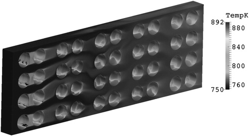
To conclude, it is clear that the flows under consideration through tube banks are especially complex, where even an idealized test case requires the use of especially demanding turbulence closures in the form of dynamic LES techniques to adequately reproduce the trends given by prior experimentation. However, computing power has not yet become so readily available that such a procedure is routine in industrial contexts, due to the ever-pressing need to obtain solutions in a practical and time-efficient manner. RANS-based methods will continue to dominate industrial applications for the foreseeable future, and indeed, remain the only viable option from this project’s perspective in further investigations involving a more representative geometry which is non-periodic. However, especially in the case of high-Re RANS turbulence models, the overly simplistic treatment of turbulent flow in the presence of bounding walls simply cannot adequately capture wall shear stresses and heat flux levels that are of primary interest to the work at large. Though the R_ij-ε SSG model returns acceptable static pressure levels and anticipates diagonalized flow, commensurate with experimental observations, the shortcomings of the thermal predictions in its current state must not be overlooked. The introduction of the Analytical Wall Function in Code_Saturne, whose near-wall momentum and thermal domains are shown under Figure 17, and its reproduction of both momentum and thermal logarithmic layers in agreement with Direct Numerical Simulation (DNS) data, shown under Figures 18 and 19, where the maximum percentage difference is on the order of 10% in both cases (improving to less than 5% as the boundary layer is traversed in the direction of increasing y*) demonstrate that it can at least in principle account for more elaborate near-wall turbulent flow phenomena without any major additional computational overhead. While this work is primarily targeting its utility in combination with the SSG second-moment closure model, it is being developed in tandem via the k-ε LP model for implementation testing purposes, and scope does exist for deriving an equivalent form for use in wall-modeled LES or hybrid RANS/LES approaches. It is clear, however, that further work is required to validate the AWF further, given the responses it has generated through use with the k-ε LP and R_ij-ε SSG models, where the improvements were neither unanimous nor confined to one particular model, rather, some aspects were improved for one model, and vice versa. Though not presented here, the true potential of the AWF is the ability to account for boundaries with augmented roughness, beyond the simplistic inclusion of an additive constant within the logarithm in the usual formulation. This approach considers the implications of near-wall roughness elements on impeding momentum in this region, as well as the gradual erosion of the viscous sublayer due to their presence. A “fully-rough” flow in a turbulent sense is one in which no laminar portion exists (due to the near-wall flow having been locally arrested by the elements, forming recirculation pockets) within the boundary layer and only turbulent effects prevail. Similarly, a thermal barrier is formed between the roughness elements, due to the locally reduced convection in this region. In cases of particulate build-up on working heat transfer surfaces, roughness acts to impede the amount of area that thermal energy flows through, so the problem is more associated with geometric considerations than the mismatch of thermal conductivities between the austenitic steel and carbon particulates, as this can occur well within the non-critical range of roughness height, namely at roughness levels before any perceptible effect on the momentum field occurs. Typically, roughness augmentation due to agglomeration of particles is only considered when the nascent geometry has features conducive to collecting them, e.g. ribs, channels, dimples, sharp corners, and so on. However, though the tubes considered in the secondary superheater platen of a serpentine AGR boiler system are not finned, the carburization process of steel at high temperatures in a carbon-rich environment entails the absorption of the particulates into the surface, where diffusion then takes place, leading to material property changes, concentrated at the boundary. Additionally, prolonged exposure also leads to the development of filaments which protrude from the surface, somewhat analogously to stalagmite formation on cave floors, which may then be broken off through shear or persist and grow enough in size to begin disrupting flow about the tubes. Depending on the extent of roughness overall, this may have the effect of inducing secondary swirling flows, which can limit the rate of convection through the array as a whole and further impede heat transfers. In summary, roughness is difficult to quantify in and of itself, and its effects on flows featuring heat transfers are multifaceted. Moreover, it could easily be envisaged that whatever effects are observed are case-dependent on the array in question, given the native complexity of smooth tube banks in the first instance. It is anticipated that the project will proceed along these lines at a later date. The geometry considered herein is somewhat atypical, as many applications involving bank of tubes tend to include finned surfaces to increase the effective working heat transfer area, unlike the smooth tubes considered here. However, the addition of surface fins leads to greater flow pressure losses through the array in general, meaning that a balance must be struck between ease of traversal for the working fluid in question and seeking greater heat transfer overall. For more information on this topic, the authors recommend the work by Wejkowski [31]. Early efforts have been made to assess the flow and heat transfer of a non-periodic platen consisting of 40 tubes and confining walls, as shown under Figure 20, with the intention of combining the above analysis with both smooth and rough-walled Analytical Wall Function formulations to inform EDF Energy’s safe plant lifetime extension scheme in the years to come.

Nomenclature
A	=	area through which flow navigates, m2
AGR	=	advanced gas-cooled reactor
AWF	=	analytical wall function
AU	=	constant handling near-wall normal velocity gradient, s−1
AΘ	=	constant handling near-wall normal temperature gradient, K m−1
BU	=	constant handing wall velocity value, m s−1
BΘ	=	constant handling wall temperature value, K
CPU	=	central processing unit
CU	=	near-wall momentum advection constant, kg s−2
CΘ	=	near-wall thermal advection constant, kg K m−1 s−1
C̅P	=	time and space-averaged static pressure coefficient
cp	=	specific heat capacity at constant pressure, J kg−1 K−1
C̅f	=	time and space-averaged friction coefficient
CL	=	lift coefficient
cL	=	near-wall equilibrium length-scale constant = 2.55
CD	=	drag coefficient
cμ	=	Eddy-diffusivity constant for a simple turbulent shear flow = 0.09
D	=	tube diameter, m
DNS	=	direct numerical simulation
f	=	elliptic relaxation function (as in the v̅2-f and φ-f turbulence models), or frequency of oscillation (as in the Strouhal number, fD/Ubulk), s−1
h	=	wall heat transfer coefficient, W m−2 K−1
k	=	turbulent kinetic energy per unit mass, m2 s−2
LP	=	linear production (as in the k−ε linear production turbulence model)
LES	=	Large Eddy Simulation
N	=	momentum advection at the near-wall cell’s North face, kg s−2
N̅u	=	time and space-averaged Nusselt number
P	=	pressure, Pa
PLEX	=	plant lifetime extension
$\overline{ P_k}$	=	averaged rate of turbulent kinetic energy production
PL	=	longitudinal tube pitch, m
PT	=	transverse tube pitch, m
Pr	=	molecular Prandtl number
Prt	=	turbulent Prandtl number (nominally 0.9 for fluids of Pr ≤ 1)
p	=	static pressure, Pa
p∞	=	freestream static pressure, Pa
Q	=	linear under-relaxation coefficient
qwall	=	wall heat flux, W m−2
RANS	=	Reynolds-averaged Navier–Stokes
Rij	=	Reynolds stress tensor
Re	=	Reynolds number
SSG	=	Speziale-Sarkar-Gatski (as in the Rij-ε SSG turbulence model)
SST	=	shear stress transport (as in the k−ω SST turbulence model)
St	=	Strouhal number
SΘ	=	thermal source term in energy equation (temperature in this case), kg K m−3 s−1
t	=	time
U	=	horizontal x-velocity (→ positive), m s−1
U*	=	normalized near-wall cell velocity
u̅v̅	=	component 1,2 of the Reynolds stress tensor, m2 s−2
V	=	vertical y-velocity (↑ positive), m s−1
v̅2	=	wall-normal component (2,2) of the Reynolds stress tensor, m2 s−2
x	=	fundamental horizontal Cartesian direction (→ positive), m
Y	=	near-wall turbulent eddy-viscosity scaling factor (up to cell node)
Yn	=	1 + α(${{\mathrm{y}}_{\mathrm{n}}^{\mathrm{*}}-\mathrm{y}}_{\mathrm{visc}}^{\mathrm{*}}$ ), whole boundary cell eddy-viscosity scaling factor
YΘn	=	1 + αΘ(${{\mathrm{y}}_{\mathrm{n}}^{\mathrm{*}}-\mathrm{y}}_{\mathrm{visc}}^{\mathrm{*}}$ ), thermal analog of Yn
y	=	fundamental Cartesian direction positive), m
yn	=	height of near-wall cell’s North face relative to boundary surface, m
y*	=	wall distance from node normalized by square root of turbulent kinetic energy
$y_{\mathit{visc}}^{*}$	=	dimensionless viscous (a.k.a. laminar) sublayer height
$y_{ϵ}^{*}$	=	dimensionless height of near-wall region where ε is deemed constant = 5.1
z	=	fundamental Cartesian direction concerning depth (ʘpositive), m

Greek symbols
Θ	=	temperature, K
Θ*	=	normalized near-wall cell temperature
α	=	product of cμ and cL used in near-wall eddy viscosity estimation
αΘ	=	αPr/Prt, thermal analog to α
β	=	pressure gradient, Pa m−1
γ	=	temperature gradient, K m−1
ε	=	rate of turbulent kinetic energy dissipation, m2 s−3
ε̅	=	averaged rate of turbulent kinetic energy dissipation, m2 s−3
θ	=	angle about tube surface, clockwise positive, zero at the leftmost point of the tube, °
λ	=	thermal conductivity, W m−1 K−1
μ	=	molecular dynamic viscosity, Pa s
μt	=	turbulent dynamic eddy viscosity, Pa s
ν	=	molecular kinematic viscosity, m2 s−1
νt	=	turbulent kinematic eddy viscosity, m2 s−1
ρ	=	density, kg m−3
τwall	=	wall shear stress, Pa
φ	=	normalized wall-normal component of the Reynolds stress tensor = v̅2/k
ω	=	turbulent frequency (a.k.a. specific dissipation) = ε/k, s−1

Subscripts
bulk	=	bulk quantity
gap	=	quantity evaluated at the location where spacing between tubes is minimized
L	=	longitudinal parameter
N	=	quantity evaluated at neighboring node immediately North of a near-wall cell
n	=	quantity evaluated at North face of near-wall cell
max	=	maximized quantity
min	=	minimized quantity
ref	=	reference or target value
perio	=	periodic component of quantity
T	=	transverse parameter
t	=	turbulent quantity
visc	=	quantity evaluated at the top of the viscous sublayer
wall	=	quantity evaluated at the solid boundary
Θ	=	thermal quantity
τ	=	quantity evaluated using friction velocity
∞	=	quantity evaluated under freestream conditions
1	=	near-wall quantity evaluated within the viscous sublayer
2	=	near-wall quantity evaluated above the viscous sublayer, subject to turbulent viscosity

Superscripts
n	=	time step
*	=	quantity normalized by square root of turbulent kinetic energy

Acknowledgements

The authors would like to acknowledge the assistance given by IT Services and the use of the Computational Shared Facility at The University of Manchester, and in addition, this work made use of the facilities of N8 HPC Centre of Excellence, provided and funded by the N8 consortium and EPSRC (Grant No. EP/K000225/1). The Centre is coordinated by the Universities of Leeds and Manchester.

Additional information

Notes on contributors

James L. Blackall

James L. Blackall graduated from the University of Manchester in 2014, where he read Aerospace Engineering. Currently he is undertaking a Ph.D. project in Nuclear Engineering within the Next Generation Nuclear Centre for Doctoral Training (NGN CDT) candidate under the direct supervision of Prof. Hector Iacovides and Dr. Juan Uribe, who fill the roles of academic and industrial advisors respectively. His research topic involves the study of complex turbulent flow phenomena about tube bank geometries of interest to EDF Energy, in support of its current policy of safe plant lifetime extensions.

Hector Iacovides

Hector Iacovides graduated from University College London in Mechanical Engineering, before joining the Thermo and Fluids Division of UMIST’s Mechanical Engineering Department firstly as a postgraduate student to obtain an M.Sc. degree in Thermodynamics and Fluid Mechanics, before completing a Ph.D. project in computational and experimental heat and fluid flow thereafter. He remained at UMIST’s Mechanical Engineering Department as a post-doctoral researcher initially, then later as a member of academic staff. Currently, he holds the Chair in Convective Heat Transfer at the University of Manchester’s School of Mechanical, Aerospace, and Civil Engineering (MACE). In June 2006, he shared the Award for Scientific Contribution from the Heat Transfer Society of Japan, with his two colleagues, Dr. T. J. Craft, also from the School of MACE, and Prof. K. Suga of Osaka Prefecture University.

Juan C. Uribe

Juan C. Uribe is a thermofluids research engineer at the EDF Energy R&D UK Centre. He gained his Ph.D. in turbulence modelling from the University of Manchester in 2006. He has worked in the nuclear industry for over 14 years in problems related to flow dynamics and heat transfer. He has been part of various consortia including European funded projects on high-resolution computational fluid dynamics. He currently works for the EDF Energy R&D UK Centre in the Low Carbon Generation team. He leads a team of engineers working in CFD as part of the Modelling and Simulation Centre. He works closely in projects related to Advanced Gas-Cooled Reactors in the UK and with the software development team in EDF R&D in France where he spent several months in training during the early 2000s.

Appendix:

Formulation of the analytical wall function of Suga et al. [18]

The full formulation and rationale behind the Analytical Wall Function is shown below, where the turbulent kinematic viscosity is as prescribed as defined in Eq. (10)(10) $${\mu }_t=\left\{\begin{array}{c} 0, \mathit{if} {\mathrm{y}}^{\mathrm{*}}<{\mathrm{y}}_{\mathrm{visc}}^{\mathrm{*}} \hfill \\ \mu c_{\mu }{c}_L\left(y^{\mathrm{*}}-y_{\mathit{visc}}^{\mathrm{*}}\right)= \mu \alpha \left(y^{\mathrm{*}}-y_{\mathit{visc}}^{\mathrm{*}}\right), \mathit{if} {\mathrm{y}}^{\mathrm{*}}\ge {\mathrm{y}}_{\mathrm{visc}}^{\mathrm{*}}\end{array}\right.\mathrm{ }$$(10) , where the constant α (= 0.2295) is the product of the eddy-diffusivity constant and the mixing-length hypothesis near-wall turbulent length scale constant c_L = 2.55. One may reasonably argue that all that has been achieved thus far is a change of one prescribed variable for another, from the mean flow velocity to turbulent viscosity, and thusly inquire as to what benefits this procedure can conceivably offer over the standard. The retort is that the assumption of a mean flow velocity profile (and indirectly, its gradient) based on largely outdated or case-specific reasoning leads to both mean velocity and turbulent viscosity being rigidly enforced in the near-wall region, where it cannot adapt based on local flow conditions, which may suffice for a channel flow, but has no guarantee of truly representing a real flow over complex geometry in a high-Re sense, over which a mean logarithmic layer need not exist at all. (10) $${\mu }_t=\left\{\begin{array}{c} 0, \mathit{if} {\mathrm{y}}^{\mathrm{*}}<{\mathrm{y}}_{\mathrm{visc}}^{\mathrm{*}} \hfill \\ \mu c_{\mu }{c}_L\left(y^{\mathrm{*}}-y_{\mathit{visc}}^{\mathrm{*}}\right)= \mu \alpha \left(y^{\mathrm{*}}-y_{\mathit{visc}}^{\mathrm{*}}\right), \mathit{if} {\mathrm{y}}^{\mathrm{*}}\ge {\mathrm{y}}_{\mathrm{visc}}^{\mathrm{*}}\end{array}\right.\mathrm{ }$$(10)

Figure 17 shows the near-wall domain used by the AWF for the momentum and thermal fields. The simplified boundary-layer Navier–Stokes equations subject to Assumptions A–D for near-wall momentum and thermal energy transport, shown as Eqs. (11)(11) $$\frac{\partial \left(\rho \mathit{UU}\right)}{\partial x}+\frac{\partial \left(\rho \mathit{VU}\right)}{\partial y}=-\frac{\partial P}{\partial x}+\frac{\partial }{\partial y}\left[\left(\mu +{\mu }_t\right)\frac{\partial U}{\partial y}\right]\mathrm{ }$$(11) and (12)(12) $$\frac{\partial \left(\rho U\mathrm{\Theta }\right)}{\partial x}+\frac{\partial \left(\rho V\mathrm{\Theta }\right)}{\partial y}=-S_{\mathrm{\Theta }}+\frac{\partial }{\partial y}\left[\left(\frac{\mu }{\mathit{Pr}}+\frac{{\mu }_t}{{\mathit{Pr}}_t}\right)\frac{\partial \mathrm{\Theta }}{\partial y}\right]\mathrm{ }$$(12) respectively, are rearranged for the terms C_U and C_Θ, denoting parallel near-wall convection for momentum and temperature correspondingly (deemed constant for each boundary cell), before converting the derivatives in the diffusion terms to refer to non-dimensional units of wall distance rather than physical distance between the near-wall cell’s node and its solid boundary, yielding Eqs. (13)(13) $$C_U=\frac{\partial }{\partial y^{\mathrm{*}}}\left[\left(\mu +{\mu }_t\right)\frac{\partial U}{\partial y^{\mathrm{*}}}\right]=\frac{{\nu }^2}{k_P}\left[\frac{\partial \left(\rho \mathit{UU}\right)}{\partial x}+\frac{\partial \left(\rho \mathit{VU}\right)}{\partial y}+\frac{\partial P}{\partial x}\right]\mathrm{ }$$(13) and (14)(14) $$C_{\mathrm{\Theta }}=\frac{\partial }{\partial {\mathrm{y}}^{\mathrm{*}}}\left[\left(\frac{\mu }{\mathit{Pr}}+\frac{{\mu }_t}{{\mathit{Pr}}_t}\right)\frac{\partial \mathrm{\Theta }}{\partial y^{\mathrm{*}}}\right]=\mathrm{ }\frac{{\nu }^2}{k_P}\left[\frac{\partial \left(\rho U\mathrm{\Theta }\right)}{\partial x}+\frac{\partial \left(\rho V\mathrm{\Theta }\right)}{\partial y}+S_{\mathrm{\Theta }}\right]\mathrm{ }$$(14) . (11) $$\frac{\partial \left(\rho \mathit{UU}\right)}{\partial x}+\frac{\partial \left(\rho \mathit{VU}\right)}{\partial y}=-\frac{\partial P}{\partial x}+\frac{\partial }{\partial y}\left[\left(\mu +{\mu }_t\right)\frac{\partial U}{\partial y}\right]\mathrm{ }$$(11) (12) $$\frac{\partial \left(\rho U\mathrm{\Theta }\right)}{\partial x}+\frac{\partial \left(\rho V\mathrm{\Theta }\right)}{\partial y}=-S_{\mathrm{\Theta }}+\frac{\partial }{\partial y}\left[\left(\frac{\mu }{\mathit{Pr}}+\frac{{\mu }_t}{{\mathit{Pr}}_t}\right)\frac{\partial \mathrm{\Theta }}{\partial y}\right]\mathrm{ }$$(12) (13) $$C_U=\frac{\partial }{\partial y^{\mathrm{*}}}\left[\left(\mu +{\mu }_t\right)\frac{\partial U}{\partial y^{\mathrm{*}}}\right]=\frac{{\nu }^2}{k_P}\left[\frac{\partial \left(\rho \mathit{UU}\right)}{\partial x}+\frac{\partial \left(\rho \mathit{VU}\right)}{\partial y}+\frac{\partial P}{\partial x}\right]\mathrm{ }$$(13) (14) $$C_{\mathrm{\Theta }}=\frac{\partial }{\partial {\mathrm{y}}^{\mathrm{*}}}\left[\left(\frac{\mu }{\mathit{Pr}}+\frac{{\mu }_t}{{\mathit{Pr}}_t}\right)\frac{\partial \mathrm{\Theta }}{\partial y^{\mathrm{*}}}\right]=\mathrm{ }\frac{{\nu }^2}{k_P}\left[\frac{\partial \left(\rho U\mathrm{\Theta }\right)}{\partial x}+\frac{\partial \left(\rho V\mathrm{\Theta }\right)}{\partial y}+S_{\mathrm{\Theta }}\right]\mathrm{ }$$(14)

These equations are then integrated twice to obtain equations for the near-wall velocity and temperature, dependent on whether or not the near-wall node lies within the viscous sublayer (whose height is prescribed as 10.88) or above it in either the buffer or logarithmic zones, giving Eqs. (15)(15) $$U=\left\{\begin{array}{c} \frac{C_{U_1}}{2\mu }{y}^{\mathrm{*}2}+\frac{A_{U_1}}{\mu }{y}^{\mathrm{*}}+\frac{B_{U_1}}{\mu }, \mathit{if} {\mathrm{y}}^{\mathrm{*}}<{\mathrm{y}}_{\mathrm{visc}}^{\mathrm{*}}=10.88\hfill \\ \frac{C_{U_2}}{\alpha \mu }\left[y^{\mathrm{*}}-\left(\frac{1}{\alpha }-y_{\mathit{visc}}^{\mathrm{*}}\right)\ln Y\right]+\frac{A_{U_2}}{\alpha \mu }\ln Y+\frac{B_{U_2}}{\mu }, \mathrm{if} {\mathrm{y}}^{\mathrm{*}}\ge {\mathrm{y}}_{\mathrm{visc}}^{\mathrm{*}}=10.88\end{array}\right.\mathrm{ }$$(15) and (16)(16) $$\mathrm{\Theta }=\left\{\begin{array}{c}\frac{\mathit{Pr}{C}_{{\mathrm{\Theta }}_1}}{2\mu }{y}^{\mathrm{*}2}+\frac{\mathit{Pr}{A}_{\mathrm{\Theta }}}{\mu }{y}^{\mathrm{*}}+B_{{\mathrm{\Theta }}_1}, \mathit{if} {\mathrm{y}}^{\mathrm{*}}<{\mathrm{y}}_{\mathrm{visc}}^{\mathrm{*}}\hfill \\ \frac{\mathit{Pr}{C}_{{\mathrm{\Theta }}_2}}{{\alpha }_{\mathrm{\Theta }}\mu }\left(y^{\mathrm{*}}-y_{\mathit{visc}}^{\mathrm{*}}\right)+\frac{\mathit{Pr}}{{\alpha }_{\mathrm{\Theta }}\mu }\left(A_{\mathrm{\Theta }}+C_{{\mathrm{\Theta }}_1}{y}_{\mathit{visc}}^{\mathrm{*}}-\frac{C_{{\mathrm{\Theta }}_2}}{{\alpha }_{\mathrm{\Theta }}}\right)\ln Y_{\mathrm{\Theta }}+B_{{\mathrm{\Theta }}_2}, \mathit{if} {\mathrm{y}}^{\mathrm{*}}\ge {\mathrm{y}}_{\mathrm{visc}}^{\mathrm{*}}\end{array}\right.\mathrm{ }$$(16) . Note that the values of C_U and C_Θ also exhibit dependence on the normal distance of the near-wall node, due to μ_t being zero in the viscous sublayer. Hereafter, any quantities featuring a subscript of “1” are evaluated in the laminar region, while those with a “2” subscript take the effects of turbulent viscosity into account, following the notation of Gerasimov [28]. (15) $$U=\left\{\begin{array}{c} \frac{C_{U_1}}{2\mu }{y}^{\mathrm{*}2}+\frac{A_{U_1}}{\mu }{y}^{\mathrm{*}}+\frac{B_{U_1}}{\mu }, \mathit{if} {\mathrm{y}}^{\mathrm{*}}<{\mathrm{y}}_{\mathrm{visc}}^{\mathrm{*}}=10.88\hfill \\ \frac{C_{U_2}}{\alpha \mu }\left[y^{\mathrm{*}}-\left(\frac{1}{\alpha }-y_{\mathit{visc}}^{\mathrm{*}}\right)\ln Y\right]+\frac{A_{U_2}}{\alpha \mu }\ln Y+\frac{B_{U_2}}{\mu }, \mathrm{if} {\mathrm{y}}^{\mathrm{*}}\ge {\mathrm{y}}_{\mathrm{visc}}^{\mathrm{*}}=10.88\end{array}\right.\mathrm{ }$$(15) (16) $$\mathrm{\Theta }=\left\{\begin{array}{c}\frac{\mathit{Pr}{C}_{{\mathrm{\Theta }}_1}}{2\mu }{y}^{\mathrm{*}2}+\frac{\mathit{Pr}{A}_{\mathrm{\Theta }}}{\mu }{y}^{\mathrm{*}}+B_{{\mathrm{\Theta }}_1}, \mathit{if} {\mathrm{y}}^{\mathrm{*}}<{\mathrm{y}}_{\mathrm{visc}}^{\mathrm{*}}\hfill \\ \frac{\mathit{Pr}{C}_{{\mathrm{\Theta }}_2}}{{\alpha }_{\mathrm{\Theta }}\mu }\left(y^{\mathrm{*}}-y_{\mathit{visc}}^{\mathrm{*}}\right)+\frac{\mathit{Pr}}{{\alpha }_{\mathrm{\Theta }}\mu }\left(A_{\mathrm{\Theta }}+C_{{\mathrm{\Theta }}_1}{y}_{\mathit{visc}}^{\mathrm{*}}-\frac{C_{{\mathrm{\Theta }}_2}}{{\alpha }_{\mathrm{\Theta }}}\right)\ln Y_{\mathrm{\Theta }}+B_{{\mathrm{\Theta }}_2}, \mathit{if} {\mathrm{y}}^{\mathrm{*}}\ge {\mathrm{y}}_{\mathrm{visc}}^{\mathrm{*}}\end{array}\right.\mathrm{ }$$(16)

The A_U, A_Θ, B_U, and B_Θ constants within the expressions for velocity and temperature are determined by equating the gradients and values obtained by both the laminar sublayer and turbulence-affected equations, in addition to applying boundary conditions, in order to ensure a smooth and continuous transition between laminar and turbulent portions of near-wall flow, wherever the near-wall node is deemed to lie in non-dimensional units. In the case of stationary walls, B_U is zero due to the no-slip condition. U_n, the equivalent velocity value at the North face of a near-wall cell, is determined by linear interpolation between a boundary node and its northern neighbor. (17) $$A_U=\left\{\begin{array}{c} \frac{\mu U_n-N}{\left[\frac{\ln Y_n}{\alpha }+y_{\mathit{visc}}^{\mathrm{*}}\right]}, \mathrm{if} {\mathrm{y}}^{\mathrm{*}}<{\mathrm{y}}_{\mathrm{visc}}^{\mathrm{*}} \hfill \\ \left(C_{U_1}-C_{U_2}\right)y_{\mathit{visc}}^{\mathrm{*}}+ \frac{\mu U_n-N}{\left[\frac{\ln Y_n}{\alpha }+y_{\mathit{visc}}^{\mathrm{*}}\right]}, \mathit{if} {\mathrm{y}}^{\mathrm{*}}\ge {\mathrm{y}}_{\mathrm{visc}}^{\mathrm{*}}\end{array}\right.\mathrm{ }$$(17) (18) $$B_U=\mathrm{ }\left\{\begin{array}{c}{\mathrm{ }U}_{\mathit{wall}} \left(=0\text{ for stationary walls}\right), \mathrm{if} {\mathrm{y}}^{\mathrm{*}}<{\mathrm{y}}_{\mathrm{visc}}^{\mathrm{*}}\\ y_{\mathit{visc}}^{\mathrm{*}}\left(\frac{C_{U_1}}{2}{y}_{\mathit{visc}}^{\mathrm{*}}-\frac{C_{U_2}}{\alpha }+A_{U_1}\right), \mathrm{if}{\text{ y}}^{\mathrm{*}}\ge {\mathrm{y}}_{\mathrm{visc}}^{\mathrm{*}}\end{array}\mathrm{ }\right.$$(18) (19) $$A_{\mathrm{\Theta }}=\mathrm{ }\left\{\begin{array}{c}\frac{q_{\mathit{wall}}}{c_p}\frac{\mu }{\rho \sqrt{k_P}}, \mathit{for} \mathit{wall} \mathit{isoflux} \mathit{boundary} \mathit{conditions}\hfill \\ \frac{\left({\mathrm{\Theta }}_n-{\mathrm{\Theta }}_{\mathit{wall}}\right)\frac{\mu }{\mathit{Pr}}-\frac{1}{{\alpha }_{\mathrm{\Theta }}}\left[C_{{\mathrm{\Theta }}_1}{y}_{\mathit{visc}}^{\mathrm{*}}-\frac{C_{{\mathrm{\Theta }}_2}}{{\alpha }_{\mathrm{\Theta }}}\right]\ln Y_{{\mathrm{\Theta }}_n}-\frac{C_{{\mathrm{\Theta }}_1}}{2}{y}_{\mathit{visc}}^{{\mathrm{*}}^2}}{\frac{1}{{\alpha }_{\mathrm{\Theta }}}{Y}_{{\mathrm{\Theta }}_n}+y_{\mathit{visc}}^{\mathrm{*}}}, \mathit{Isothermal} \mathit{walls}\end{array}\mathrm{ }\right.$$(19) (20) $$B_{\mathrm{\Theta }}=\mathrm{ }\left\{\begin{array}{c}{\mathrm{\Theta }}_{\mathit{wall}}, \mathit{if} {\mathrm{y}}^{\mathrm{*}}<{\mathrm{y}}_{\mathrm{visc}}^{\mathrm{*}} \hfill \\ \frac{\mathit{Pr}{y}_{\mathit{visc}}^{\mathrm{*}}}{\mu }\left[\frac{C_{{\mathrm{\Theta }}_1}{y}_{\mathit{visc}}^{\mathrm{*}}}{2}+A_{\mathrm{\Theta }}\right]+{\mathrm{\Theta }}_{\mathit{wall}}, \mathit{if} {\mathrm{y}}^{\mathrm{*}}\ge {\mathrm{y}}_{\mathrm{visc}}^{\mathrm{*}}\end{array}\mathrm{ }\right.$$(20) (21) $$N=\frac{C_{U_2}}{\alpha }\left[y_n^{\mathrm{*}}-\left(\frac{1}{\alpha }-y_{\mathit{visc}}^{\mathrm{*}}\right)\ln Y_n\right]+\frac{C_{U_1}-C_{U_2}}{\alpha }{y}_{\mathit{visc}}^{\mathrm{*}}\ln Y_n+\left(\frac{C_{U_1}}{2}{y}_{\mathit{visc}}^{\mathrm{*}}-\frac{C_{U_2}}{\alpha }\right)y_{\mathit{visc}}^{\mathrm{*}}\mathrm{ }$$(21)

In the event that uniform wall heat flux conditions are prescribed, Eq. (22)(22) $${\mathrm{\Theta }}_{\mathit{wall}}=\mathrm{ }{\mathrm{\Theta }}_n-\frac{\mathit{Pr}}{\mu }\left[\frac{C_{{\mathrm{\Theta }}_2}}{{\alpha }_{\mathrm{\Theta }}}\left(y_n^{\mathrm{*}}-y_{\mathit{visc}}^{\mathrm{*}}\right)+\frac{\ln Y_{{\mathrm{\Theta }}_n}}{{\alpha }_{\mathrm{\Theta }}}\left(A_{\mathrm{\Theta }}+C_{{\mathrm{\Theta }}_1}{y}_{\mathit{visc}}^{\mathrm{*}}-\frac{C_{{\mathrm{\Theta }}_2}}{{\alpha }_{\mathrm{\Theta }}}\right)+y_{\mathit{visc}}^{\mathrm{*}}\left(A_{\mathrm{\Theta }}+\frac{C_{{\mathrm{\Theta }}_1}{y}_{\mathit{visc}}^{\mathrm{*}}}{2}\right)\right)]\mathrm{ }$$(22) documents the required relationship for wall temperature, where Θ_n is determined using interpolation similar to U_n, but in the thermal domain: (22) $${\mathrm{\Theta }}_{\mathit{wall}}=\mathrm{ }{\mathrm{\Theta }}_n-\frac{\mathit{Pr}}{\mu }\left[\frac{C_{{\mathrm{\Theta }}_2}}{{\alpha }_{\mathrm{\Theta }}}\left(y_n^{\mathrm{*}}-y_{\mathit{visc}}^{\mathrm{*}}\right)+\frac{\ln Y_{{\mathrm{\Theta }}_n}}{{\alpha }_{\mathrm{\Theta }}}\left(A_{\mathrm{\Theta }}+C_{{\mathrm{\Theta }}_1}{y}_{\mathit{visc}}^{\mathrm{*}}-\frac{C_{{\mathrm{\Theta }}_2}}{{\alpha }_{\mathrm{\Theta }}}\right)+y_{\mathit{visc}}^{\mathrm{*}}\left(A_{\mathrm{\Theta }}+\frac{C_{{\mathrm{\Theta }}_1}{y}_{\mathit{visc}}^{\mathrm{*}}}{2}\right)\right)]\mathrm{ }$$(22)

Finally, Eqs. (23)(23) $$\overline{P_k}=\left\{\begin{array}{c}0, \mathrm{if} {\mathrm{y}}^{\mathrm{*}}<{\mathrm{y}}_{\mathrm{visc}}^{\mathrm{*}}\hfill \\ -\frac{1}{y_n}\int \overline{\mathit{uv}}\frac{\partial U}{\partial y}dy\mathrm{ }=\frac{1}{y_n}\frac{\rho \sqrt{k_P}}{\mu } {\int }_{y_{\mathit{visc}}^{\mathrm{*}}}^{y_n^{\mathrm{*}}}\mu \alpha \left(y^{\mathrm{*}}-y_{\mathit{visc}}^{\mathrm{*}}\right){\left(\frac{\partial U_2}{\partial y^{\mathrm{*}}}\right)}^{2}d{y}^{\mathrm{*}}, \mathit{if} {\mathrm{y}}^{\mathrm{*}}\ge {\mathrm{y}}_{\mathrm{visc}}^{\mathrm{*}}\end{array}\mathrm{ }\right.$$(23) and (24)(24) $$\overline{\epsilon }=\mathrm{ }\left\{\begin{array}{c}\frac{2k_P^2}{\nu y_{\epsilon }^{{\mathrm{*}}^2}}, \mathit{if} {\mathrm{y}}_{\mathrm{\epsilon }}^{\mathrm{*}}=5.1>{\mathrm{y}}_{\mathrm{n}}^{\mathrm{*}} \hfill \\ \frac{k_P^2}{\nu y_n^{\mathrm{*}}\mathrm{ }}\left[\frac{2}{y_{\epsilon }^{\mathrm{*}}}\left(1+\ln \left(\frac{y_n^{\mathrm{*}}}{y_{\epsilon }^{\mathrm{*}}}\right)\right)\right], \mathit{if} {\mathrm{y}}_{\mathrm{\epsilon }}^{\mathrm{*}}=5.1\le {\mathrm{y}}_{\mathrm{n}}^{\mathrm{*}}\end{array}\mathrm{ }\right.$$(24) describe how the turbulent production and dissipation rate quantities are handled in the near-wall cells, where the integral in the production term is estimated numerically via the trapezoidal rule to give the average value in the near-wall cell necessary for solution of the turbulent kinetic energy transport equation. The value taken by the averaged turbulent kinetic energy dissipation rate varies dependent on the height of the boundary cell, where $y_{\mathrm{\epsilon }}^{\mathrm{*}}$ is a constant value equal to double that of the equilibrium length scale constant, c_L = 2.55. DNS data suggest that the value of ε is fairly constant within the laminar sublayer below y* = 5.1, and increases logarithmically with increasing distance from the wall, where the corresponding formulations under Eq. (24)(24) $$\overline{\epsilon }=\mathrm{ }\left\{\begin{array}{c}\frac{2k_P^2}{\nu y_{\epsilon }^{{\mathrm{*}}^2}}, \mathit{if} {\mathrm{y}}_{\mathrm{\epsilon }}^{\mathrm{*}}=5.1>{\mathrm{y}}_{\mathrm{n}}^{\mathrm{*}} \hfill \\ \frac{k_P^2}{\nu y_n^{\mathrm{*}}\mathrm{ }}\left[\frac{2}{y_{\epsilon }^{\mathrm{*}}}\left(1+\ln \left(\frac{y_n^{\mathrm{*}}}{y_{\epsilon }^{\mathrm{*}}}\right)\right)\right], \mathit{if} {\mathrm{y}}_{\mathrm{\epsilon }}^{\mathrm{*}}=5.1\le {\mathrm{y}}_{\mathrm{n}}^{\mathrm{*}}\end{array}\mathrm{ }\right.$$(24) give a continuous and smooth variation of ε. (23) $$\overline{P_k}=\left\{\begin{array}{c}0, \mathrm{if} {\mathrm{y}}^{\mathrm{*}}<{\mathrm{y}}_{\mathrm{visc}}^{\mathrm{*}}\hfill \\ -\frac{1}{y_n}\int \overline{\mathit{uv}}\frac{\partial U}{\partial y}dy\mathrm{ }=\frac{1}{y_n}\frac{\rho \sqrt{k_P}}{\mu } {\int }_{y_{\mathit{visc}}^{\mathrm{*}}}^{y_n^{\mathrm{*}}}\mu \alpha \left(y^{\mathrm{*}}-y_{\mathit{visc}}^{\mathrm{*}}\right){\left(\frac{\partial U_2}{\partial y^{\mathrm{*}}}\right)}^{2}d{y}^{\mathrm{*}}, \mathit{if} {\mathrm{y}}^{\mathrm{*}}\ge {\mathrm{y}}_{\mathrm{visc}}^{\mathrm{*}}\end{array}\mathrm{ }\right.$$(23) (24) $$\overline{\epsilon }=\mathrm{ }\left\{\begin{array}{c}\frac{2k_P^2}{\nu y_{\epsilon }^{{\mathrm{*}}^2}}, \mathit{if} {\mathrm{y}}_{\mathrm{\epsilon }}^{\mathrm{*}}=5.1>{\mathrm{y}}_{\mathrm{n}}^{\mathrm{*}} \hfill \\ \frac{k_P^2}{\nu y_n^{\mathrm{*}}\mathrm{ }}\left[\frac{2}{y_{\epsilon }^{\mathrm{*}}}\left(1+\ln \left(\frac{y_n^{\mathrm{*}}}{y_{\epsilon }^{\mathrm{*}}}\right)\right)\right], \mathit{if} {\mathrm{y}}_{\mathrm{\epsilon }}^{\mathrm{*}}=5.1\le {\mathrm{y}}_{\mathrm{n}}^{\mathrm{*}}\end{array}\mathrm{ }\right.$$(24)

Figures 18 and 19 show the performance of the AWF over a simple channel flow in capturing the momentum and thermal boundary layers near a hydraulically smooth wall with the k − ε LP and R_ij-ε SSG models, compared with DNS data for cases of Re_τ = 395 [29] and 950 [30], where the former case also has available data for various Prandtl numbers (albeit all below unity), allowing for comparisons to be made with data on different thermal boundary layer thicknesses. It can be seen immediately that good agreement has been achieved using both high-Re models at both Reynolds numbers and all Prandtl numbers considered. Other modifications to the scheme can be employed that account for the effects of boundary layer accelerations on the viscous sublayer height, but these have yet to be implemented.

Figure 1. Square and triangular primitive units for banks of tubes, corresponding to in-line (left) and staggered (right) banks.

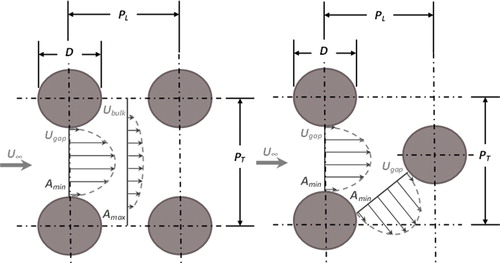
Figure 2. Sketch adapted from [6] with permission, showing three of the five flow patterns typically exhibited by in-line tube banks with variable longitudinal ($\frac{P_T}{D}$) and transverse pitches ($\frac{P_L}{D}$), where the shaded section indicates an impossible arrangement.

Figure 3. Meshes used for the periodic tube domain, representing an indefinite square in-line tube bank with pitch-to-diameter ratio equal to 1.6.

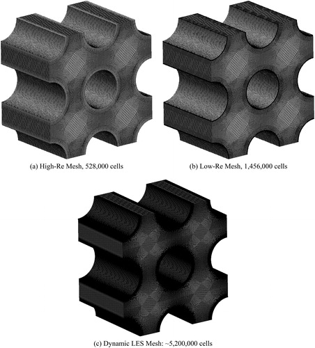
Figure 4. Plots showing mesh insensitivity using the k-ω SST model at resolutions of 4, 8, 16, and 20 spanwise cells per tube diameter in length, with corresponding cell counts of 291,200, 582,400, 1,164,800, and 1,456,000, compared to Aiba et al. [17] and West [4].

Figure 5. Plot demonstrating the convergence of the simulation toward the desired Reynolds number in time, where time-averaging begins once the variable Reynolds number reaches to within ±10 of the target.

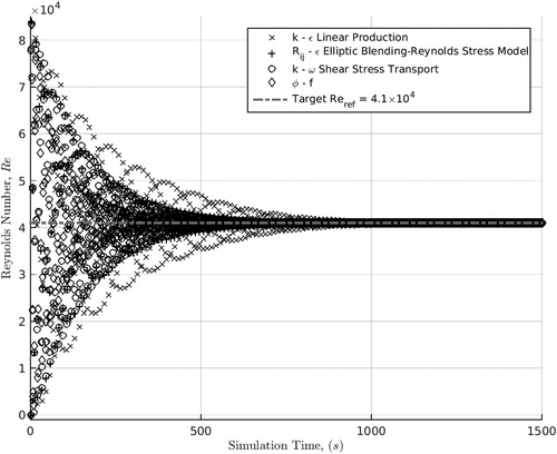
Figure 6. Plot showing the periodicity of the fluctuating lift and drag coefficient signals behind the central tube of the flow domain using the R_ij-ε SSG model, indicating that periodic conditions are reached that are appropriate for time and spatial averaging.

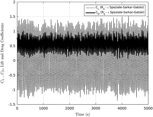
Figure 7. Plot showing the Fast Fourier Transform of the lift signal under Fig. 6, indicating that the dominant Strouhal number is ∼0.162 (St = fD/U_bulk), equivalent to a frequency of 2.458 Hz, where time-averaging takes place for all following results over 3,500 s of simulation time.

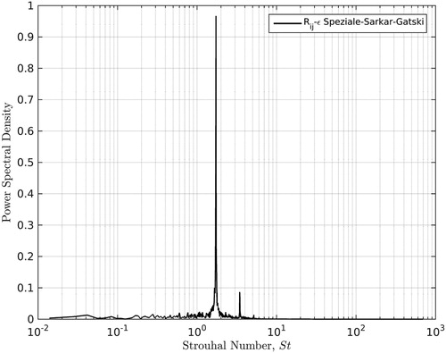
Figure 8. Plot showing the time-averaged static pressure coefficient distribution about the central tube in the three-dimensional 2 × 2 periodic array, as obtained by the low-Reynolds number turbulence models tested, compared with the experimental data of Aiba et al. [17].

Figure 9. Plot showing the time-averaged static pressure coefficient distribution about the central tube in the three-dimensional 2 × 2 periodic array, as obtained by the k-ε LP turbulence model using the standard wall function and the AWF [18], and Dynamic LES, compared with the data of Aiba et al. [17].

Figure 10. Plot showing the time-averaged static pressure coefficient distribution about the central tube in the three-dimensional 2 × 2 periodic array, as obtained by the R_ij-ε SSG turbulence model using the standard wall function and the AWF [18], and Dynamic LES, compared with the data of Aiba et al. [17].

Figure 11. Plot showing the time-averaged Nusselt number distribution about the central tube in the three-dimensional 2 × 2 periodic array, as obtained by the low-Reynolds number turbulence models tested, compared with the heat transfer data of Aiba et al. [17].

Figure 12. Plot showing the time-averaged Nusselt number distribution about the central tube in the three-dimensional 2 × 2 periodic array, as obtained by the k-ε LP turbulence model using the standard wall function and the AWF [18], and Dynamic LES, compared with the heat transfer data of Aiba et al. [17].

Figure 13. Plot showing the time-averaged Nusselt number distribution about the central tube in the three-dimensional 2 × 2 periodic array, as obtained by the R_ij-ε SSG turbulence model using the standard wall function and the AWF [18], and Dynamic LES, compared with the heat transfer data of Aiba et al. [17].

Figure 14. Plot showing the time-averaged friction coefficient distribution about the central tube in the three-dimensional 2 × 2 periodic array, as obtained by the low-Reynolds turbulence models tested against the prediction made via Dynamic LES.

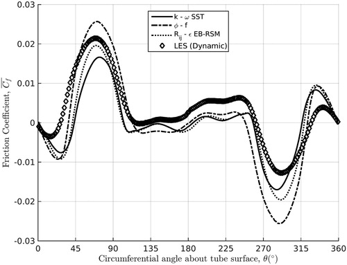
Figure 15. Plot showing the time-averaged friction coefficient distribution about the central tube in the three-dimensional 2 × 2 periodic array, as obtained by the k-ε LP turbulence model using the standard wall function and the AWF [18] against the prediction made via Dynamic LES.

Figure 16. Plot showing the time-averaged friction coefficient distribution about the central tube in the three-dimensional 2 × 2 periodic array, as obtained by the R_ij-ε LP turbulence model using the standard wall function and the AWF [18] against the prediction made via Dynamic LES.

Figure 17. Diagrams representing the momentum (left) and thermal (right) domains considered by the smooth-walled Analytical Wall Function on a cell-by-cell basis in the near-wall region of flow.

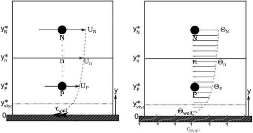
Figure 18. Plot showing the close agreement between the Analytical Wall Function and DNS data for a statistically-steady, two-dimensional turbulent momentum boundary layer in a channel flow at Re_τ = 395 [29] and Re_τ = 950 [30].

Figure 19. Plot showing the close agreement between the Analytical Wall Function and DNS data for a statistically-steady, two-dimensional turbulent thermal boundary layer in a channel flow at Re_τ = 395 at various Prandtl numbers [29].

Figure 20. Filled thermal contours showing a snapshot of the unsteady left-to-right flow in a non-periodic 40-tube platen subject to confining walls, calculated using N8 HPC resources on a block-structured mesh numbering ∼9.8 M cells using the k-ε LP turbulence model in Code_Saturne.

References

- D. Linton and B. Thornber, “Direct numerical simulation of transitional flow in a staggered tube bundle,” Phys. Fluids, vol. 28, no. 2, pp. 024111, 2016. DOI: 10.1063/1.4942180.
- E.D.F. Energy, “A new lease of life”. [Online]. Available: https://www.edfenergy.com/about/climate-change-solutions/plex.
- E. Nonbøl, “Description of the advanced gas cooled type of reactor (AGR), Risø National Laboratory, Roskilde, Denmark.” [Online]. Available: http://www.iaea.org/inis/collection/NCLCollectionStore/_Public/28/028/28028509.pdf.
- A. West, “Assessment of computational strategies for modelling in-line tube banks”, Ph.D. thesis, The University of Manchester, 2013
- E. Achenbach, “Heat transfer from smooth and rough in-line tube banks at high Reynolds number,” Int. J. Heat Mass Transfer, vol. 34, no. 1, pp. 152–155, Feb. 1971. DOI: 10.1016/0017-9310(91)90186-I.
- S. Ishigai and E. Nishikawa, “Structure of gas flow and its pressure loss in tube banks with tube axes normal to flow,” Trans. JSME, vol. 43, no. 373, pp. 3310–3319, 1977. DOI: 10.1299/kikai1938.43.3310.
- P. Moretti, “Flow-induced vibrations in arrays of cylinders,” Annu. Rev. Fluid Mech., vol. 25, no. 1, pp. 99–114, 1993. DOI: 10.1146/annurev.fl.25.010193.000531.
- I. Afgan, Y. Kahil, S. Benhamadouche, and P. Sagaut, “Large eddy simulation of the flow around single and two side-by-side cylinders at subcritical Reynolds numbers,” Phys. Fluids, vol. 23, no. 7, pp. 075101–075101, 2011. DOI: 10.1063/1.3596267.
- S. S. Chen. “Flow-induced vibration of circular cylindrical structures”, Argonne National Lab. (ANL), no. ANL-85-51, pp. 418–461, 1985.
- S. Ziada, “Vorticity shedding and acoustic resonance in tube bundles,” J. Braz. Soc. Mech. Sci. Eng., vol. 28, no. 2, pp. 186–199, 2006. DOI: 10.1590/S1678-58782006000200008.
- S. Acharya, S. Dutta, T. A. Myrum, and R. S. Baker, “Periodically developed flow and heat transfer in a ribbed duct,” Int. J. Heat Mass Transfer, vol. 36, no. 8, pp. 2069–2082, 1993. DOI: 10.1016/S0017-9310(05)80138-3.
- F. Archambeau, N. Méchitoua, and M. Sakiz, “Code saturne: a finite volume code for the computation of turbulent incompressible flows – industrial applications,” Int. J. Finite Volumes, vol. 1, no. 1, pp. 1–62, 2004.
- W. P. Jones and B. E. Launder, “The prediction of laminarization with a 2-equation model of turbulence,” Int. J. Heat Mass Transfer, vol. 15, no. 2, pp. 301–314, Feb. 1972. DOI: 10.1016/0017-9310(72)90076-2.
- R. Manceau, “Recent progress in the development of the Elliptic Blending Reynolds-stress model,” Int. J. Heat Fluid Flow, vol. 51, pp. 195–220, Feb. 2015. DOI: 10.1016/j.ijheatfluidflow.2014.09.002.
- J. Smagorinsky, “General circulation experiments with the primitive equations,” Mon. Weather Rev., vol. 91, no. 3, pp. 99–164, Mar. 1963. DOI: 10.1175/1520-0493(1963)091 < 009:GCEWTP>2.3.CO;2.
- M. Germano, U. Piomelli, P. Moin, and W. Cabot, “A dynamic subgrid-scale eddy viscosity model,” Phys. Fluids, vol. 3, no. 7, pp. 1760–1765, 1991. DOI: 10.1063/1.857955.
- S. Aiba, H. Tsuchida, and T. Ota, “Heat transfer around tubes in inline tube banks,” Bull. JSME, vol. 25, no. 204, pp. 919–924, Jun. 1982. DOI: 10.1299/jsme1958.25.919.
- K. Suga, T. J. Craft, and H. Iacovides, “An analytical wall-function for turbulent flows and heat transfer over rough walls,” Int. J. Heat Fluid Flow, vol. 27, no. 5, pp. 852–866, 2006. DOI: 10.1016/j.ijheatfluidflow.2006.03.011.
- H. Blasius, “Boundary layers in fluids of small viscosity,” Z. Math. Physik, vol. 56, no. 1, pp. 1–37, 1908.
- V. Guimet and D. R. Laurence, “A linearised turbulent production in the k-ε model for engineering applications”, presented at the 5th Engineering Turbulence Modelling and Measurements conference, Mallorca, Spain, December 2002, DOI: 10.1016/B978-008044114-6/50014-4.
- F. R. Menter, “Two-equation eddy-viscosity turbulence models for engineering applications,” Am. Inst. Aeronaut. Astronaut., vol. 32, no. 8, pp. 1598–1605, 1994. DOI: 10.2514/3.12149.
- D. R. Laurence, J. C. Uribe, and S. V. Utyuzhnikov, “A robust formulation of the v̅2-f model,” Flow Turbul. Combust., vol. 73, no. 3-4, pp. 169–185, 2005. DOI: 10.1007/s10494-005-1974-8.
- P. Durbin, “Near-wall turbulence closure modelling without “damping functions,” Theor. Comp. Fluid Dyn., vol. 3, no. 1, pp. 1–13, 1991. DOI: 10.1007/BF00271513.
- C. G. Speziale, S. Sarkar, and T. B. Gatski, “Modelling the pressure-strain correlation of turbulence: an invariant dynamical systems approach,” J. Fluid Mech., vol. 227, pp. 245–272, Jun. 1991. DOI: 10.1017/S002211209100101.
- R. Manceau, and K. Hanjalić, “Elliptic blending model: a new near-wall Reynolds-stress turbulence closure,” Phys. Fluids, vol. 14, no. 2, pp. 744–754, 2002. DOI: 10.1063/1.1432693.
- B. E. Launder, and D. B. Spalding, “The numerical computation of turbulent flows,” Comput. Methods Appl. Mech. Eng., vol. 3, no. 2, pp. 269–289, 1974. DOI: 10.1016/0045-7825(74)90029-2.
- V. S. Arpaci and P. S. Larsen. Convection Heat Transfer. New York: Prentice Hall, 1984.
- A. Gerasimov, “Development and validation of an analytical wall function strategy for modeling forced, mixed and natural convection flows”, Ph.D. thesis, University of Manchester, 2003
- H. Kawamura, H. Abe, and Y. Matsuo, “DNS of turbulent heat transfer in channel flow with respect to Reynolds and Prandtl number effects,” Int. J. Heat Fluid Flow, vol. 20, no. 3, pp. 196–207, 1999. DOI: 10.1016/S0142-727X(99)00014-4.
- S. Hoyas and J. Jiménez, “Reynolds number effects on the Reynolds-stress budgets in turbulent channels,” Phys. Fluids, vol. 20, no. 10, pp. 101511, 2008. DOI: 10.1063/1.3005862.
- R. Wejkowski, “Heat transfer and pressure loss in combined tube banks with triple-finned tubes,” Heat Transfer Eng., vol. 37, no. 1, pp. 45–52, 2016.DOI: 10.1080/01457632.2015.1042336.