Organic Matter Degradation in Energy-Limited Subsurface Environments—A Bioenergetics-Informed Modeling Approach

Abstract

Microbial degradation of organic matter is a key driver of subsurface biogeochemistry. Here, we present a bioenergetics-informed kinetic model for the anaerobic degradation of macromolecular organic matter that accounts for extracellular hydrolysis, fermentation, and respiration. The catabolic energy generated by fermentation and respiration is allocated to biomass growth, production of extracellular hydrolytic enzymes, and cellular maintenance. Microbial cells are assumed to exist in active or dormant states with marked differences in maintenance energy requirements. Dormant cells are further assumed to fulfill their maintenance energy requirements by utilizing their own biomass instead of relying on external substrates. When the catabolic Gibbs energy production for a given functional group of microorganisms exceeds the total maintenance energy requirement of the active cells, biomass growth, re-activation of dormant cells, and production of extracellular hydrolytic enzymes are possible. The latter, in turn, allows the microbial community to access more of the available external organic substrates. In the opposite case, active cells decay or become dormant. We apply the model to simulate the anaerobic degradation of cellulose by a hypothetical microbial community consisting of cellulolytic fermenting bacteria and sulfate-reducing bacteria, under conditions representative of those encountered in water-saturated subsurface environments.

Keywords:

• Bioenergetics
• cellulose hydrolysis
• energy limitation
• fermentation
• maintenance
• organic matter degradation
• respiration

Introduction

To survive, cells need to extract useable energy from their environment. In many subsurface systems, the availability of energy-providing substrates is limited and therefore exerts a strong control on the growth and activity of the resident microbial populations. Relatively few studies have focused on the catabolic energy allocation within cells and across different microbial groups in energy-limited environments, such as oligotrophic aquifers or profundal sediments (Morita 1988). In these environments, optimizing catabolic energy use may be critical to microbial survival (Russell and Cook 1995). Bioenergetics can help to better understand cellular energy balances by considering metabolic energy-yielding and energy-consuming processes (Amend and LaRowe 2019; Arora et al. 2017; Demirel and Sandler 2002; Thullner and Regnier 2019).

An important concept in microbial bioenergetics is that of the growth yield, which is a measure of the fraction of the catabolic energy production that cells invest in new biomass growth (Brock et al. 2017; Hoijnen et al. 1992; Liu et al. 2007; Roden and Jin 2011; Smeaton and Van Cappellen 2018; VanBriesen 2002). Reported empirical correlations between growth yields and catabolic energetics tend to work well for the higher energy-yielding catabolic reactions, such as aerobic respiration and denitrification, while considerable deviations are found for lower-energy yielding pathways, such as sulfate respiration and methanogenesis. Furthermore, whether calculated or measured, the growth yield associated with a given microbial metabolism is frequently held constant in environmental modeling applications. However, because Gibbs energies of reaction in the subsurface may vary considerably due to temporal and spatial gradients in temperature and chemical composition, including pH and P_CO2 (e.g., Jin and Kirk 2018), dynamic changes in growth yields should in principle be taken into account (Arora et al. 2017; Smeaton and Van Cappellen 2018).

Many experimentally measured growth yields have been obtained under laboratory conditions that favor rapid growth and high metabolic rates (Hoehler and Jørgensen 2013). In contrast to laboratory cultures, microbial growth in the subsurface is often slow. For example, Phelps et al. (1994) report bacterial doubling times of decades to centuries for an ultra-oligotrophic aquifer. In these environments, one expects microorganisms to devote a majority of their catabolic energy production to non-growth functions, including cellular maintenance processes. The maintenance energy (ME) demand is the minimum rate of catabolic energy production needed to ensure the survival of the cell (Hoehler 2004). It includes processes, such as DNA repair and osmoregulation. Quantification of ME requirements is a controversial topic; the reported, highly variable values depend on environmental conditions and measurement methods, among others (Hoehler 2004; Kempes et al. 2017; Morita 1988; Van Bodegom 2007). Very few studies have addressed the allocation of energy in microbial communities inhabiting oligotrophic systems (Morita 1988; Van Walsum and Lynd 1998).

A frequently overlooked energy sink in the microbial energy budget is the synthesis and exudation of extracellular hydrolytic enzymes (HE) that initiate the breakdown of macromolecular hydrolyzable organic matter (HOM). In many subsurface environments, HOM is the primary source of energy substrates sustaining microbial communities. We may thus expect subsurface chemoorganotrophic microorganisms to invest a significant portion of their catabolic energy generation in the production of HE. Given that HOM hydrolysis controls the rate at which direct energy substrates become available for uptake by the cells, the production of hydrolytic enzymes represents a key process in the subsurface carbon cycle (Wilson 2011).

The energy gained from catabolism has previously been invoked as a regulating factor in the transition of microbial cells from the active to a dormant state, and vice versa (Stolpovsky et al. 2011). If the total ME demand of a microbial population exceeds the energy that can be extracted from the environment, active cells respond by entering a reversible state of low metabolic activity, hence, reducing their cellular ME demand. Dormant cells resuscitate when the potential catabolic energy production under given environmental conditions exceeds the total ME requirement. Thus, under changing environmental conditions, we can expect simultaneous adjustments of new biomass growth, production of HE, and the proportions of active and dormant cells (Morita 1988).

Van Walsum and Lynd (1998) proposed a model in which cellulolytic fermentative microorganisms distribute their finite supply of adenosine triphosphate (ATP) between biomass growth and the production of HE. The model, however, does not allow cells to respond to energy limitation by going dormant, nor is the rationale for different cellulose conversion factors, specific enzymes activities, or the Gibbs’ energy generated per mole of glucose made very clear. Payn et al. (2014) combined thermodynamics and kinetics to model aquatic microbial metabolism, taking into account maintenance requirements and biomass growth, but not HE production and the alternation between active and dormant states. Resat et al. (2012) presented a comprehensive kinetic model based on the concept of optimum cellular resource allocation; the model includes enzyme production, biomass growth, and dormancy.

In the present study, we build further on the concept that, to a large degree, the activity and population dynamics of chemoorganotrophic communities in energy-limited environments are regulated by the optimization of catabolic energy use. The proposed bioenergetics-informed kinetic model is applied to cellulose degradation, a major constituent of organic detritus derived from terrestrial plants. Production of HE represents up to 50% of total protein production during cellulose degradation (Wilson 2011), thus comprising a major energy sink.

The model explicitly accounts for such a sink in the catabolic energy balance of the subsurface microorganisms. In turn, the abundance of HE controls the rate at which monomers are produced outside the cells. All other biochemical processes taking place at the surface or inside the cells are included in the ME requirement of the organisms. The model further represents dormancy and resuscitation to the active state as adaptive responses of microorganisms to fluctuations in the catabolic energy supply.

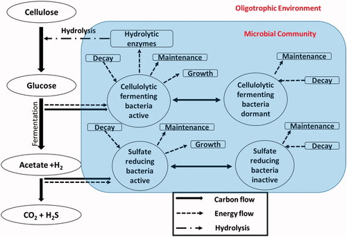
To illustrate the model dynamics, we consider a community consisting of two inter-dependent functional groups: cellulolytic fermenting bacteria (CFB) and strictly anaerobic sulfate-reducing bacteria (SRB) (Figure 1). The latter is representative of respiratory microorganisms (e.g., Desulfobacter sp.) that become active when more powerful terminal electron acceptors (TEAs), such as oxygen and nitrate, have been exhausted (Ingvorsen et al. 1984). As a general modeling framework, the catabolic energy optimization approach developed in this paper can be extended to more complex, energy-limited microbial communities by incorporating additional functional microbial groups, representing competitive interactions and substrate preferences (Amenabar et al. 2017; Zhuang et al. 2011), and by taking into account additional limiting factors, such as a lack of essential nutrients, transport rates, physical limits on habitable space, or inhibition by toxic compounds (Allison 2005; Belli et al. 2015; German et al. 2012; Kim and Fogler 2000).

Figure 1. Consortium of cellulolytic fermenting microorganisms and sulfate-reducing bacteria carrying out the complete degradation of cellulose under anaerobic conditions.

Model overview and governing equations

In natural environments, microbial communities comprise both active and dormant cells (Stolpovsky et al. 2011). The fraction of dormant microbial biomass in the subsurface typically varies between 20 and 80%, with several studies showing up to 95% of soil microorganisms being in the inactive state (Jones and Lennon 2010; Lennon and Jones 2011). Only active microorganisms are capable of growth, while only a subset of the active cells synthesizes and release exoenzymes that hydrolyze macromolecular HOM into monomers (Wilson 2011). The monomers in turn can be taken up and used as electron donors by microbial cells to generate energy. Hydrolysis of HOM is usually considered as a primary rate-controlling step in the degradation of complex natural organic matter (Eastman and Ferguson 1981; Tiehm et al. 1997; Van Cappellen and Gaillard 1996).

Hydrolysis

The model concept is illustrated in Figure 1. For simplicity, we consider a subsurface environment where the bioaccessible HOM concentration remains constant over time. That is, we implicitly assume that the in-situ consumption of HOM is balanced by the input of new HOM, for example via litter input to soil. Note that this condition can be removed by introducing a separate conservation equation for HOM to account for the temporal variations in HOM availability. The hydrolytic enzymes (HE) that break down the macromolecular compounds into monomers can be free-floating or attached to the external cell surface (Wilson 2008). We assume that the binding of the hydrolytic enzymes to HOM follows a Langmuir isotherm. If, in addition, we assume that the hydrolysis rate scales linearly with the concentration of the enzyme-HOM complexes (Vavilin et al. 2008), then the extracellular hydrolysis rate $r_{\mathit{hyd}}$ [C-mol HOM L⁻¹ d⁻¹] (carbon-mole HOM, per liter pore water, per day) can be expressed by the classical Michaelis-Menten rate law: (1) $$r_{\mathit{hyd}}=r_{\mathit{hyd}}^{\mathit{max}}·\frac{\left[HE\right]}{\left[HE\right]+K_{\mathit{hyd}}}$$(1) where $r_{\mathit{hyd}}^{\mathit{max}}$ [C-mol HOM⁻¹ d⁻¹] is the maximum hydrolysis rate, $\left[HE\right]$ [C-mol HE L⁻¹] denotes the extracellular hydrolytic enzyme concentration, and $K_{\mathit{hyd}}$ [C-mol HE L⁻¹] is the half-saturation constant for HOM hydrolysis. In principle, $r_{\mathit{hyd}}^{\mathit{max}}$ could be further expressed as the product of the bioaccessible HOM concentration and a maximum specific hydrolysis rate. To limit the number of adjustable parameters, in what follows we impose a fixed value to $r_{\mathit{hyd}}^{\mathit{max}}$ instead (see section Parameter values for details). Further note that we assume a homogenous porous medium so that the porosity does not explicitly appear in the mass conservation equations.

Energy production

Monomers produced by extracellular hydrolysis (e.g., glucose) and fermentation products (e.g., acetate and H₂) are used by active cells as direct substrates in energy-yielding (catabolic) reactions. Organic monomer concentrations are typically low (i.e., <100 µM) in natural subsurface environments, which imposes both kinetic (as embodied by the Michealis-Menten rate law) and energetic limitations on microbial activity (Jin and Bethke 2007; LaRowe et al. 2012). Cells will only carry out a given catabolic reaction when it is thermodynamically favorable. Therefore, in the rate equations describing the consumption of direct energy substrates ($r_{\mathit{des}}$) by fermentation or respiration, we explicitly include a thermodynamic function (i.e., $\max \left(0,1-\frac{\left[Q\right]}{K_{eq}}\right)$) which ranges from 0 to 1. (2) $$r_{\mathit{des}}={\mu }_{\mathit{des}}^{\mathit{max}}·X_{ac}·\frac{\left[S\right]}{\left[S\right]+K_S}·\max \left(0,1-\frac{\left[Q\right]}{K_{eq}}\right)$$(2) where ${\mu }_{\mathit{des}}^{\mathit{max}}$ is the maximum specific rate of the given catabolic reaction, $X_{ac}$ is the active biomass concentration carrying out the reaction [C-mol biomass L⁻¹], [S] is the direct energy substrate concentration and $K_S$ the corresponding half-saturation constant, and Q and K_eq are respectively, the reaction quotient and equilibrium constant of the catabolic reaction.

According to Equation 2(2) $$r_{\mathit{des}}={\mu }_{\mathit{des}}^{\mathit{max}}·X_{ac}·\frac{\left[S\right]}{\left[S\right]+K_S}·\max \left(0,1-\frac{\left[Q\right]}{K_{eq}}\right)$$(2) , the max function on the right-hand side of Equation 2(2) $$r_{\mathit{des}}={\mu }_{\mathit{des}}^{\mathit{max}}·X_{ac}·\frac{\left[S\right]}{\left[S\right]+K_S}·\max \left(0,1-\frac{\left[Q\right]}{K_{eq}}\right)$$(2) returns the largest of the numbers in parentheses. The consumption of direct energy substrates (the forward reaction) generates energy for the active cells when Q < K_eq and, therefore, 1 − Q/K_eq is a number comprised between 0 and 1. When Q > K_eq, the fermentation or respiration reaction is not thermodynamically favorable and 1 − Q/K_eq is a negative number. The max function then returns a zero value and r_des equals zero. For example, when acetate is the electron donor (ED) used by SRB, $r_{\mathit{des}}$ and ${\mu }_{\mathit{des}}^{\mathit{max}}$ are expressed in [C-mol acetate L⁻¹ d⁻¹] and [C-mol acetate C-mol biomass⁻¹ d⁻¹], respectively, and [S] and $K_S$ are both in units of [C-mol acetate L⁻¹]. Note that other formulations of the thermodynamic limitation term have been proposed in the literature, including expressions that incorporate minimum energetic thresholds, such as minimum energy required to produce ATP or to maintain a viable membrane potential (Jin and Bethke 2005, 2007; LaRowe et al. 2012).

Energy balance of active cells

In the proposed model framework, energy extracted from the direct energy substrates is used for cellular maintenance, the production of hydrolytic enzymes, and biomass growth (Figure 1). If the availability of external monomers becomes too low, cellular compounds can serve as additional energy substrates. For simplicity, we combine cell death with the utilization of non-essential energy resources from within the cell (i.e., endogenous respiration) into a single rate parameter to account for biomass decay. The energy balance of the active biomass then becomes: (3) $${-r}_{\mathit{des}}·{\Delta G}_{\mathit{des}}=r_{{ME}_{ac}}·X_{ac}+r_{HE}·{\Delta G}_{HE}+r_{gr}·{\Delta G}_{gr}+r_{\mathit{dec}}^{ac}·{\Delta G}_{\mathit{dec}}^{ac}$$(3) where $\Delta G_{\mathit{des}}<0$ is the Gibbs energy released by fermentation or respiration, $r_{{ME}_{ac}}$ > 0 [kJ/C-mol biomass L⁻¹ d⁻¹] denotes the maintenance energy utilization rate by active cells, ${\Delta G}_{HE}$ > 0 [kJ C-mol HE⁻¹] is the Gibbs energy used to produce hydrolytic enzymes, ${\Delta G}_{gr}$> 0 [kJ C-mol biomass⁻¹] is the Gibbs energy of biomass synthesis, $\Delta G_{\mathit{dec}}^{ac}<0$ [kJ C-mol biomass⁻¹] denotes the Gibbs energy released from the oxidation of cellular components, $r_{gr}$ [C-mol biomass L⁻¹ d⁻¹] is the biomass growth rate, $r_{HE}$ [C-mol HE L⁻¹ d⁻¹] is the rate of production of hydrolytic enzymes, and $r_{\mathit{dec}}^{ac}$ [C-mol biomass L⁻¹ d⁻¹] is the decay rate of the active biomass.

Gibbs energies of reaction are adjusted for changes in temperature and chemical composition using: (4) $$\Delta G_r=\Delta G_r^0+\mathit{RT}\ln Q$$(4) where $\mathrm{\Delta }{G}_{r\mathrm{ }}$ and $\Delta G_r^0$ [kJ mol⁻¹] are the actual and standard state Gibbs energies of reaction, respectively; T [K] is the absolute temperature, R = 8.314 JK⁻¹mol⁻¹ the universal gas constant, and Q the reaction quotient. The standard Gibbs energies are calculated at the specified temperature. In addition, the Gibbs energies of reaction $\Delta G_{r\mathrm{ }}$ are updated at every time step to account for the changes in the concentrations of the reactants and products.

In the model simulations, the specific maintenance energy demand ($r_{{ME}_{ac}}$) for a given microbial group is kept constant. In addition, we assume that, when allocating catabolic energy, cells give priority to fulfilling their maintenance requirements before investing in the growth or production of hydrolytic enzymes. If the catabolic energy production is insufficient to maintain the entire active biomass, there is neither cell growth nor the production of hydrolytic enzymes. Furthermore, biomass decay (cell death plus endogenous respiration) is assumed to make up for the energy shortage or, mathematically: $$\mathrm{IF}\mathrm{ }\hspace{1em}\hspace{1em}{-r}_{\mathit{des}}·{\Delta G}_{\mathit{des}}<X_{ac}·r_{{ME}_{ac}}$$ $$\mathrm{THEN}\hspace{1em}\hspace{1em}{r}_{HE}=0;\mathrm{ }{\mathrm{ }r}_{gr\mathrm{ }}=0$$ (5) $$\mathrm{AND}\hspace{1em}\hspace{1em}{r}_{\mathit{dec}}^{ac}=\mathrm{ }\frac{-r_{\mathit{des}}{·\Delta G}_{\mathit{des}}-X_{ac}{·\mathit{rME}}_{ac}}{{\Delta G}_{\mathit{dec}}^{ac}}$$(5)

Conversely, if the catabolic energy supply is larger than the maintenance requirement of the active cell population, excess energy is available for biomass growth and the production of hydrolytic enzymes.

The release of exoenzymes, including hydrolytic ones, has been shown to respond to changes in environmental conditions, such as temperature, pH, moisture content, and dissolved oxygen concentration (Hall et al. 2014; Sinsabaugh and Follstad Shah 2012; Sinsabaugh et al. 2008). Microorganisms also adjust the production of exoenzymes to the availability of the targeted external resources, although the underlying mechanisms remain poorly understood (Lynd et al. 2002; Moorhead et al. 2013; Sinsabaugh and Follstad Shah 2012). Overall, we expect the biomass-HE-HOM system to strive for a balance between maximizing access to the external resource and minimizing the wasting of exoenzymes (Wang et al. 2013). Hence, when for a given availability of HOM the HE concentration is too low, more excess catabolic energy production is diverted into the production of the enzymes. When the concentration of HE is too high, hydrolytic-enzyme production is reduced and more of the excess energy is directed toward biomass growth. Mathematically, this behavior is captured by introducing an inhibition coefficient, $K_{HE}$ [C-mol HE L⁻¹] that regulates HE production. Together with the assumption that in case of excess catabolic energy production there is no (net) biomass decay, we obtain: $$\mathrm{IF}\hspace{1em}\hspace{1em}{-r}_{\mathit{des}}{·\Delta G}_{\mathit{des}}>X_{ac}·r_{{ME}_{ac}}$$ $$\mathrm{THEN}\hspace{1em}\hspace{1em}{r}_{\mathit{dec}}^{ac}=0$$ (6) $$\mathrm{AND}\hspace{1em}\hspace{1em}\frac{r_{HE}{·\Delta G}_{HE}}{r_{HE}\mathrm{ }{·\Delta G}_{HE}+\mathrm{ }{r}_{gr}\mathrm{ }{·\Delta G}_{gr}}=\mathrm{ }\frac{K_{HE}}{\left[HE\right]+K_{HE}}$$(6) (7) $$\mathrm{AND}\hspace{1em}\hspace{1em}{r}_{gr\mathrm{ }}=\mathrm{ }\frac{{-r}_{\mathit{des}}{·\Delta G}_{\mathit{des}}-\mathrm{ }{X}_{ac}·r_{{ME}_{ac}}\mathrm{ }}{{\Delta G}_{gr}}·\frac{\left[H\mathrm{E}\right]}{\left[HE\right]+K_{HE}}$$(7) (8) $$\mathrm{AND}\hspace{1em}\hspace{1em}{r}_{HE}=\mathrm{ }\frac{-r_{\mathit{des}}{·\Delta G}_{\mathit{des}}-\mathrm{ }{X}_{ac}·r_{{ME}_{ac}}\mathrm{ }}{{\Delta G}_{HE}}·\frac{K_{HE}}{\left[HE\right]+K_{HE}}$$(8) where the inhibition function $\frac{K_{HE}}{\left[HE\right]+K_{HE}}$ varies between 0 and 1, depending on the HE concentration.

Organic monomers are not only used in energy-yielding reactions, but also in building new biomass and producing HE. For organic monomers, the net rate of consumption is therefore given by: (9) $$\frac{d\left[S\right]}{dt}=\mathrm{ }{r}_{\mathit{hyd}}-r_{\mathit{des}}-\mathrm{ }{r}_{C_{gr}}-r_{C_{HE}},$$(9) where $r_{C_{gr}}$ and $r_{C_{HE}}$ [C-mol L⁻¹ d⁻¹] are the rates of organic monomer utilization for growth and HE production, respectively.

Dormancy

An important strategy for microorganisms to survive under unfavorable conditions is to switch to a dormant state (Stolpovsky et al. 2011). Dormancy creates a microbial seed bank ready to be resuscitated upon the return of more favorable conditions (Lennon and Jones 2011). In our model, the switching between active and dormant states is controlled by the relative magnitudes of the catabolic energy production and the maintenance requirement of a given microbial functional group: when the maintenance energy rate is greater than the catabolic energy production, active cells enter the dormant state. In the opposite case, dormant cells resuscitate. As shown by Stolpovsky et al. (2011), this behavior can be captured by using a dimensionless switch function, $\theta ,$ that regulates the activation and deactivation rates. Stolpovsky et al. (2011) formulated $\theta$ based on Fermi-Dirac statistics. Here, we present the following alternative formulation: (10) $$\theta =0.5\mathrm{ }·\left[\tanh \left(\frac{{-r}_{\mathit{des}}·{\Delta G}_{\mathit{des}}}{X_{ac}·r_{{ME}_{ac}}}-1\right)+1\right],$$(10) with $\theta$-values ranging between 0 and 1. The switch function presented in Equation 10(10) $$\theta =0.5\mathrm{ }·\left[\tanh \left(\frac{{-r}_{\mathit{des}}·{\Delta G}_{\mathit{des}}}{X_{ac}·r_{{ME}_{ac}}}-1\right)+1\right],$$(10) produces similar results as the equation proposed by Stolpovsky et al. (2011). These authors analyzed data from laboratory experiments in which microorganisms were exposed to a discontinuous supply of substrate and reactivated after variable periods of starvation. Equation 1(1) $$r_{\mathit{hyd}}=r_{\mathit{hyd}}^{\mathit{max}}·\frac{\left[HE\right]}{\left[HE\right]+K_{\mathit{hyd}}}$$(1) yields an equally good fit to the same dataset (results not shown).

The deactivation rate $r_{\mathit{deac}}$ [C-mol biomass L⁻¹d⁻¹] is then calculated as: (11) $$r_{\mathit{deac}}=k_{\mathit{deac}}·\left(1-\theta \right)·X_{ac},$$(11) in which $k_{\mathit{deac}}$ [d⁻¹] is the deactivation rate coefficient. The activation rate $r_{ac}$ [C-mol biomass⁻¹ L⁻¹ d⁻¹] is obtained from: (12) $$r_{ac}=k_{ac}·\theta ·X_{in},$$(12) where $k_{ac}$ [d⁻¹] is the activation rate coefficient and $X_{in}$ [C-mol biomass L⁻¹] is the concentration of the inactive biomass.

Equation 10(10) $$\theta =0.5\mathrm{ }·\left[\tanh \left(\frac{{-r}_{\mathit{des}}·{\Delta G}_{\mathit{des}}}{X_{ac}·r_{{ME}_{ac}}}-1\right)+1\right],$$(10) yields θ-values approaching zero when the catabolic energy production ($-r_{\mathit{des}}·\Delta G_{\mathit{des}}$) is small compared to the maintenance energy requirement of the active microbial population ($X_{ac}·r_{{ME}_{ac}}$). In contrast, when the catabolic energy gain largely exceeds the maintenance requirement, θ is close to one, and inactive cells transform into active cells. The use of the switch function (θ) to simulate the dynamic response of the partitioning between active and dormant cells is similar to that proposed by Stolpovsky et al. (2011), who analyzed data from laboratory experiments in which microorganisms were exposed to a discontinuous supply of substrate and reactivated after variable periods of starvation.

Energy balance of dormant cells

The dormant microorganisms are assumed to be unable to use external substrates to grow or produce HE. However, they still need to invest some energy to maintain their molecular and cellular integrity, albeit at much lower rates than active cells. Dormant cells can use endogenous compounds, such as glycogen or hydroxyalkanoates, as energy substrates, resulting in a reduction of biomass (Lennon and Jones 2011). The corresponding energy balance can be written as: (13) $$X_{in}·r_{{ME}_{in}}+r_{\mathit{dec}}^{in}·\Delta G_{\mathit{dec}}^{in}=0$$(13) resulting in: (14) $$r_{\mathit{dec}}^{in}=\mathrm{ }\frac{X_{in}·r_{{ME}_{in}}}{{-\Delta G}_{\mathit{dec}}^{in}}$$(14) where $r_{{ME}_{in}}$ [kJ C-mol biomass⁻¹d⁻¹] is the maintenance energy requirement of the inactive biomass, ${\Delta G}_{\mathit{dec}}^{in}$ [kJ C-mol biomass⁻¹] is the Gibbs energy gained from the degradation of cellular constituents, and $r_{\mathit{dec}}^{in}$ is the decay rate of inactive biomass [C-mol biomass L⁻¹d⁻¹]. Note that, as for the active cells, we use the term decay to include all processes leading to a reduction in the microbial biomass, that is, endogenous respiration and cell lysis.

Conservation equations for biomass and hydrolytic enzymes

The conservation equations for the microbial biomasses of the active and inactive cells, X_ac and X_in, and the concentration of HE are: (15) $$\frac{{dX}_{ac}}{dt}=r_{gr}+r_{ac}-r_{\mathit{deac}}-r_{\mathit{dec}}^{ac}$$(15) (16) $$\frac{{dX}_{in}}{dt}=r_{\mathit{deac}}-r_{ac}-r_{\mathit{dec}}^{in}$$(16) (17) $$\frac{d\left[HE\right]}{dt}=\mathrm{ }{r}_{HE}-\mathrm{ }{k}_{\mathit{dec}}^{HE}·\left[HE\right]$$(17) where $k_{\mathit{dec}}^{HE}$ [d⁻¹] is the first-order HE decay rate coefficient. Spatial distributions of the biomasses can, in principle, be computed by coupling Equations 15–17 to transport calculations, while the response to temporal changes in bioaccessible HOM could be simulated by adding a conservation equation that accounts for the external and internal sources and sinks of HOM in the subsurface system of interest.

Application: Anaerobic cellulose degradation

Reaction system

Cellulose is a major constituent of terrestrial plant detritus (Béguin and Aubert 1994; Leschine 1995; Lynd et al. 2002; Pérez et al. 2002). It is used here as a representative of HOM in continental subsurface environments. Microorganisms use a variety of hydrolytic enzymes to degrade cellulose via several different pathways, which have yet to be completely characterized (Wilson 2009, 2011). In anaerobic environments, cellulolytic fermentative microorganisms can obtain energy for growth from cellulose degradation (Jurtshuk 1996). Fermentation of glucose, resulting from cellulose hydrolysis, produces CO₂, H₂, and different combinations of intermediate products, such as ethanol, formate, acetate, lactate, and succinate (Christensen et al. 2000; Leschine 1995; Lovley and Chapelle 1995). These fermentation products may serve as electron donors to other anaerobic microorganisms. Microbial communities that include cellulolytic fermenters operating in concert with heterotrophic microorganisms can therefore completely oxidize cellulose to CO₂.

The microbial community considered here consists of two interacting microbial functional groups: cellulolytic fermenting bacteria (CFB) and sulfate-reducing bacteria (SRB). We assume that only the fermenters can hydrolyze cellulose, while the sulfate reducers depend on the metabolites produced by fermenters as their energy source (Wilson 2008; Wrighton et al. 2014). Under strictly anaerobic conditions, synergistic communities of CFB and SRB are known to completely degrade cellulose to carbon dioxide with the production of sulfide (Leschine 1995). Both SRB and sulfate are commonly found in suboxic and anoxic soils and sediments. However, the proposed modeling approach can be extended to microbial groups using terminal electron acceptors (TEAs) other than sulfate, for example, ferric iron mineral phases or organic electron acceptors.

The CFB performs two key tasks in the model: (1) extracellular cellulolytic enzyme production for the hydrolysis of cellulose to glucose, and (2) glucose fermentation (Figure 1). We assume that glucose fermentation produces acetate (CH3COO–) and H₂, intermediates commonly observed during the anaerobic degradation of natural organic matter (Novelli et al. 1988). Acetate is considered one of the main carbon and energy substrates fueling respiration in anaerobic sediments (Roden 2008). Many organic compounds, such as ethanol, lactate, propionate, and butyrate, produced as by-products of fermentation processes usually transform into acetate and H₂ before complete oxidation to CO₂ (Leschine 1995; Lovley and Chapelle 1995). Hence, the following simplified reaction is used to represent glucose fermentation: (18) $${\mathrm{C}}_6{\mathrm{H}}_{12}{\mathrm{O}}_6+{4\mathrm{H}}_2\mathrm{O}\mathrm{\to }{2\mathrm{C}\mathrm{H}}_3{\mathrm{COO}}_{-}+{2\mathrm{H}\mathrm{CO}}_{3-}+{4\mathrm{H}}^{+}+{4\mathrm{H}}_{2\left(\mathrm{aq}\right)}$$(18)

Natural populations of SRB utilize H₂ and a variety of small organic compounds as energy substrates (Plugge et al. 2011). In the model, the latter are collectively represented by acetate. The corresponding sulfate-reducing pathways are then: (19) $${\mathrm{CH}}_3{\mathrm{COO}}^{-}+{{\mathrm{SO}}_4}^{2-}\mathrm{\to }{2\mathrm{H}\mathrm{CO}}_{3-}+{\mathrm{HS}}^{-},$$(19) (20) $${4\mathrm{H}}_{2\left(\mathrm{aq}\right)}+{\mathrm{H}}^{+}+{{\mathrm{SO}}_4}^{2-}\mathrm{\to }{\mathrm{HS}}^{-}+{4\mathrm{H}}_2\mathrm{O}.$$(20)

The rates of sulfate reduction by these two pathways are calculated by Equation 2(2) $$r_{\mathit{des}}={\mu }_{\mathit{des}}^{\mathit{max}}·X_{ac}·\frac{\left[S\right]}{\left[S\right]+K_S}·\max \left(0,1-\frac{\left[Q\right]}{K_{eq}}\right)$$(2) and, thus, these rates depend on the concentrations of the reactants and products in Equations 19(19) $${\mathrm{CH}}_3{\mathrm{COO}}^{-}+{{\mathrm{SO}}_4}^{2-}\mathrm{\to }{2\mathrm{H}\mathrm{CO}}_{3-}+{\mathrm{HS}}^{-},$$(19) and 20(20) $${4\mathrm{H}}_{2\left(\mathrm{aq}\right)}+{\mathrm{H}}^{+}+{{\mathrm{SO}}_4}^{2-}\mathrm{\to }{\mathrm{HS}}^{-}+{4\mathrm{H}}_2\mathrm{O}.$$(20) via the corresponding reaction quotients. Sulfide, produced by the reduction of sulfate, is assumed to react rapidly with ferric iron-containing mineral phases to form insoluble ferrous iron sulfides (Rickard and Luther 1997), hence avoiding the accumulation of free sulfide to toxic levels (Reis et al. 1992). Similarly, we assume that H₂ concentrations remain low and constant because H₂ produced by fermentation is transferred directly to the H₂ consuming SRB (Novelli et al. 1988). Consequently, H₂S and H₂ losses to the gas phase are considered to be negligible. It is important to note that by consuming H₂ (Equation 20(20) $${4\mathrm{H}}_{2\left(\mathrm{aq}\right)}+{\mathrm{H}}^{+}+{{\mathrm{SO}}_4}^{2-}\mathrm{\to }{\mathrm{HS}}^{-}+{4\mathrm{H}}_2\mathrm{O}.$$(20) ) and acetate (Equation 19(19) $${\mathrm{CH}}_3{\mathrm{COO}}^{-}+{{\mathrm{SO}}_4}^{2-}\mathrm{\to }{2\mathrm{H}\mathrm{CO}}_{3-}+{\mathrm{HS}}^{-},$$(19) ), the SRB help maintains thermodynamically favorable conditions for the CFB. Further note that, in the model, the SRB does not produce HE. Thus, any catabolic energy produced by the SRB in excess of their maintenance energy requirement is invested in new biomass growth.

According to the stoichiometry of the glucose-fermentation reaction (Equation 18(18) $${\mathrm{C}}_6{\mathrm{H}}_{12}{\mathrm{O}}_6+{4\mathrm{H}}_2\mathrm{O}\mathrm{\to }{2\mathrm{C}\mathrm{H}}_3{\mathrm{COO}}_{-}+{2\mathrm{H}\mathrm{CO}}_{3-}+{4\mathrm{H}}^{+}+{4\mathrm{H}}_{2\left(\mathrm{aq}\right)}$$(18) ), 2/3 of the carbon from glucose goes to acetate and 1/3 to bicarbonate, while 2/3 moles of H₂ are formed per mole glucose carbon consumed. The conservation equations for acetate and H₂ are then given by: (21) $$\frac{\mathrm{d}\left[Ac\right]}{\mathrm{d}t}=\frac{2}{3}{r}_{\mathit{ferm}}-r_{Ac}-r_{C_{gr,\mathit{SRB}}}$$(21) and (22) $$\frac{\mathrm{d}\left[H_2\right]}{\mathrm{d}t}=\frac{2}{3}{r}_{\mathit{ferm}}-r_{H_2}$$(22) where $\left[Ac\right]$ [C-mol L⁻¹] and ${[H}_2]\mathrm{ }$[mol H₂ L⁻¹] are the concentrations of acetate and H₂, $r_{\mathit{ferm}\mathrm{ }}$ [C-mol L⁻¹d⁻¹] is the rate of fermentation, which replaces the generic direct energy substrate consumption rate $r_{\mathit{des}\mathrm{ }}$ in Equation 2(2) $$r_{\mathit{des}}={\mu }_{\mathit{des}}^{\mathit{max}}·X_{ac}·\frac{\left[S\right]}{\left[S\right]+K_S}·\max \left(0,1-\frac{\left[Q\right]}{K_{eq}}\right)$$(2) , and $r_{Ac}$ [C-mol L⁻¹d⁻¹] and $r_{H_2}$ [mol H₂ L⁻¹ d⁻¹] are the rates of acetate and H₂ consumption by SRB, respectively, and $r_{C_{gr,\mathit{SRB}}}$ [C-mol L⁻¹d⁻¹] is the rate of acetate additionally consumed when serving as a carbon source for biomass synthesis by (active) SRB.

Parameter values

The default parameter values used in the simulations are listed in Table 1. They are representative of natural aquifers and water-logged soils although the ranges of most parameters can be quite large. A determining parameter controlling the organic matter degradation and associated microbial dynamics is the maximum cellulose hydrolysis rate $(r_{\mathit{hyd}}^{\mathit{max}}).$ Previous studies report highly variable hydrolysis rates of HOM depending on, among others, the organic matter source, soil structure and texture, mineral content, microbial community structure, and the type of hydrolytic enzymes (Bezerra and Dias 2004; Small et al. 2008). Observed specific rates of HOM hydrolysis vary between 0.2 and 0.00002 d⁻¹ (Roden 2008; Roden and Wetzel 2002; Rotter et al. 2008). The baseline $r_{\mathit{hyd}}^{\mathit{max}}\mathrm{ }$ value used here is an average estimated from reported carbon turnover rates in soils and sediments (Canfield et al. 2005; Roden 2008; Roden and Wetzel 2002; Rotter et al. 2008). The value of the half-saturation constant of cellulose hydrolysis (K_hyd = 10⁻⁵ C-mol POM L⁻¹) is an educated guess. As Resat et al. (2012) showed in their cellulose degradation simulations, the overall model outcomes are relatively insensitive to the chosen value of K_hyd, unless extreme values are chosen. The same applies to the simulations performed here for variable K_hyd values (results not shown).

Table 1. Default parameter values.

Parameter	Description	Value	Units	References
$r_{\mathit{hyd}}^{\mathit{max}}$	Maximum hydrolysis rate	1.1 × 10^−5	[C-mol POM L^−1 d^−1]	Calculated based on Roden and Wetzel 2002; Canfield et al. 2005; Roden 2008; Rotter et al. 2008
$r_{Ac}^{\mathit{max}}$	Maximum specific acetate utilization rate by sulfate-reducing bacteria	29.3	[d^−1]	Calculated based on Scheibe et al. (2009)
$r_{H2}^{\mathit{max}}$	Maximum specific hydrogen utilization rate by sulfate-reducing bacteria	7.7	[d^−1]	Khosrovi et al. 1971
$r_{\mathit{ferm}}^{\mathit{max}}$	Maximum specific fermentation rate	5.4	[d^−1]	Calculated based on Scheibe et al. (2009)
${\mathit{rME}}_{ac, \mathit{SRB}}$	Maintenance-energy requirement for active sulfate-reducing bacteria	17.8	[kJ C-mol biomass^−1 d^−1]	Tijhuis et al. 1993
${\mathit{rME}}_{in, \mathit{SRB}}$	Maintenance-energy requirement for inactive sulfate-reducing bacteria	0.31	[kJ C-mol biomass^−1 d^−1]	Anderson and Domsch 1985
${\mathit{rME}}_{in, \mathit{CFB}}$	Maintenance-energy requirement for inactive cellulolytic fermenters	0.31	[kJ C-mol biomass^−1 d^−1]	Anderson and Domsch 1985
${\mathit{rME}}_{ac, \mathit{CFB}}$	Maintenance-energy requirement for active cellulolytic fermenters	17.8	[kJ C-mol biomass^−1 d^−1]	Tijhuis et al. 1993
${\Delta G}_{gr, \mathit{SRB}}$	Gibbs energy required for biomass growth of sulfate reducing bacteria	426	[kJ C-mol biomass^−1 d^−1]	Empirical formula of Heijnen and Dijken (1992) with acetate as the C-source
${\Delta G}_{\mathit{dec}, \mathit{CFB}}^{ac}$	Gibbs energy gained from decaying biomass of active cellulolytic fermenters	67	[kJ C-mol biomass^−1 d^−1]	Heijnen and Dijken 1992
${\Delta G}_{\mathit{dec}, \mathit{CFB}}^{in}$	Gibbs energy gained from decaying biomass of dormant fermenters	67	[kJ C-mol biomass^−1 d^−1]	Heijnen and Dijken 1992
${\Delta G}_{\mathit{dec}, \mathit{SRB}}^{in}$	Gibbs energy gained from decaying biomass of dormant sulfate-reducing bacteria	67	[kJ C-mol biomass^−1]	Heijnen and Dijken 1992
${\Delta G}_{\mathit{dec}, \mathit{SRB}}^{ac}$	Gibbs energy gained from decaying biomass of active sulfate-reducing bacteria	67	[kJ C-mol biomass^−1]	Heijnen and Dijken 1992
${\Delta G}_{gr, \mathit{CFB}}$	Gibbs energy required for biomass growth of fermenting bacteria	211	[kJ C-mol biomass^−1]	Empirical formula of Heijnen and Dijken (1992) with glucose as the C-source
${\Delta G}_{HE}$	Gibbs energy required to produce hydrolytic enzymes	2.93	[kJ C-mol HE^−1]	Zhang and Lynd 2005
$k_{\mathit{dec}}^{HE}$	Decay rate coefficient of hydrolytic enzymes	0.005	[d^−1]	Calculated based on Resat et al. (2012)
$K_{HE}$	Half-saturation/inhibition constant regulating the concentration of hydrolytic enzymes	1 × 10^−5	[C-mol HE L^−1]	Back calculated
$K_{Ac}$	Half-saturation constant for acetate in sulfate reduction	2 × 10^−3	[C-mol ED L^−1]	Roden 2008 and reference there within
$K_H$	Half-saturation constant for H2 in sulfate reduction	1 × 10^−5	[mol H2 L^−1]	Dale et al. 2006
$K_S$	Half-saturation constant for glucose in fermentation	1.33 × 10^−4	[C-mol ED L^−1]	Kleman and Strohl 1994
$k_{\mathit{deac}, \mathit{CFB}}$	Deactivation rate coefficient of fermenters	1.2	[d^−1]	Stolpovsky et al. 2011
$k_{\mathit{deac}, \mathit{SRB}}$	Deactivation rate coefficient of sulfate-reducing bacteria	1.2	[d^−1]	Stolpovsky et al. 2011
$k_{\mathit{act}, \mathit{CFB}}$	Activation rate coefficient of fermenters	1.2	[d^−1]	Stolpovsky et al. 2011
$k_{\mathit{act}, \mathit{SRB}}$	Activation rate coefficient of sulfate-reducing bacteria	1.2	[d^−1]	Stolpovsky et al. 2011

The maintenance energy requirements for active bacteria ($r_{{ME}_{ac}}$) and the Gibbs energies for biomass growth (${\Delta G}_{gr}$) for different microbial groups are also major parameters in the model because they control the distribution of the catabolic energy among the different cellular functions (see section Sensitivity analysis). The value of $r_{{ME}_{ac}}$ determines the catabolic energy production threshold that needs to be exceeded to enable biomass growth. The maintenance energy requirements of microorganisms and their dependence on environmental conditions remain poorly known (Hoehler 2004). For the active SRB and CFB, we use the temperature-dependent empirical expression for anaerobic microorganisms proposed by Tijhuis et al. (1993) at a groundwater temperature of 10 °C. The dormant bacteria are assigned the $r_{{ME}_{ac}}$ value derived from experiments with agricultural soil (Anderson and Domsch 1985). The Gibbs energies for biomass synthesis, ${\Delta G}_{gr},$ of the microorganisms are calculated by the empirical expression of Heijnen and Dijken (1992), with glucose and acetate as the carbon sources for CFB and SRB, respectively. Microbial biomass composition is variable, even for the same species (Popovic 2019). Here, we adopt the general biomass formula of C₅H₉O_2.5N proposed by Roels (1980), with the equivalent C-mol biomass formula of CH_1.8O_0.5N_0.2 and corresponding molecular weight of 24.6 g per C-mol biomass and cell weight of 10⁻¹³ gcell⁻¹.

The chemical concentrations and microbial biomasses imposed as initial conditions in the simulations are listed in Table 2. They are based on literature values for natural aquifers of the concentrations of hydrogen sulfide (Detmers et al. 2001), sulfate (Lovley and Chapelle 1995), and acetate, glucose plus dihydrogen (Lovley and Chapelle 1995; Lovley and Phillips 1989; Novelli et al. 1988). Unless otherwise specified, the catabolic Gibbs energies of reaction are updated at each time step according to Equation 4(4) $$\Delta G_r=\Delta G_r^0+\mathit{RT}\ln Q$$(4) to account for changes in the concentrations of reactants and products in the various metabolic processes. Temperature is held constant at 10 °C. We further assume that the reaction Gibbs energies for the decay of dormant and active biomasses are identical and that the same activation and deactivation rate coefficients apply to both CFB and SRB. The system of ordinary differential equations describing the time-dependent changes in chemical and microbial concentrations are solved with the MATLAB solver ode15s (Shampine and Reichelt 1997).

Table 2. Initial concentration used in the simulation.

Description	Value	Units
Acetate concentration	1 × 10^−5	[C-mol L^−1]
Glucose concentration	1 × 10^−7	[C-mol L^−1]
Dihydrogen concentration	1 × 10^−9	[C-mol biomass L^−1]
Active cellulolytic fermenting bacteria	1 × 10^−6	[C-mol biomass L^−1]
Dormant cellulolytic fermenting bacteria	1 × 10^−6	[C-mol biomass L^−1]
Active sulfate reducing bacteria	1 × 10^−6	[C-mol biomass L^−1]
Dormant sulfate reducering bacteria	1 × 10^−6	[C-mol biomass L^−1]
Temperature	283.15	[K]
Biochemical standard Gibbs energy for sulfate respiration with dihydrogen	−55.82	[kJ mol^−1]
Biochemical standard Gibbs energy for sulfate respiration with acetate	−47.83	[kJ C-mol^−1]
Biochemical standard Gibbs energy for glucose fermentation into acetate and dihydrogen	−135.93	[kJ C-mol^−1]
Biochemical standard state Gibbs energy for sulfate respiration with dihydrogen at 10 °C	−56.06	[kJ mol^−1]
Biochemical standard state Gibbs energy for sulfate respiration with acetate at 10 °C	−48.86	[kJ C-mol^−1]
Biochemical standard state Gibbs energy for glucose fermentation into acetate and dihydrogen at 10 °C	−190.94	[kJ C-mol^−1]
Standard Gibbs energy for sulfate respiration with dihydrogen	−75.59	[kJ mol^−1]
Standard Gibbs energy for sulfate respiration with acetate	−87.77	[kJ C-mol^−1]
Standard Gibbs energy for glucose fermentation into acetate and dihydrogen	23.8	[kJ C-mol^−1]
Standard state Gibbs energy for sulfate respiration with dihydrogen at 10 °C	−75.02	[kJ mol^−1]
Standard state Gibbs energy for sulfate respiration with acetate	−84.79	[kJ C-mol^−1]
Standard state Gibbs energy for glucose fermentation into acetate and dihydrogen at 10 °C	−39.22	[kJ C-mol^−1]
Gibbs energy for sulfate respiration with dihydrogen at the initial concentrations	−8.96	[kJ mol^−1]
Gibbs energy for sulfate respiration with acetate at the initial concentrations	−24.61	[kJ C-mol^−1]
Gibbs energy for glucose fermentation into acetate and dihydrogen at the initial concentrations	−68.97	[kJ C-mol^−1]
Hydrogen sulfide concentration	5.73 × 10^−6	[mol L^−1]
Bicarbonate concentration	3.44 × 10^−3	[mol L^−1]
H^+ concentration	1 × 10^−7	[mol L^−1]
Sulfate concentration	4.68 × 10^−5	[mol L^−1]

Results and discussion

Model stability and response time scale

The stability of the numerical model was verified by running numerous simulations with variable initial values for the chemical and microbial concentrations (results not shown). In all cases, the simulations converged to the same steady-state as illustrated in Supplementary Figure S1 for initial total microbial biomasses ranging between 4 × 10⁻⁸ and 4 × 10⁻⁴ C-mol biomass L⁻¹, or ∼10⁴–10⁸ cells mL⁻¹. Notwithstanding the order-of-magnitude differences in initial values, the same steady-state total biomass concentration is reached. The concentrations and biomasses exhibit their most rapid changes in the first 100 days and approach their steady-state values within 300 days.

Baseline simulation: Initial (non-steady-state) phase

The baseline kinetic and bioenergetic-based parameter values (Table 1) were selected to be representative of the biogeochemical dynamics in shallow groundwater systems. As initial conditions (Table 2), we imposed relatively low concentrations of the bacterial biomasses. As expected, the largest changes in the concentrations of electron donors and hydrolytic enzymes, as well as in active and dormant biomasses, occurred during the first 100 days, with only relatively small changes beyond 300 days (Figure 2, see also Supplementary Figure S2). Note that in the baseline simulation, the sulfate concentration is kept constant at 47 µmol L⁻¹.

Figure 2. Non-steady state baseline simulation: (A) concentrations of electron-donors and hydrolytic enzymes, and (B) biomasses of active and dormant bacteria at selected time points. All concentrations are given in moles carbon per unit pore water volume, except for dihydrogen, which is in moles dihydrogen per unit pore water volume.

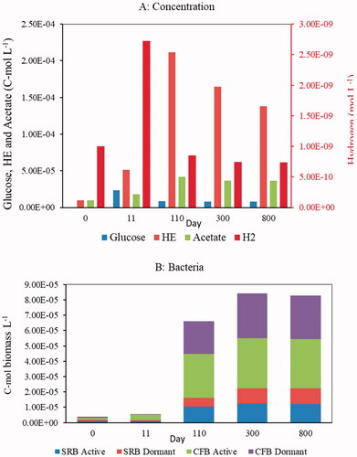
Under the initial conditions imposed in the baseline simulation, the available direct energy substrates (glucose, acetate, and dihydrogen) are insufficient to provide the two groups of bacteria with sufficient energy for growth. That is, at the beginning of the simulation, the maintenance energy requirements for both active CFB and SRB are higher than the catabolic energy generated through fermentation or sulfate reduction (Figure 3, see also Supplementary Figure S3). Consequently, the bacteria compensate for the energy gap by using endogenous reserves and the active biomasses decrease while the dormant biomasses increase (see inset of Supplementary Figure S2B). However, HOM hydrolysis quickly causes a rapid increase in the direct electron donor concentrations (Figure 2(A) and Supplementary Figure S2(A)), which in turn increases the catabolic energy production by both types of bacteria (Figure 3 and Supplementary Figure S3).

Figure 3. Non-steady state baseline simulation: (A) cellulolytic fermenting bacteria (CFB) and (B) sulfate-reducing bacteria (SRB). The panels compare (i) the total daily rates of Gibbs energy production by the cells (TE_CFB and TE_SRB), (ii) the daily rates of Gibbs energy consumption by the cells to grow new biomass (G_CFB and G_SRB), and (iii) the daily rates of Gibbs energy consumption by the CFB to produce extracellular hydrolytic enzymes (E_HE). The daily rates are expressed per unit of biomass carbon. Also shown on the panels are the specific growth rates of CFB and SRB (µ_CFB and µ_SRB). The black lines represent the specific maintenance energy requirements of the bacteria, in units of kJ per C-mol biomass per day.

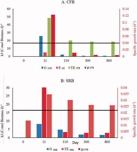
Once the energy gained from glucose fermentation exceeds the maintenance energy requirement, CFB starts growing rapidly (Supplementary Figure S3(A)). The onset of growth of the SRB lags behind that of the CFB (Supplementary Figure S3(B)) because the CFB first has to produce the direct energy substrates that can be used by the SRB (i.e., acetate and dihydrogen). The initial increases in active CFB and SRB are accompanied by decreased concentrations of the dormant bacteria in response to the favorable energetic conditions. Within two weeks, the energy gained from fermentation reaches its maximum value. At the same time, the specific growth rate of the CFB reaches its highest value of 0.12 d⁻¹. Large fractions of the catabolic energy are spent by the CFB on the production of hydrolytic enzymes and growth during this early period, which also results in high growth yields (Figure 4). The SRB follow the same pattern for growth, although the total catabolic energy production of the SRB (TE_SRB) reaches the corresponding maintenance energy requirement about 5 days later than the CFB, at which point the specific growth rate of the SRB (µ_SRB) rises sharply to a maximum value of 0.06 d⁻¹.

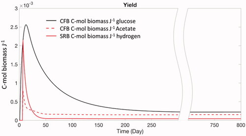
Figure 4. Non-steady state baseline simulation: growth yields in moles biomass carbon produced per unit catabolic energy biomass generated for the three different electron donors.

After about two weeks, the glucose concentration begins to decline due to the consumption by the growing CFB population, followed by declining dihydrogen and acetate concentrations. As a consequence, net growth rates of CFB and SRB decrease and, after about 300 days, the populations approach their final, steady-state, biomasses. The intricate interplay between abundance and activity of the bacteria and solute concentrations explains the early peak values of the dissolved electron donors and hydrolytic enzymes (Figure 2(A)), as well as the growth yields (Figure 4). Note that, along with the growth of the active bacterial biomasses, there are also corresponding increases in the dormant biomasses. This is because, even under energetically favorable conditions, Equation 10(10) $$\theta =0.5\mathrm{ }·\left[\tanh \left(\frac{{-r}_{\mathit{des}}·{\Delta G}_{\mathit{des}}}{X_{ac}·r_{{ME}_{ac}}}-1\right)+1\right],$$(10) predicts that a non-zero fraction of the biomass goes dormant. Hence, at a steady-state, the system comprises both active and dormant cells.

Baseline simulation: Steady-state

At steady state, the active and dormant CFB biomasses are 3.2 × 10⁻⁵ C-mol L⁻¹ (3.9 × 10⁷ cells cm⁻³) and 2.9 × 10⁻⁵ C-mol L⁻¹ (3.5 × 10⁷ cells cm⁻³), respectively. Thus, for the parameter values used here, slightly over 50% of the CFB are in the active state (Figure 2(B)). The relatively large population size of dormant cells is made possible by their much lower maintenance energy requirement compared to active cells (Table 1). In their approach to steady-state, the SRB follows a similar growth and decay pattern as the CFB, but with a slight time delay. At steady state, the active and dormant SRB biomasses are 1.2 × 10⁻⁵ C-mol biomass L⁻¹ (1.5 × 10⁷ cells cm⁻³) and 1.0 × 10⁻⁶ C-mol biomass L⁻¹ (1.2 × 10⁷ cells cm⁻³), respectively. Again, the active cells slightly exceed 50% of the total SRB population, which is not surprising given that the active and dormant SRB were assigned the same maintenance energy requirements as their CFB counterparts (Table 1).

A near-equal partitioning between active and dormant bacteria is consistent with typical percentages of dormant cells reported for both marine and freshwater environments (20–80%; Lennon and Jones 2011). The total combined active and dormant CFB and SRB biomass at steady-state is 8.3 × 10⁻⁵ C-mol biomass L⁻¹ (1.0 × 10⁸ cells cm⁻³), which is at the higher end of the range of bacterial concentrations in shallow aquifers (10⁵–10⁸ cells cm⁻³, Griebler and Lueders 2009). The model likely predicts relatively high cell concentrations because the effects of natural predators or bacteriophages are neglected, while in real aquifers these may exert a strong control on the steady-state population sizes of bacteria (Bajracharya et al. 2014).

The predicted steady-state concentrations of hydrolytic enzymes, glucose, acetate and dissolved dihydrogen are 1.4 × 10⁻⁵ C-mol HE L⁻¹, 8.0 × 10⁻⁶ C-mol L⁻¹, 3.6 × 10⁻⁵ C-mol L⁻¹, and 7.4 × 10⁻¹⁰ M, respectively (Figure 2(A)). For dihydrogen and acetate, the modeled concentrations are comparable to values reported in the literature for anoxic sediments, with concentrations of H₂ and acetate of 1–2 × 10⁻⁹mol L⁻¹ (Hoehler et al. 1998; Lovley and Goodwin 1988) and 5 × 10⁻⁵ C-mol L⁻¹ (Jin and Bethke 2009), respectively. Similarly, glucose concentrations on the order of 10⁻⁶ C-mol L⁻¹ have been observed in anaerobic and marine sediments (Lovley and Phillips 1989).

The catabolic energy production rates by active CFB and SRB at a steady-state are 18.7 and 19.4 kJ C-mol biomass⁻¹ d⁻¹, respectively, compared to the assumed maintenance energy rate of 17.8 kJ C-mol biomass⁻¹ d⁻¹ for both microbial groups. At a steady-state, the active CFB invest 95% of their catabolic energy production in maintenance, 4.6% in growth (which eventually ends up supporting maintenance in dormant cells), and the remaining in the synthesis and exudation of hydrolytic enzymes. The active SRB allocates 92% of their catabolic energy to maintenance activities and the remaining 8% to growth. These results are in line with observations for energy-limited oligotrophic environments (Del Giorgio and Cole 1998; Russell 1986) where bacterial growth efficiencies may be as low as 1% (Del Giorgio and Cole 1998). At a steady-state, the modeled specific growth rates are ∼0.004 d⁻¹ for both CFB and SRB, which corresponds to a doubling time of about half a year.

Dynamic vs. static growth yields

In many models simulating subsurface geomicrobial activity, the growth yields that relate biomass growth to substrate turnover are assumed to be constant (e.g., Scheibe et al. 2006). However, as demonstrated by Roden and Jin (2011), microbial growth yields correlate positively with the catabolic Gibbs energy production. Hence, for a given catabolic pathway the growth yield should be treated as a variable function that responds to changes in the rate at which the cells generate usable energy (e.g., Heijnen and Dijken 1992; Smeaton and Van Cappellen 2018). Our model explicitly accounts for the dynamic behavior of growth yields by calculating how the catabolic energy production rates of CFB and SRB change over time. This is illustrated in Figure 4 for the growth yields in the baseline simulation. During the early stage of the simulation, the growth yields of both CFB and SRB peak because of the rising catabolic energy production by both microbial groups. Similar early peak values are observed for the specific growth rates (Supplementary Figure S3).

In the model, the SRB utilize both acetate and molecular hydrogen as an energy source, but only acetate acts as the carbon source. Therefore, SRB growth yields for both energy substrates are shown separately in Figure 4. Only the portion of acetate that is oxidized to CO₂ to produce catabolic energy is included in the growth yield calculation. The same separation between catabolic energy generation and utilization in new biomass growth is made for the CFB, but now assuming the CFB use glucose as both their carbon and energy source. When a steady state is reached, the growth yield of CFB equals 0.22 × 10⁻³ C-mol J⁻¹. The yields of the SRB from acetate and hydrogen are 0.15 × 10⁻³ and 0.05 × 10⁻³ C-mol J⁻¹, respectively.

Although the catabolic Gibbs energy produced per unit carbon biomass is higher for the SRB than the CFB (Supplementary Figure S3), the growth yields (Figure 4) and concentrations of SRB (Figure 2) are smaller than for the CFB. The explanation lies in the energetic costs of biomass synthesis from different carbon sources. Heijnen and Dijken (1992) proposed that the more dissimilar the carbon source is from the biomass-building intermediate molecules (such as pyruvate or acetyl-CoA), with respect to the redox state and number of carbon atoms in the molecules, the more energy is dissipated because of the increased number of intermediate reaction steps. In other words, more energy (i.e., ΔG_gr) is needed to form SRB biomass from acetate than CFB biomass from glucose.

Dynamic vs. static Gibbs reaction energies

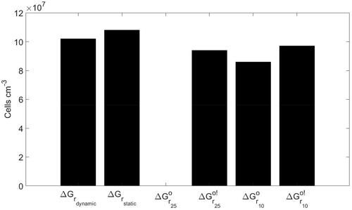
In the baseline simulation, the Gibbs reaction energies are updated at each time step to account for the changes in the reaction quotients of the energy-producing catabolic pathways (scenario 1 in Table 3). Here, the steady-state results of the baseline simulation are compared to those where the catabolic reaction energies are held constant, all other conditions unchanged (scenarios 2–6 in Table 3). The five additional scenarios are the following: in scenario 2 the Gibbs reaction energies remain the same as those calculated using the initial concentrations listed in Table 2 (${\mathrm{\Delta }G}_{r_{\mathit{static}}}$), in scenario 3 the Gibbs reaction energies are fixed to their standard values at 25 °C$\mathrm{ }(\Delta G_{r25}^0),$ in scenario 4 the Gibbs reaction energies are fixed to their biochemical standard values at 25 °C$\mathrm{ }(\Delta G_{r25}^{0\mathrm{\prime }})$ and with pH set equal to 7, in scenario 5 the standard state values$\mathrm{ }(\Delta G_{r10}^0)$ at 10 °C are imposed, and in scenario 6 the Gibbs reaction energies are fixed to their biochemical standard state values at 10 °C$\mathrm{ }(\Delta G_{r10}^{0\mathrm{\prime }})$ and with pH set equal to 7.

Table 3. Modeling scenarios and corresponding figures showing the results.

Scenario		Figure
1	Time-variable Gibbs energy of catabolism (${\Delta G}_{r_{\mathit{dynamic}}}$) adjusted to match the evolving reaction quotients.	5
2	Constant Gibbs energy of catabolism calculated using the initial aqueous concentrations (${\Delta G}_{r_{\mathit{static}}}$) given in Table 2.	5
3	Constant standard Gibbs energy of catabolism$\mathrm{ }\left(\Delta G_{r25}^0\right).$	5
4	Constant biochemical standard Gibbs energy $(\Delta G_{r25}^{0\prime }).$	5
5	Constant standard state Gibbs energy of catabolism at 10 °C$\mathrm{ }\left(\Delta G_{r10}^0\right).$	5
6	Constant biochemical standard state Gibbs energy at 10 °C $(\Delta G_{r10}^{0\prime }).$	5
7	Response to oscillating sulfate concentrations with an amplitude of one order of magnitude and time period of 30 days.	6
8	Response to oscillating sulfate concentrations with an amplitude of one order of magnitude and time period of 365 days.	6

When imposing constant $\Delta G_{r25}^0$ values for fermentation and sulfate respiration (scenario 3), all the biomasses decay away over time (Figure 5). That is, in scenario 3 the microbial community is thermodynamically unable to sustain itself. By contrast, the simulations with the constant ${\Delta G}_{r_{\mathit{static}}},$ $\Delta G_{r25}^{0\mathrm{\prime }}, \Delta G_{r10}^0,\mathrm{ }$ and $\Delta G_{r10}^{0\mathrm{\prime }}$ values (scenarios 2, 4, 5, and 6) do yield non-zero steady-state biomasses. In addition, these biomasses are similar to those in the baseline simulation (scenario 1), implying that the use of ${\Delta G}_{r_{\mathit{static}}},$ $\Delta G_{r25}^{0\mathrm{\prime }}, \Delta G_{r10}^0,\mathrm{ }$ and $\Delta G_{r10}^{0\mathrm{\text{'}}}$ values more closely mimic the actual bioenergetic conditions experienced by the microbial community. The total bacterial biomasses (CFB plus SRB, active plus dormant) at steady state in scenarios 2, 4, 5, and 6 deviate by ∼5% higher, 8% lower, 15% lower, and 5% lower than in the baseline scenario, respectively. However, compared to the biomasses, the relative differences in the predicted chemical concentrations are quite significant. In particular, for scenarios 4 and 6 the steady-state concentrations of hydrolytic enzymes, dihydrogen, and acetate deviate by about 50–70% from the values in the baseline simulation.

Figure 5. Total steady-state bacterial biomass predicted with the dynamic Gibbs energy of catabolism (baseline simulation, ${\text{ΔG}}_{{\mathrm{r}}_{\mathrm{dynamic}}}$), compared to the steady-state biomass calculated when performing the simulations with five different constant values of the Gibbs energy of catabolism: Gibbs energy using the initial concentrations (${\text{ΔG}}_{{\mathrm{r}}_{\mathrm{static}}}$), standard Gibbs energy ($\Delta {\mathrm{G}}_{\mathrm{r}25}^0$), biochemical standard Gibbs energy ($\Delta {\mathrm{G}}_{\mathrm{r}25}^{0\mathrm{\text{'}}}$), standard state Gibbs energy at 10 °C ($\Delta {\mathrm{G}}_{\mathrm{r}10}^0$), and biochemical standard state Gibbs energy at 10 °C ($\Delta {\mathrm{G}}_{\mathrm{r}10}^{0\mathrm{\text{'}}}$).

Response to oscillating sulfate availability

Shallow groundwater compositions vary spatially and temporally due to, among others, variations in land use, recharge, and groundwater level, as well as the heterogeneity in flow paths and aquifer host formations. To illustrate how the modeled microbial community would respond to changes in a key aqueous constituent, we impose a fluctuating sulfate concentration. While the SRB are expected to be directly impacted by the availability of their terminal electron acceptor (Kneeshaw et al. 2011; Pallud and Van Cappellen 2006), we also anticipate potential effects of SRB activity on the CFB via the changes in the concentrations of acetate and dihydrogen.

The steady-state chemical concentrations and microbial biomasses from the baseline simulation are used as the initial conditions for the simulations with variable sulfate concentrations. The latter is assumed to obey a pseudo-sinusoidal function with time, given that temporal changes in shallow groundwater chemistry often exhibit periodic trends (Scheytt 1997). The oscillating sulfate concentration is given by the following truncated sinusoidal function: $$\mathrm{IF}\hspace{1em}\hspace{1em}\text{sin}\left(2\pi ft\right)\ge 0,$$ (23a) $$\mathrm{THEN}\hspace{1em}\hspace{1em}y\left(t\right)=S\left(1+\left(x-1\right)\times \text{sin}\left(2\pi ft\right)\right),$$(23a) (23b) $$\mathrm{ELSE}\hspace{1em}\hspace{1em}y\left(t\right)=S\left(1+\left(1-\frac{1}{x}\right)\times \text{sin}\left(2\pi ft\right)\right),$$(23b) where $y\left(t\right)\mathrm{ }$ is the time-dependent sulfate concentration, S is the initial, steady-state sulfate concentration (4.7 × 10⁻⁵mol L⁻¹), $f$ is the oscillation frequency, $x$ is the relative magnitude of the sulfate concentration (relative to S), and $t\mathrm{ }$ is time. Equations 23a(23a) $$\mathrm{THEN}\hspace{1em}\hspace{1em}y\left(t\right)=S\left(1+\left(x-1\right)\times \text{sin}\left(2\pi ft\right)\right),$$(23a) and 23b(23b) $$\mathrm{ELSE}\hspace{1em}\hspace{1em}y\left(t\right)=S\left(1+\left(1-\frac{1}{x}\right)\times \text{sin}\left(2\pi ft\right)\right),$$(23b) produce periodically returning sulfate peak concentrations separated by periods of low concentrations (Figures 6(A,B)).

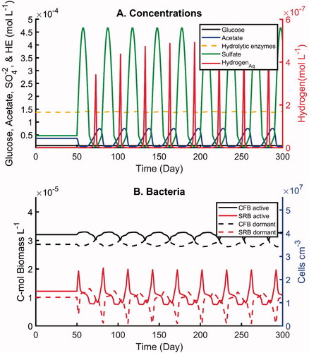
Figure 6. Simulations with imposed oscillations in sulfate concentration by one order of magnitude and 30-day periodicity: (A) concentrations of electron-donors and hydrolytic enzymes, (B) active and dormant bacterial biomasses. All concentrations are in moles carbon per unit volume pore water, except sulfate and dihydrogen which is given in moles per unit volume pore water.

For the simulation results presented here, the maximum sulfate concentration is set at 4.7×10⁻⁴mol L⁻¹ (i.e., one order of magnitude higher than the steady-state concentration of 4.7×10⁻⁵mol L⁻¹ in the baseline simulation) and the minimum sulfate concentration at 4.7×10⁻⁶mol L⁻¹ (i.e., an order of magnitude lower than the steady-state concentration). In other words, x in Equation 23(23a) $$\mathrm{THEN}\hspace{1em}\hspace{1em}y\left(t\right)=S\left(1+\left(x-1\right)\times \text{sin}\left(2\pi ft\right)\right),$$(23a) equals 10 (Figures 6, 7). Two different time periods are considered: 30 and 365 days (scenarios 7 and 8, Table 3). The imposed monthly and yearly periodicities bracket the seasonal fluctuations in hydrochemistry often observed in shallow aquifers (Scheytt 1997). In both scenarios, the concentrations of the aqueous constituents follow similar patterns with some notable differences (Figures 6(A), 7(A)). The acetate and dihydrogen concentrations drop to very low levels during times of peak sulfate concentrations, while they reach their maximum values when the sulfate concentration falls below 4.7 × 10⁻⁵mol L⁻¹. However, the rise of the acetate concentration under the low sulfate conditions is more gradual than for dihydrogen: dihydrogen peaks sharply when sulfate is at its lowest level. Differences between scenarios 7 and 8 include a lower and less symmetric acetate peak at the higher (monthly) frequency, dihydrogen peak values that are an order of magnitude smaller at the lower (yearly) frequency, and slightly more variability in the hydrolytic enzyme concentrations during the yearly sulfate fluctuations. While variations of the glucose concentration were observed in both scenarios, their amplitudes remained low.

Figure 7. Simulations with imposed oscillations in sulfate concentration by one order of magnitude and one-year periodicity: (A) concentrations of electron-donors and hydrolytic enzymes, (B) active and dormant bacterial biomasses. All concentrations are in moles carbon per unit volume pore water, except sulfate and dihydrogen which is given in moles per unit volume pore water.

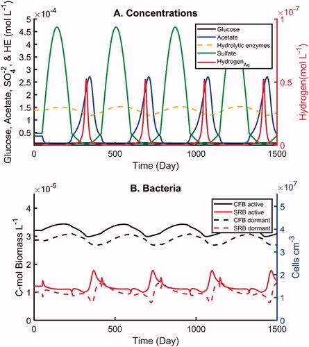
The microbial biomasses show distinct responses to the two imposed sulfate periodicities (Figures 6(B), 7(B)). In particular, the amplitude of the variations in active and dormant SRB is much greater under the monthly fluctuations in sulfate availability. When sulfate concentrations rise, the active SRB biomass increase seems to be largely fulfilled by activation of the dormant biomass compared to the formation of new cells (Figure 6(B)). Because of the higher contribution from interconversion between active and dormant cells, the temporal patterns of the corresponding biomasses closely mirror each other under the monthly periodicity (Figure 6(B)). Although opposite temporal trends for the active and dormant biomasses are also observed under the yearly oscillations, they no longer closely mirror each other (Figure 7(B)). This is best seen when considering the peaks in the active biomass. The corresponding drop in dormant biomass has a smaller magnitude and reaches its minimum earlier than the active biomass peak. Thus, additional biomass growth is needed to explain the amplitude of the active biomass peaks. In other words, when the period of the oscillations increases, biomass growth (and decay) becomes increasingly important in controlling the SRB biomasses. At the same time, this also reduces the amplitude of the biomass variations, as shown by comparing Figures 6(B), 7(B).

In both scenarios, when in a given cycle the sulfate concentrations start increasing the first response of the active SRB biomass is also to increase. However, the peak in active SRB biomass is reached while the sulfate concentration is still rising. In fact, by the time the sulfate concentration reaches its maximum, the active SRB biomasses have dropped back to values close to the steady-state biomasses. This is due to the drop in the concentrations of acetate and dihydrogen and, hence, the dwindling availability of energy and carbon substrates required by the SRB (Figures 6(A), 7(A)). That is, the activity of the SRB becomes limited by the rate at which the CFB is producing electron donors for the SRB.

The biomass variations of the CFB are relatively small compared to those experienced by the SRB. As for the SRB, however, there is a distinct difference between the temporal trends of active and dormant CFB under the two periodicities. At the higher monthly frequency, the active and dormant biomasses of the CFB mirror each other closely (Figure 6(B)). For the 1-year cycle in sulfate availability, however, there is a phase shift between active and dormant biomasses (Figure 7(B)). The CFB responds to the monthly sulfate fluctuations primarily by switching between the active and dormant states, while for the yearly fluctuations, biomass growth and decay play a greater role in the biomass changes. The CFB biomass oscillations seen in Figures 6(B), 7(B) are driven by the fluctuations in the concentrations of acetate and dihydrogen. The fermentation products affect the Gibbs energy production of the CFB through the reaction quotients of the catabolic pathways. Thus, in a given cycle, the active CFB biomass begins to decrease when acetate starts building up and reaches its minimum when the dihydrogen concentration peaks. The active CFB biomass is highest during the time of peak sulfate concentrations when the acetate and dihydrogen are at their lowest levels.

In contrast to the large fluctuations in the aqueous geochemistry of the modeled system, the amplitudes of the total (active plus dormant) biomass fluctuations of the CFB and SRB remained relatively small during the simulations. The dampened total biomass fluctuations are due to the ability of the cells to reversibly switch between active and dormant states. In other words, switching between active and dormant states confers resiliency to the community structure when faced with variations in catabolic energy supply.

Sensitivity analysis

As mentioned in the section Parameter values, many model parameters exhibit broad ranges or carry large uncertainties. We performed a global sensitivity analysis to determine the most important model parameters defining the steady-state microbial concentrations. This was done using the Fourier Amplitude Sensitivity Test (FAST) (Cukier et al. 1973; Saltelli et al. 1999). Two sensitivity indices were used to evaluate the dependence of model outcomes on the parameters: (1) the first-order sensitivity (denoted ‘first’), which evaluates the variance of the model output to a given parameter across a prescribed parameter range while keeping the other parameters constant, and (2) the total sensitivity (denoted ‘total’) that also includes all possible cross-contributions, in which the other parameters are scanned simultaneously over their respective ranges. Ranges of ±15% relative to the default values were considered for all the parameters in Table 1. The conditional variances obtained for a given parameter were normalized by the corresponding total variances, resulting in sensitivity indices ranging between zero and one. Figures 8, 9 show the first- and total-order sensitivity indices according to FAST. The larger the sensitivity indices, the more the model outcome is sensitive to the parameter value. Note that the sensitivity indices are shown as bar plots on a logarithmic scale.

Figure 8. Sensitivity analysis using Fourier Amplitude Sensitivity Test (FAST) with the total bacterial biomass (CFB plus SRB, active plus dormant) as the observable variable: ‘First’: first-order sensitivity index; ‘Total’: total sensitivity index. See text for details.

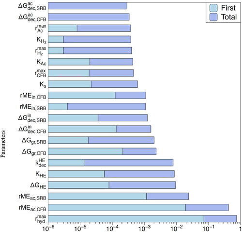
Figure 9. Sensitivity analysis using Fourier Amplitude Sensitivity Test (FAST) with the fraction of fermenting bacteria (CFB) as the observable variable: ‘First’: first-order sensitivity index; ‘Total’: total sensitivity index. See text for details.

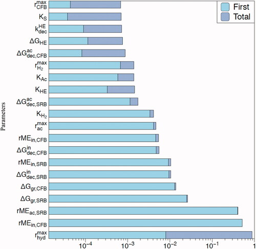
First, we used the total bacterial abundance (CFB plus SRB, active plus dormant) at a steady state as the observable variable computed by the model (Figure 8). Not surprisingly, the total bacterial biomass is most sensitive to the maximum hydrolysis rate $r_{\mathit{hyd}}^{\mathit{max}}$ because it controls the supply of the primary energy substrate (glucose) fueling the microbial community as a whole. In subsurface environments, $r_{\mathit{hyd}}^{\mathit{max}}$ reflects the abundance, reactivity, and accessibility of particulate organic matter. Values of $r_{\mathit{hyd}}^{\mathit{max}}$ are therefore expected to cover a very large range, given that even just the reactivity of natural organic matter alone already varies across several orders of magnitude (Van Cappellen and Gaillard 1996). Following $r_{\mathit{hyd}}^{\mathit{max}},$ the most sensitive parameters are the maintenance energy requirements of the active bacteria ($r_{{ME}_{ac}}$). This is also not unexpected as the maintenance requirements largely determine the energy demand side of the microbial community. Next in line are the parameters regulating the production and decay of hydrolytic enzymes, with only minor sensitivities for the remaining model parameters.

Second, we focused on the sensitivity of the community structure to variations in the model parameters using the fraction of CFB in the total steady-state biomass as the target observable. Again, $r_{\mathit{hyd}}^{\mathit{max}}$ and the maintenance energy requirements of active CFB and SRB emerge as the most sensitive parameters, followed by the Gibbs energies for growing new SRB and CFB cells (${\Delta G}_{gr,\mathit{SRB}},\mathrm{ }{\mathrm{ }\Delta G}_{gr,\mathit{CFB}}$). Overall, the sensitivity analysis highlights the need for more accurate estimations of the bioenergetics of maintenance and growth of subsurface microbial populations.

Concluding remarks

The proposed modeling approach provides a general framework for allocating the catabolic energy generated during the degradation of organic matter by subsurface microorganisms between producing extracellular hydrolytic enzymes, meeting cellular maintenance energy requirements, and growing new biomass. Imbalances between the production and consumption of energy by different functional groups of microorganisms are further accommodated by the reversible switching of cells between active and dormant states. The approach is applied to a hypothetical cellulose-degrading consortium comprising fermenting and sulfate-reducing bacteria. Particular attention is given to the cooperative interactions regulated by the thermodynamic feedbacks between the two microbial groups resulting from dynamic adjustments of the catabolic Gibbs energy production.

The steady and non-steady state simulations illustrate how bioenergetics shape both the community structure and aqueous geochemical conditions in the modeled consortium. In future work, the modeling framework can be expanded by incorporating additional energy expenditures and regulating processes, to simulate more complex geomicrobial systems. A key strength of the proposed kinetic-thermodynamic modeling approach is the ability to formulate quantitative hypotheses about the functioning of microbial communities in subsurface environments. These hypotheses can then be verified in controlled laboratory experiments or the field through the acquisition of in situ data, including multi-omics data sets.

Disclosure statement

No potential conflict of interest was reported by the authors.

Additional information

Funding

This research was funded by Deutsche Forschungsgemeinschaft (DFG) in the framework of the international research training group ‘Integrated Hydrosystem Modelling’ under grant GRK 1829, the Canada Excellence Research Chair (CERC) in Ecohydrology at the University of Waterloo, and the Canada First Research Excellence Fund (CFRF) through the Global Water Futures (GWF) program.

References

- Amenabar MJ, Shock EL, Roden EE, Peters JW, Boyd ES. 2017. Microbial substrate preference dictated by energy demand rather than supply. Nat. Geosci. 10:577–581. doi:https://doi.org/10.1038/NGEO2978
- Anderson TH, Domsch KH. 1985. Determination of ecophysiological maintenance carbon requirements of soil microorganisms in a dormant state. Biol Fertil Soils 1:81–89.
- Arora B, Cheng Y, King E, Bouskill N, Brodie E. 2017. Modeling microbial energetics and community dynamics. Handb Met Interact Bioremediation, 1st edition; CRC Press; 445–454.
- Bajracharya B, Lu C, Cirpka OA. 2014. Modeling substrate-bacteria-grazer interactions coupled to substrate transport in groundwater. Water Resour Res 50(5):4149–4162.
- Béguin P, Aubert JP. 1994. The biological degradation of cellulose. FEMS Microbiol Rev 13(1):25–58.
- Belli KM, DiChristina TJ, Van Cappellen P, Taillefert M. 2015. Effects of aqueous uranyl speciation on the kinetics of microbial uranium reduction. Geochim Cosmochim Acta 157:109–124.
- Bezerra RMF, Dias AA. 2004. Discrimination among eight modified Michaelis-Menten kinetics models of cellulose hydrolysis with a large range of substrate/enzyme ratios: inhibition by cellobiose. Appl Biochem Biotechnol. 112(3):173–184.
- Brock AL, Kästner M, Trapp S. 2017. Microbial growth yield estimates from thermodynamics and its importance for degradation of pesticides and formation of biogenic non-extractable residues. SAR QSAR Environ. Res. 28:629–650. doi:https://doi.org/10.1080/1062936X.2017.1365762
- Canfield DE, Kristensen E, Thamdrup B. 2005. 2 Structure and growth of microbial populations. Adv Mar Biol 48:23–64.
- Christensen TH, Bjerg PL, Banwart SA, Jakobsen R, Heron G, Albrechtsen HJ. 2000. Characterization of redox conditions in groundwater contaminant plumes. J Contam Hydrol 45(3–4):165–241.
- Cukier RI, Fortuin CM, Shuler KE, Petschek AG, Schaibly JH. 1973. Study of the sensitivity of coupled reaction systems to uncertainties in rate coefficients. I Theory. J Chem Phys 59(8):3873–3878.
- Dale A, Regnier P, Van Cappellen P. 2006. Bioenergetic controls on anaerobic oxidation of methane (AOM) in coastal marine sediments: a theoretical analysis. Am J Sci 306(4):246–294.
- Del Giorgio P, Cole JJ. 1998. Bacterial growth efficiency in natural aquatic systems. Annu Rev Ecol Syst 29(1998):503–541.
- Demirel Y, Sandler SI. 2002. Thermodynamics and bioenergetics. Biophys Chem 97(2–3):87–111.
- Detmers J, Schulte U, Strauss H, Kuever J. 2001. Sulfate reduction at a lignite seam: microbial abundance and activity. Microb Ecol 42(3):238–247.
- Eastman JA, Ferguson JF. 1981. Solubilization of particulate organic carbon during the acid phase of anaerobic digestion. J Water Pollut Control Fed 53:352–366.
- German DP, Marcelo KRB, Stone MM, Allison SD. 2012. The Michaelis-Menten kinetics of soil extracellular enzymes in response to temperature: a cross-latitudinal study. Glob Chang Biol 18(4):1468–1479.
- Griebler C, Lueders T. 2009. Microbial biodiversity in groundwater ecosystems. Freshw Biol 54(4):649–677.
- Hall SJ, Treffkorn J, Silver WL. 2014. Breaking the enzymatic latch: Impacts of reducing conditions on hydrolytic enzyme activity in tropical forest soils. Ecol Soc Am. 95:2964–2973. doi:https://doi.org/10.1890/13-2151.1
- Heijnen JJ, Dijken JP. 1992. In search of a thermodynamic description of biomass yields for the chemotrophic growth of microorganisms. Biotechnol Bioeng 39(8):833–852.
- Hoehler TM, Alperin MJ, Albert DB, Martens CS. 1998. Thermodynamic control on hydrogen concentrations in anoxic sediments. Geochim Cosmochim Acta 62(10):1745–1756.
- Hoehler TM, Jørgensen BB. 2013. Microbial life under extreme energy limitation. Nat Rev Microbiol 11(2):83–94.
- Hoehler TM. 2004. Biological energy requirements as quantitative boundary conditions for life in the subsurface. Geobiology 2(4):205–215.
- Hoijnen JJ, van Loosdrecht MCM, Tijhuis L. 1992. A black box mathematical model to calculate auto- and heterotrophic biomass yields based on Gibbs energy dissipation. Biotechnol. Bioeng. 40:1139–1154. doi:https://doi.org/10.1002/bit.260401003
- Ingvorsen K, Zehnder JB, Jørgensen BB. 1984. Kinetics of sulphate and acetat uptake by Desulfobacter postgatei. Appl Environ Microbiol 47(2):403–408.
- Jin Q, Bethke CM. 2005. Predicting the rate of microbial respiration in geochemical environments. Geochim Cosmochim Acta 69(5):1133–1143.
- Jin Q, Bethke CM. 2007. The thermodynamics and kinetics of microbial metabolism. Am J Sci 307(4):643–677.
- Jin Q, Bethke CM. 2009. Cellular energy conservation and the rate of microbial sulfate reduction. Geology 37:1027–1030.
- Jin Q, Kirk MF. 2018. pH as a primary control in environmental microbiology: 1. Thermodynamic perspective. Front Environ Sci 6:21.
- Jones SE, Lennon JT. 2010. Dormancy contributes to the maintenance of microbial diversity. Proc Natl Acad Sci USA 107(13):5881–5886.
- Jurtshuk P. 1996. Bacterial metabolism. In: Baron, S, editor. Medical Microbiology. Galveston: University of Texas Medical Branch at Galveston.
- Kempes CP, van Bodegom PM, Wolpert D, Libby E, Amend J, Hoehler T. 2017. Drivers of bacterial maintenance and minimal energy requirements. Front Microbiol 8:31.
- Khosrovi B, Macpherson R, Miller JD. 1971. Some observations on growth and hydrogen uptake by Desulfovibrio vulgaris. Arch Mikrobiol 80(4):324–337.
- Kim DS, Fogler HS. 2000. Biomass evolution in porous media and its effects on permeability under starvation conditions. Biotechnol Bioeng 69(1):47–56.
- Kleman G, Strohl W. 1994. Acetate metabolism by Escherichia coli in high-cell-density fermentation. Appl Environ Microbiol 60(11):3952–3958.
- Kneeshaw TA, Mcguire JT, Cozzarelli IM, Smith EW. 2011. In situ rates of sulfate reduction in response to geochemical perturbations. Ground Water 49(6):903–913.
- LaRowe DE, Dale AW, Amend JP, Van Cappellen P. 2012. Thermodynamic limitations on microbially catalyzed reaction rates. Geochim Cosmochim Acta 90:96–109.
- Lennon JT, Jones SE. 2011. Microbial seed banks: the ecological and evolutionary implications of dormancy. Nat Rev Microbiol 9(2):119–130.
- Leschine SB. 1995. Cellulose degradation in anaerobic environments. Annu Rev Microbiol 49:399–426.
- Liu JS, Vojinović V, Patiño R, Maskow T, von Stockar U. 2007. A comparison of various Gibbsenergy dissipation correlations for predicting microbial growth yields. Thermochim. Acta 458:38–46. doi:https://doi.org/10.1016/j.tca.2007.01.016
- Lovley DR, Chapelle FH. 1995. Deep subsurface microbial processes. Rev Geophys 33(95):365–381.
- Lovley DR, Goodwin S. 1988. Hydrogen concentrations as an indicator of the predominant terminal electron-accepting reactions in aquatic sediments.
- Lovley DR, Phillips EJP. 1989. Requirement for a microbial consortium to completely oxidize glucose in Fe(III)-reducing sediments. Appl Environ Microbiol 55(12):3234–3236.
- Lynd LR, Weimer PJ, Zyl WH, Van IS. 2002. Microbial cellulose utilization: fundamentals and biotechnology. Microbiol Mol Biol Rev 66(3):506–577.
- Moorhead DL, Rinkes ZL, Sinsabaugh RL, Weintraub MN. 2013. Dynamic relationships between microbial biomass, respiration, inorganic nutrients and enzyme activities: informing enzyme-based decomposition models. Front Microbiol 4:223.
- Morita RY. 1988. Bioavailability of energy and its relationship to growth and starvation survival in nature. Can J Microbiol 34(4):436–441.
- Novelli PC, Michelson AR, Scranton M, Banta G, Hobbie J, Howarth R. 1988. Hydrogen and acetate cycling in two sulfate-reducing sediments: Buzzards Bay and Town Cove, Mass. Geochim Cosmochim Acta 52(10):2477–2486.
- Pallud C, Van Cappellen P. 2006. Kinetics of microbial sulfate reduction in estuarine sediments. Geochim Cosmochim Acta 70(5):1148–1162.
- Payn RA, Helton AM, Poole GC, Izurieta C, Burgin AJ, Bernhardt ES. 2014. A generalized optimization model of microbially driven aquatic biogeochemistry based on thermodynamic, kinetic, and stoichiometric ecological theory. Ecol Modell 294:1–18.
- Pérez J, Muñoz-Dorado J, De La Rubia T, Martínez J. 2002. Biodegradation and biological treatments of cellulose, hemicellulose and lignin: an overview. Int Microbiol 5(2):53–63.
- Phelps TJ, Murphy EM, Pfiffner SM, White DC. 1994. Comparison between geochemical and biological estimates of subsurface microbial activities. Microb Ecol 28(3):335–349.
- Plugge CM, Zhang W, Scholten JCM, Stams AJM. 2011. Metabolic flexibility of sulfate-reducing bacteria. Front Microbiol 2:81.
- Popovic M. 2019. Thermodynamic properties of microorganisms: determination and analysis of enthalpy, entropy, and Gibbs free energy of biomass, cells and colonies of 32 microorganism species. Heliyon 5(6):e01950.
- Reis MA, Almeida JS, Lemos PC, Carrondo MJ. 1992. Effect of hydrogen sulfide on growth of sulfate reducing bacteria. Biotechnol Bioeng 40(5):593–600.
- Resat H, Bailey V, McCue LA, Konopka A. 2012. Modeling microbial dynamics in heterogeneous environments: growth on soil carbon sources. Microb Ecol 63(4):883–897.
- Rickard D, Luther GW. 1997. Kinetics of pyrite formation by the H2S oxidation of iron (II) monosulfide in aqueous solutions between 25 and 125 °C: the mechanism. Geochim Cosmochim Acta 61(1):135–147.
- Roden EE. 2008. Microbiological controls on geochemical kinetics 1: fundamentals and case study on microbial Fe(III) oxide reduction. In: Brantley, SL, Kubicki, JD, White, AF, editors. Kinetics of Water-Rock Interactions. New York: Springer, p335–415.
- Roden EE, Jin Q. 2011. Thermodynamics of microbial growth coupled to metabolism of glucose, ethanol, short-chain organic acids, and hydrogen. Appl Environ Microbiol 77(5):1907–1909.
- Roden EE, Wetzel RG. 2002. Kinetics of microbial Fe(III) oxide reduction in freshwater wetland sediments. Limnol Oceanogr 47(1):198–211.
- Roels JA. 1980. Application of macroscopic principles to microbial metabolism. Biotechnol Bioeng 103(1):2–59.
- Rotter BE, Barry DA, Gerhard JI, Small JS. 2008. Parameter and process significance in mechanistic modeling of cellulose hydrolysis. Bioresour Technol 99(13):5738–5748.
- Russell J, Cook G. 1995. Energetics of bacterial growth: balance of anabolic and catabolic reactions. Microbiol Rev 59(1):48–62.
- Russell JB. 1986. Heat production by ruminal bacteria in continuous culture and its relationship to maintenance energy. J Bacteriol 168(2):694–701.
- Saltelli A, Tarantola S, Chan KP-S. 1999. A quantitative model-independent method for global sensitivity analysis of model output. Technometrics 41(1):39–56.
- Scheibe TD, Mahadevan R, Fang Y, Garg S, Long PE, Lovley DR. 2009. Coupling a genome-scale metabolic model with a reactive transport model to describe in situ uranium bioremediation. Microb Biotechnol. 2:274–286. doi:https://doi.org/10.1111/j.1751-7915.2009.00087.x
- Scheibe TD, Fang Y, Murray CJ, Roden EE, Chen J, Chien YJ, Brooks SC, Hubbard SS. 2006. Transport and biogeochemical reaction of metals in a physically and chemically heterogeneous aquifer. Geosphere 2(4):220–235.
- Scheytt T. 1997. Seasonal variations in groundwater chemistry near Lake Belau, Schleswig-Holstein, Northern Germany. Hydrogeology 5(2):86–95.
- Shampine LF, Reichelt MW. 1997. The MATLAB ODE Suite. SIAM J Sci Comput. 18(1):1–22.
- Sinsabaugh RL, Follstad Shah JJ. 2012. Ecoenzymatic stoichiometry and ecological theory. Annu Rev Ecol Evol Syst. 43(1):313–343.
- Sinsabaugh RL, Follstad Shah JJ. 2012. Ecoenzymatic stoichiometry and ecological theory. Annu. Rev. Ecol. Evol. Syst. 43:313–343. doi:https://doi.org/10.1146/annurev-ecolsys-071112-124414
- Small J, Nykyri M, Helin M, Hovi U, Sarlin T, Itävaara M. 2008. Experimental and modelling investigations of the biogeochemistry of gas production from low and intermediate level radioactive waste. Appl Geochem 23(6):1383–1418.
- Smeaton CM, Van Cappellen P. 2018. Gibbs energy dynamic yield method (GEDYM): predicting microbial growth yields under energy-limiting conditions. Geochim Cosmochim Acta 241:1–16.
- Stolpovsky K, Martinez-Lavanchy P, Heipieper HJ, Van Cappellen P, Thullner M. 2011. Incorporating dormancy in dynamic microbial community models. Ecol Modell 222(17):3092–3102.
- Thullner M, Regnier P. 2019. Microbial controls on the biogeochemical dynamics in the subsurface. Rev Miner Geochem 85(1):265–302.
- Tiehm A, Nickel K, Neis U. 1997. The use of ultrasound to accelerate the anaerobic digestion of sewage sludge. Water Sci Technol 36:121–128.
- Tijhuis L, Van Loosdrecht MC, Heijnen JJ. 1993. A thermodynamically based correlation for maintenance Gibbs energy requirements in aerobic and anaerobic chemotrophic growth. Biotechnol Bioeng 42(4):509–519.
- Van Bodegom P. 2007. Microbial maintenance: a critical review on its quantification. Microb Ecol 53(4):513–523.
- Van Cappellen P, Gaillard JF. 1996. Biogeochemical dynamics in aquatic sediments. Rev Miner 34:335–376.
- Van Walsum GP, Lynd LR. 1998. Allocation of ATP to synthesis of cells and hydrolytic enzymes in cellulolytic fermentative microorganisms: bioenergetics, kinetics, and bioprocessing. Biotechnol Bioeng 58:316–320.
- VanBriesen JM. 2002. Evaluation of methods to predict bacterial yield using thermodynamics. Biodegradation 13(3):171–190.
- Vavilin VA, Fernandez B, Palatsi J, Flotats X. 2008. Hydrolysis kinetics in anaerobic degradation of particulate organic material: an overview. Waste Manag 28(6):939–951.
- Wang G, Post W, Mayes M. 2013. Development of microbial-enzyme-mediated decomposition model parameters through steady-state and dynamic analyses.
- Wilson DB. 2008. Three microbial strategies for plant cell wall degradation. Ann N Y Acad Sci 1125:289–297.
- Wilson DB. 2009. Cellulases and biofuels. Curr Opin Biotechnol 20(3):295–299.
- Wilson DB. 2011. Microbial diversity of cellulose hydrolysis. Curr Opin Microbiol 14(3):259–263.
- Wrighton KC, Castelle CJ, Wilkins MJ, Hug LA, Sharon I, Thomas BC, Handley KM, Mullin SW, Nicora CD, Singh A, et al. 2014. Metabolic interdependencies between phylogenetically novel fermenters and respiratory organisms in an unconfined aquifer. ISME J 8(7):1452–1463.
- Zhang Y-HP, Lynd LR. 2005. Cellulose utilization by Clostridium thermocellum: bioenergetics and hydrolysis product assimilation. Proc Natl Acad Sci USA 103(39):9429–9430.
- Zhuang K, Izallalen M, Mouser P, Richter H, Risso C, Mahadevan R, Lovley DR. 2011. Genome-scale dynamic modeling of the competition between Rhodoferax and Geobacter in anoxic subsurface environments. ISME J. 5:305–316. doi:https://doi.org/10.1038/ismej.2010.117