How can a few streamflow measurements help to predict daily hydrographs at almost ungauged sites?

Abstract

Available data from nearby gauging stations can provide a great source of hydrometric information that is potentially transferable to an ungauged site. Furthermore, streamflow measurements may even be available for the ungauged site. This paper explores the potential of four distance-based regionalization methods to simulate daily hydrographs at almost ungauged pollution-control sites. Two methods use only the hydrological information provided by neighbouring catchments; the other two are new regionalization methods parameterized with a limited number of streamflow data available at the site of interest. Based on a network of 149 streamgauges and 21 pollution-control sites located in the Upper Rhine-Meuse area, the comparative assessment demonstrates the benefit of making available point streamflow measurements at the location of interest for improving quantitative streamflow prediction. The advantage is moderate for the prediction of flow types (stormflow, recession flow, baseflow) and pulse shape (duration of rising limb and falling limb).

Editor Z.W. Kundzewicz; Associate editor A. Viglione

Résumé

Les données disponibles aux stations hydrométriques voisines constituent une source d’information potentiellement transférable en un site non jaugé. De surcroît, dans certaines situations chanceuses, des jaugeages épisodiques y ont été réalisés. Cet article explore le potentiel de quatre méthodes de régionalisation par proximité destinées à simuler l’hydrogramme journalier en des sites de contrôle de la pollution peu jaugés. Deux des quatre méthodes (la méthode de la ‘carte de corrélation’ et la méthode par voisinage géographique) n’exploitent que l’information hydrologique (hydrogrammes observés ou simulés) fournie par les bassins voisins pour reconstituer le débit journalier. Les deux autres (la méthode par paramétrisation discrète des modèles hydrologiques et la méthode débit–débit) constituent des approches originales et sont paramétrées en utilisant en outre, les données de débits ponctuels échantillonnées au point-cible. L’analyse comparative effectuée à partir d’un réseau de 149 stations hydrométriques et 21 stations des réseaux de contrôle de surveillance (RCS) démontre un gain substantiel d’efficacité du processus de régionalisation du débit journalier grâce à l’information hydrométrique ponctuelle disponible au point-cible. En revanche, ce gain est plus modéré pour prédire les types d’écoulement (écoulement de crue, décrue, tarissement) et la durée des phases hydrologiques.

Key words:

• point flow measurements
• regionalization
• neighbourhood
• map correlation method
• spatial proximity
• discrete parameterization of hydrological models
• streamflow–streamflow method
• ungauged catchment
• pollution-control site

Mots clefs:

• débits ponctuels
• régionalisation
• voisinage
• méthode de la « carte de corrélation »
• proximité spatiale
• paramétrisation discrète des modèles hydrologiques
• méthode débit-débit
• bassin non jaugé
• site de contrôle de la pollution

INTRODUCTION

Research on regionalization in hydrology has experienced innovative developments since the last decade, especially through the Predictions in Ungauged Basins (PUB) initiative (2003–2012) of the International Association of Hydrological Sciences (Hrachowitz et al. 2013). During this decade of intensive research, attention was mainly focused on predictions of streamflow signatures (i.e. temporal patterns of catchment streamflow response) for catchments where no streamflow data are available. For that purpose, different regionalization methods were tested and assessed throughout the world over a wide range of climates, environments and hydrological processes (Parajka et al. 2013).

However, relatively few papers have dealt with the use of non-continuous streamflow data series for the parameterization of regionalization methods. Although, in many parts of the world long streamflow time series are absent, there are often short time series, or at least non-continuous flow measurements, available in the region of interest. They may be very informative in helping to understand catchment behaviour and to predict continuous hydrographs. In the field of rainfall–runoff modelling, Blöschl (2005) claims that “…the best way to handle the issue of rainfall–runoff modelling in ungauged catchments would be to install a stream gauge. Indeed, limited or incomplete data can still be extremely valuable because one can use it to constrain model calibrations”. Hence, even though technical and/or financial constraints may prevent a staff-gauge station being set up and monitored to get the hydrological information needed for practical purposes, an alternative way may be to gauge the ungauged catchments through a limited number of field measurements (Perrin et al. 2007, Seibert and Beven 2009).

In France, for example, some intensive point flow measurement campaigns have been coordinated by the Rhine-Meuse Water Authority over the last two decades (e.g. François and Sary 1990, Decloux and Sary 1991). This source of data may greatly improve the knowledge and estimation of low flows or flood events at ungauged sites (Chopart and Sauquet 2008). It is, however, insufficient to reconstruct the hydrological context of surface water quality samples collected on behalf of the Water Framework Directive (2000/60/EC) monitoring programme.

MAKING RIVER WATER QUALITY DATA MORE MEANINGFUL

Table 1 shows the signs of the relationship generally observed between nitrate concentrations (daily values and time variability) in river flows and some relevant hydrological variables: antecedent daily river flow, daily river flow, baseflow index (e.g. Clausen et al. 1999, Guillaud and Bourriel 2007). In light of these co-variations, there is clearly a link between river flows, hydrogeological characteristics of catchments and pollutants loads in the stream network.

Table 1 Common signs of correlation between nitrate concentrations [NO₃] in river flows (daily values and time variability) and some hydrological variables: antecedent daily river flow (Q_j–i), daily river flow (Q_j) and baseflow index (BFI). CV: coefficient of variation.

	Qj–i	Qj	BFI
[NO3]j	(+)	(−)
CV [NO3]j			(−)

Such findings were generally obtained through cross-analysis of water quality data and continuous hydrological time series collected for a few years. When streamflow data are missing, or poorly measured at the location of interest, it is difficult, if not impossible, for water managers to calculate pollutant loads and interpret water quality data and trends on pollutant indicators (Burt et al. 2010). In that respect, reconstructing continuous hydrological information for a few “benchmark” sites is crucial in terms of enhancing process understanding and identifying system lags. Hydrological information can give valuable data on the overall types of water pathways, processes and streamflow dynamics in a catchment. This will contribute to the understanding of short-term fluctuations in pollutant concentrations recorded in river flows during particularly influential hydrological events.

The scope of this paper is to evaluate, through a regional comparative assessment of distance-based regionalization methods, the potential of point flow measurements for reducing uncertainty in the prediction of daily hydrographs at almost ungauged pollution-control sites. This comparative assessment is motivated by the fact that outcomes of regionalization methods can be disparate for a given location of interest, and subject to variation according to their parameterization scheme (Drogue et al. 2002, Kay et al. 2006).

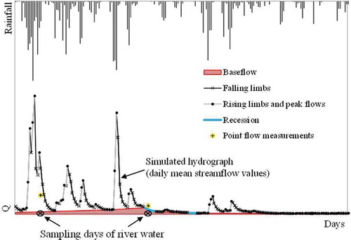
The ultimate goal is to provide a decision-making support tool for predicting daily streamflow and flow types (stormflow, recession flow, baseflow) at water quality monitoring locations based on the available data (Fig. 1).

Fig. 1 Reconstruction and segmentation of a daily hydrograph at an almost ungauged pollution-control site: a contribution to meta-analysis of river quality data sampling. Note that uncertainty bounds should bracket the simulated hydrograph (not shown). Segmentation was performed according to the procedure described in the section “Comparative Assessment”.

METHODS OF REGIONALIZATION

The most intuitive way to transfer hydrological information from one catchment to another that is treated as ungauged is to identify similar or proxy catchments, be it in terms of location or behaviour (He et al. 2011). In this paper, we compare both approaches through distance-based regionalization methods, while adapting their parameterization according to the available hydrological data at the location of interest. Two types of method were tested:

• Reference “naïve” and intuitive methods parameterized only with the hydrological information (streamflow data or simulated hydrographs) provided by the neighbour catchments: we selected the map correlation method (distance is estimated through correlation fields) and the spatial proximity method (distance is calculated between catchment centroids). These two popular methods may be viewed as “benchmark” methods.

• New methods parameterized according to the distance between point flow measurements available at the location of interest and hydrological information (streamflow data or simulated hydrographs) provided by the neighbouring catchments. In this case, the distance between catchments is considered as a metric of hydrological similarity between donor catchments and almost ungauged receiver catchments.

The map correlation (MC) method

This method has been recently evaluated on a set of US catchments by Archfield and Vogel (2010). It basically relies on the fact that the selection of the nearest streamgauge as a reference streamgauge for an ungauged catchment is not always the streamgauge having the highest correlated daily streamflow values, even in a relatively homogeneous study region. The conceptual framework and the basic assumptions underlying the method are as follows (Woods and Sivapalan 1999, Archfield and Vogel 2010):

1. Streamflow exists at any location.

2. It is possible to estimate cross‐correlation between the daily streamflows at a streamgauge and an ungauged site for any location in the study area.

3. The study area is not limited by regions of homogeneity or other hydrologic boundaries.

4. A minimum number of streamgauges in the network is necessary for the geostatistical methods to be reliable.

5. The records at each of the streamgauges must be coincident with other streamgauges in the study area for a sufficiently long period such that estimates of correlation are representative of the full range of daily streamflow values for the streamgauges in the study region.

6. The cross-correlation values are isotropic across the study region.

To determine if a spatial covariance structure in the cross-correlation values exists, a variographic analysis is implemented for each streamgauge in the study area. By interpolating cross-correlation values with ordinary kriging it is possible to obtain a continuous map of correlation between a given streamgauge and the surrounding area. This correlation map shows the spatial distribution of the correlation between a given streamgauge and any other location of interest in the study region. Once all the correlation maps are produced for all the streamgauges within the study area, one can select the most correlated reference catchment (i.e. the neighbour catchment) for a given ungauged catchment simply according to its location.

In this study, as the streamgauge network is quite dense (typically 1 streamgauge per 250 km²), we decided to implement a modified version of the MC method allowing multiple neighbours. We assigned a rank to the donor catchments based on their correlation to the target site: the first neighbour is that most correlated to the flow of the target catchment over the period of interest, and so on. Then a weighted linear combination of streamflow time series was tested with, successively, one to 20 members, and the best combination retained according to our performance criterion (C2M_√Q; see “Comparative Assessment” Section). The weights are proportional to the correlation coefficients of the donor catchments.

Even though this method does not use point flow measurements, it was selected as being simple in essence (selecting neighbouring catchments according to their area of influence) and straightforward for the purpose of interpolating streamflow time series.

The spatial proximity (SP) method

This method is very intuitive, relying on the assumption that close catchments will exhibit similar behaviour due to the similarity of their environments and climate. Ungauged catchments are modelled with model parameters calibrated for geographical neighbours and transferred to the location of interest. When a dense network of gauging stations is available (typically 1 streamgauge per 500 km²) and for temperate climates, this method has proved to be the best solution for regionalization of daily hydrographs (Parajka et al. 2013). The selection of the neighbour catchments is usually based on the Euclidean distance between catchment centroids.

Assuming n donor catchments, streamflow for day j is computed as:

(1)

where is the resulting daily streamflow hydrograph for the location of interest k, f_k is the input data (P and PET) of the catchment at outlet k, is the daily streamflow simulated with the vector of calibrated parameters θ_i of donor catchment i and input data f_k.

The information provided by neighbour catchments can be combined in two ways (McIntyre et al. 2005, Oudin et al. 2008):

1. by averaging the parameters of the neighbour catchments before computing the streamflow at the location of interest; or

2. by averaging the hydrographs simulated at the location of interest with the calibrated parameters of the neighbour catchments.

The discrete parameterization (DISP) method considering point flow data at the location of interest

The basics of the DISP approach were introduced by Perrin et al. (2008). It is similar to the SP methods and uses the same prior hydrological information from donor catchments: a library of previously calculated parameters calibrated on gauged catchments. The difference between DISP and SP lies in the fact that, for the SP method, the distance is computed in the space of geographical neighbours, whereas in the DISP method, the distance is computed in the space of hydrological neighbours. The latter are identified according to the model error between streamflow simulations obtained with donor catchment parameters and streamflow simulation obtained with an existing parameter set at the location of interest.

Here, we use a modified version of DISP proposed by Rojas-Serna et al. (submitted). With this new approach, selection of donor catchments is performed according to a “hybrid” distance combining a geographical distance and a “hydrological” distance between streamflow simulations and flow “observations” at the location of interest. The first step consists of calculating a rank for each donor catchment k as follows:

(2)

where r_k is the composite rank of the kth parameter set in the library and α is a weighting coefficient (varying between 0 and 1). The latter expresses the relative importance, in the calculation of the composite rank, given to the distance between the donor catchment k and the target catchment (r_k^geo) compared to the one given to hydrological similarity between the donor catchment k and the target catchment (r_k^hydro). The optimum value of α needs to be determined empirically. For α = 1, the method is similar to the SP approach; for α = 0, the method only uses point flow information. The composite rank r_k takes values of between 1 and p, where p denotes the number of predefined optima in the library. The value of r_k^geo is based on the Euclidean distance between catchment centroids while that of r_k^hydro is based on the following metric computed for each date j with point flow measurements:

(3)

where error_k,j is the root mean square error computed for the donor catchment k, Q_k,j is the simulated streamflow value at the outlet of the donor catchment k, and Q_r,j is the observed streamflow value at the outlet of the receiver catchment r. The square root transformed streamflows are used to give less importance to high streamflow values (floods) in the calculation of the error metric (Oudin et al. 2006).

Once the donor catchments are ranked according to equation (2), the second step is to compute streamflow for day j using equation (1). The optimal number of neighbour catchments and dates with point flow measurement should be evaluated through a sensitivity study.

The streamflow–streamflow (Q–Q) method considering point flow data at the location of interest

In a recent paper, Andréassian et al. (2012) demonstrate the added value of using neighbour catchments (NCs) for simulation of daily and hourly streamflow time series. They argue that a NC can be viewed as a full-scale model for a given catchment. With this perspective, there is no reason to think that errors of NC models (i.e. Nature’s own model) will be higher than those of rainfall–runoff models (i.e. human designed models).

Instead of only looking at one reference streamgauge, as in the time-honoured paired-catchment approach (the historical root of the MC method), the NC approach enables streamflow time series to be simulated at daily or hourly time steps based on streamflow time series observed at the outlet of one, or several, NC(s).

The Q–Q method is a combination of the DISP and MC approaches. It is applicable at the outlet of a catchment when point gauging records are available. The selection of NC is based on the same metric as the one used for DISP (see equation (3)). Simulated hydrographs are replaced by streamflow series observed at the outlet of the donor catchments. Again, the optimal number of point flow measurements should be evaluated through a sensitivity study.

Assuming n neighbour catchments, streamflow for time step j is computed as follows:

(4)

where is the simulated streamflow at the outlet of catchment k, and Q_i,j is the observed streamflow at the outlet of catchment i. The number of NCs, n, should be optimized through a sensitivity study. The weights assigned to the streamflow values of the NCs are calculated as the proportion of error of each NC to the total amount of prediction error, i.e.:

(5)

where w_k is the weight assigned to the NC k, m is the number of dates with point flow measurements, and n is the optimal number of NCs (see equation (4)). Equation (5) gives the highest weight to the streamflow time series having the closest streamflow values to point flow values observed at the outlet of the receiver catchment.

COMPARATIVE ASSESSMENT

Reconstruction of daily streamflow time series

The efficiency of each regionalization scheme was assessed through the bounded version of the Nash-Sutcliffe (NS) coefficient (Mathevet et al. 2006), computed on the square root of the daily streamflow values for the same reasons mentioned above. The criterion of efficiency is written as:

(6)

where NS is the Nash-Sutcliffe coefficient and is the square root transformed daily streamflow values. This C2M criterion takes values of between –1 and 1. A zero value indicates that the regionalization method is no more efficient than a naïve model simulating at each time step the daily streamflow value as the mean of the daily values. A value of 1 means that the regionalization method is capable of perfectly simulating the observed streamflow values. Note that computing the C2M criterion leads to lower values than the NS coefficient (e.g. a NS value of 0.8 corresponds to a C2M value of 0.666).

We used the leave-one-out cross-validation procedure to test the efficiency of the regionalization methods, each of the selected gauged sites being treated as ungauged. All the regionalization schemes were tested with daily area-normalized streamflow values.

Reconstruction of flow types and pulse shape

Quantitative hydrological information is not the only useful source of information for water quality data mining. Knowing flow types and pulse shape (duration of rising limb and falling limb) for a number of pollution-control sites could also give a general overview of the actual and eventually contributing flow processes in a catchment when surface water sampling has occurred. This is why we also evaluated the ability of the four distance-based regionalization schemes to reproduce observed flow types and pulse shape at the daily time step. With this aim, we discretized the simulated and observed hydrographs into three parts (see Fig. 1).

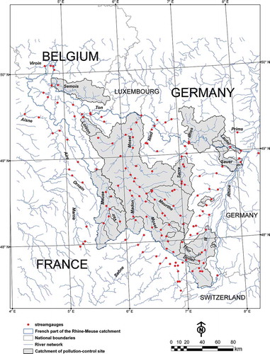
Fig. 2 Location of the 149 streamgauges and the 21 catchments of pollution-control sites used in this study.

Rising limb streamflows (including peak flows) and falling limb streamflows occurred, respectively, when:

(7)

and

(8)

where Q_k,j is the streamflow for day j at the outlet of catchment k and Q_k,j–1 is the streamflow for the previous day.

To identify sequences of baseflow data, we used the following empirical procedure:

1. The sequence should consist of at least 5 consecutive days.

2. Daily rainfall amount should not exceed 1 mm/d.

3. The initial streamflow value of the recession sequence (Q₀ at t = 0) should be less than the annual mean streamflow.

4. A lag time, T, is used as a first guess to define Q₀ at t = 0; T is obtained according to:

   (9)
   where A is the drainage area of the catchment(in km²).

5. As equation (7) is not optimal for defining Q₀, due to variations in physical characteristics of catchments, a regression line is additionally adjusted to the last streamflows of the recession sequence. Then, Q₀ is obtained through a retrospective calculation from the end of the recession sequence to the last ratio satisfying the inequality:

   (10)

where is the estimated daily baseflow for day j at the outlet of catchment k through the regression line.

This procedure was proposed by Lang and Gille (2006) and validated on numerous catchments within the study area. In case of ex aequo, the phase of the previous day is assigned to the current day.

The method outputs were classified for the three parts of the hydrograph. An index of agreement was defined as:

(11)

where C is a co-occurrence indicator taking a value of 1 in the case of agreement and 0 in the opposite case, Count is a function which counts the number of occurrences of a given phase of the hydrograph, is the ith occurrence of a given simulated phase at the outlet of catchment k, p_k,i is the ith occurrence of a given observed phase at the outlet of catchment k, and n is the number of time steps. The value of IA ranges from 0 (i.e. no agreement) to 100% (i.e. perfect agreement).

STUDY AREA, DATA AND MODEL

The region of interest has an area of approximately 38 000 km² (Fig. 2). It includes the French part of the upper Meuse, Mosel and Rhine catchments. The topography is characterized by the presence of cuestas and middle mountain areas (Ardennes, Eifel, Hunsrück, Vosges). The highest rainfall amounts are found in the southern parts of the Vosges (up to 2300 mm/year on average).

The Vosges Mountains, because of their north–south axis and their elevation (maximum of around 1400 m a.s.l), induce a mesoscale alteration of the climate, resulting in a quick transition between an oceanic type prevailing on the Vosges mountains and a continental type prevailing in the Rhine Valley.

The hydro-meteorological dataset refers to the period 1990–2009. Daily unregulated streamflow time series were collected for 149 streamgauges located in Belgium, France and Germany (Fig. 2). These gauges control the main rivers of the study area, as well as some rivers located in the close neighbourhood of the study area, and define the outlet of 149 donor catchments whose sizes range from 7.6 to 11 522 km². Approximately a quarter of them are nested catchments. The streamgauge network density is high (close to 1 station per 250 km²). Catchments have a range of geological substrates (mainly limestones and marls, sandstone, siltstone, schist and quaternary deposits). Those climate and physiographical differences are responsible for different flow regimes, as shown by the spatial variability of the yield coefficient values.

Table 2 Main characteristics of the 21 French pollution-control sites used in this study. See Fig. 1 for locations.

No.	Code	Rivers and pollution-control sites	Area (km^2)	No. of point flow measurements (1971–2010)	Closest basin with continuous streamgauge stations (for cross-validation)	Distance from pollution-control site (km)
1	2094900	Moselle@Sierck	11 470	270	Moselle@Perl	0.4
2	2005700	Doller@Reiningue	187	156	Doller@Reiningue	0.0
3	2018500	Ill@Colmar	1833	72	Ill@Colmar	0.7
4	2018500	Thur@Stattfelden	257	155	Thur@Pulversheim	0.2
5	2028000	Andlau@andlau	37	144	Andlau@andlau	0.8
6	2030200	Ehn@Meistratzheim	60	82	Ehn@niedernai	0.9
7	2046000	Sauer@Beinheim	522	286	Sauer@Beinheim	0.5
8	2047500	Lauter@Wissembourg	272	144	Lauter@Wissembourg	0.0
9	2049900	Cleurie@cleurie	58	150	Cleurie@cleurie	0.6
10	2051600	Neune@Laveline-devant-Bruyère	95	142	Neune@Laveline-devant-Bruyères	0.0
11	2057250	Madon@Mattaincourt	371	11	Madon@Mirecourt	0.4
12	2061500	Meurthe@Fraize	73	156	Meurthe@Fraize	0.7
13	2070250	Meurthe@Damelevières	2286	129	Meurthe@Damelevières	0.1
14	2096900	Sarre@Keskastel	878	282	Sarre@Keskastel	0.0
15	2099800	Blies@Blies-Guersviller	1877	66	Blies@Bliesbruck	0.0
16	2106600	Meuse@Goncourt	374	159	Meuse@Goncourt	0.0
17	2106900	Vair@Soulosse-sous-saint-Elophe	447	140	Vair@Soulosse-sous-saint-Elophe	0.0
18	2109000	Meuse@Saint-Mihiel	2547	188	Meuse@Saint-Mihiel	0.0
19	2115775	Ton@Ecouviez	305	144	Ton@Ecouviez	0.0
20	2115900	Loison@Han-les-Juvigny	346	144	Loison@Han-les-Juvigny	0.0
21	2120000	Semoy@Haulme	1337	224	Semoy@Haulme	0.0

In addition to the streamflow data, we also collected daily precipitation and air temperature based-PET time series from the SAFRAN gridded climatology data (Quintana-Seguí et al. 2008).

The daily lumped GR4J rainfall–runoff model with four free parameters (Perrin et al. 2003) was calibrated with this dataset and evaluated through the split-sample test (Klemeš 1986). Calibration of the model was performed for each catchment using the BFGS method (hill-climbing optimization technique; Byrd et al. 1995). We used the Nash-Sutcliffe efficiency criterion computed on root square transformed flow values (NS_√Q) as the objective function.

The efficiency of the rainfall–runoff model was quite good for most of the catchments. Values of C2M_√Q range from 0.415 to 0.905 in calibration mode, whereas 75% of catchments have a C2M_√Q exceeding 0.7 (Plasse et al. 2014). Note that we define as donor catchment, a catchment reaching a C2M value of at least 0.538 (i.e. NS of 0.70) in calibration mode. This threshold value is a compromise between data cleansing and having as much hydro-diversity as possible in the catchment dataset. As a consequence, six potential donor catchments were removed from the initial data set. The regional library of model parameters required for implementing the SP and DISP methods was fed with the 143 vectors of optimal model parameters.

At present, in the French part of the Rhine-Meuse catchment, water quality monitoring networks include 468 pollution-control sites. Most of them are strictly ungauged. Reconstruction of daily streamflow time series is required for 98 pollution-control sites with the prediction period 1990–2009. Historical point flow measurements were performed for 78 sites out of the 98 and stored in a streamflow archive by the Rhine-Meuse French Water Agency as part of its Surface Water Monitoring Programme.

The number of point measurements extends from 8 to 286 per pollution-control site; these are evenly distributed throughout the year. For 21 of the 78 partially-gauged pollution-control sites, a streamgauge with continuous flow monitoring is available nearby (Table 2). Therefore, we decided to use those sites as cross-validation sites, meaning that they were individually withdrawn from the 149 available near-natural catchments during the parameterization stage.

PARAMETERIZATION OF REGIONALIZATION METHODS

MC method

The Variowin package (Pannatier 1996) was used to bin variogram clouds, generate the experimental variograms and fit the variogram models. A spherical variogram model was fitted for each study streamgauge because of its visual agreement with the majority of the experimental variograms (Fig. 3(a)).

Fig. 3 (a) Experimental (dots) and fitted variograms (solid line) used to model the spatial structure of Pearson’s r correlation coefficient for three representative streamgauges. (b) Observed and estimated correlations resulting from a leave‐one‐out cross‐validation of the respective variograms.

The range of values of variogram models extends from 50 to 150 km, depending on the streamgauge considered (Fig. 3(a)), while the sill parameter of the variogram model was more constant from one streamgauge to another. Note that for a given type of variogram model, kriging weights are only sensitive to its range.

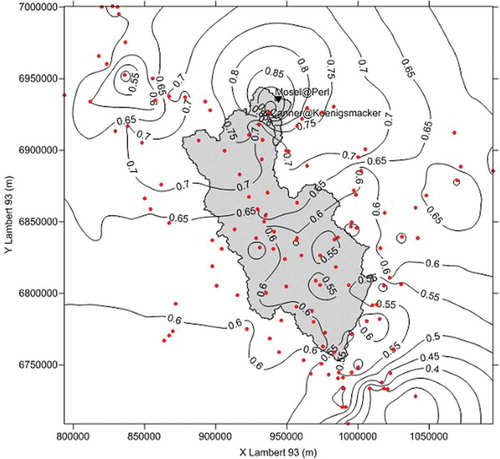
The results of cross-validation obtained for three representative streamgauges (Fig. 3(b)) show that fitted models produce quite good agreement between the estimated Pearson r values and the observed ones. It is therefore possible to assert that Pearson r values exhibit a spatial covariance structure. When used for mapping r values through ordinary kriging (Fig. 4), this spatial covariance generates a map correlation having a complex spatial structure. This map enables the most correlated streamgauges for a given location of interest to be identified (Fig. 4).

Fig. 4 Map showing the spatial distribution (ordinary kriging) of Pearson’s r values estimated between the daily streamflow time series at the Koenigsmacker streamgauge (Canner River) and all other streamgauges (•) in the study area. In the basic MC method, allowing only a single-best neighbour, the Koenigsmaker streamgauge would be used as a reference streamgauge for the Perl pollution-control site (▼) located on the Mosel River. Contours of the Canner@Koenigsmacker and Mosel@Perl catchments are also shown.

Concerning the benefit of a multiple neighbour configuration, Fig. 5 is convincing. An approach based on five neighbours allows a net gain of efficiency in comparison to a single-best neighbour approach for the tested period (from 0.429 to 0.590 for the mean efficiency and from 0.459 to 0.634 for the median efficiency). For 81% of the pollution-control sites, the selection of five neighbours leads to higher efficiency than using only the single-best neighbour, whereas this percentage is 62%, 57% and 47% when allowing five vs two, three and four neighbours, respectively. Selecting five neighbours also provides the smallest interdecile range and the highest 10% decile. Thus, we retained this neighbourhood as a reference for the application of the MC method.

Fig. 5 Changes in mean and percentiles (10% and 90%) for the performance of the MC method according to the number of neighbour catchments,for the 21 French pollution-control sites used (1990–2009).

SP method

We tested both options (model parameter averaging and model output averaging). The best efficiency according to the C2M_√Q criterion was obtained with the averaging option using the four closest donor catchments (Plasse et al. 2014). Oudin et al. (2008) obtained similar results on a larger set of French catchments.

DISP method

As the number of point flow measurements differs from one pollution-control site to another (see Table 2), we did not directly use the point flow measurements available for each site. Following Perrin et al. (2007), point flow values were randomly sampled from the daily observed hydrographs (Fig. 6). We tested different sizes of daily flow samples (n = 1, 2, 3, 5, 10, 30, 50, 200) in order to get an initial idea of the sensitivity of the DISP method to the density of the available hydrometric information. The same dates were sampled for the 142 donor catchments and the receiver catchment whose outlet is located close to pollution-control sites (Table 2).

Fig. 6 Example (of the Lauter@Wissembourg catchment) of random streamflow data sampling for selecting the neighbour catchments (DISP and Q–Q methods), n = 30 d. Dots (○) are used for computing the error metric defined in equation (3). Note that point flow measurements were stopped after 2002.

Since sampling was random for each value of n, we repeated it and computed the efficiency of the method 100 times, and took the mean C2M_√Q value to obtain more general results. The best efficiency was obtained with four donor catchments and a value of α  = 0, that is, when the only factor that influences the selection of the best donor catchments is the hydrological similarity with the location of interest (see equation (2)).

The efficiency of the method increases as the hydrometric information becomes denser at the location of interest. Plasse et al. (2014) have shown that this increase is significant up to n = 30 days.

Q–Q method

As for the implementation of the DISP method, we used random daily streamflow values for calculating the error metric (see equation (4)). The donor catchments were ranked according to their respective error calculated over the 100 replications of n.

The distributions of method efficiency show that higher efficiencies are obtained with multiple neighbour configurations (Fig. 7). The optimal efficiency level is reached with four neighbours.

Fig. 7 Impact of the size of daily flow samples (n) and the number of NCs on the efficiency of the Q–Q method. Results are given for the 21 French pollution-control sites used in this study and the period 1990–2009.

Moreover, we analysed the sensitivity of the Q–Q method efficiency to the size of daily flow samples. We successively tested values of 1, 5, 10, 20 and 50 days for n (Table 3). Results stabilize when n reaches 10 days. This indicates that optimal efficiencies are obtained for the Q–Q method as soon as a small number of point flow values (say 10) are used. Thus, in the framework of our comparative study, the Q–Q method is applied using four neighbours selected according to an error metric computed with n = 10 daily streamflow values.

Table 3 Impact of the number n of streamflow values sampled from the daily observed hydrographs on the efficiency (C2M_√Q) of the Q–Q method (option allowing four neighbours). Results are given for the 21 French pollution-control sites used in this study and the period 1990–2009.

Statistics	Number of streamflow values (n)*
	1	5	10	20	50
Minimum	0.340	0.354	0.435	0.435	0.435
Maximum	0.946	0.959	0.970	0.970	0.970
1st quartile (25%)	0.593	0.602	0.596	0.596	0.596
Median (50%)	0.717	0.767	0.766	0.766	0.766
3rd quartile (75%)	0.869	0.878	0.878	0.878	0.878
Mean	0.712	0.736	0.736	0.736	0.736

*sampling is repeated 100 times.

WHAT IS THE MOST EFFICIENT WAY TO PREDICT DAILY HYDROGRAPHS AT ALMOST UNGAUGED SITES?

Daily streamflow time series

Statistical distributions of efficiency values (Fig. 8) show that the SP, DISP and Q–Q methods are able to provide good fits for most of the observed daily hydrographs. Mean efficiency values are 0.619, 0.682 and 0.736, respectively. The mean efficiency is slightly poorer for the MC method, with a value of 0.590. The Q–Q method outperforms the other approaches and clearly appears as the best method for reconstructing daily streamflow time series when point flow measurements are available. Whatever the method, some daily hydrographs observed at the outlet of tested catchments are difficult to reproduce due to physical singularities (sandstone aquifers in the Ardennes and the northern part of the Vosges Massif; karstic influences in the upper part of the Meuse catchment).

Fig. 8 Comparison of efficiency for the four tested distance-based regionalization methods for the 21 French pollution-control sites used, 1990–2009. MC: map correlation method (option allowing five neighbours); SP: spatial proximity (output averaging); DISP: discrete parameterization of the GR4J rainfall–runoff model at the site of interest (option allowing four neighbours, n = 30 d, α = 0); Q–Q: streamflow–streamflow method (option allowing four neighbours, n = 10 d).

Flow types and pulse shape

Table 4 gives an example for the River Mosel at Perl of the number of days classified for different parts of the observed and simulated (with the Q–Q method) hydrographs. For both hydrographs, the number of days of falling limb is dominant (60%) compared with the two other phases, especially the recession one which is the less frequent (2%). Moreover, occurrences of rising limb and falling limb are underestimated by the Q–Q method, whereas the number of recession days is overestimated (220 days simulated vs 134 days observed).

Table 4 Contingency table of days classified for different parts of the hydrograph. Results are given for the daily observed and simulated (Q–Q method) hydrographs of the River Mosel at Perl (11522 km²) for the period 1990–2009. Q–Q: streamflow-streamflow method (option allowing four neighbours, n = 10 days).

	Simulated hydrograph				Total
	Days classified as…	Rising limb*	Falling limb	Recession (Baseflows)
	Rising limb*	2069	661	24	2754
Observed	Falling limb	636	3702	79	4417
hydrograph	Recession	6	11	117	134
	Total	2711	4374	220	7305

*including peak flows.

The most recurrent classification error occurs between rising limb days and falling limb days. This finding demonstrates the inability of the Q–Q method to properly reproduce pulse shape, leading to lag times between observed and simulated flood flows. Those facts can be generalized to other cross-validation sites, whatever the method of prediction.

As part of the assessment we computed, for each cross-validation site, the index of agreement with data of the contingency table diagonal (Fig. 9). Duration of the rising limb of the hydrograph is the most difficult to simulate (Fig. 9(a)). This shortcoming is not surprising since it is directly related to the non-linearity of the rainfall–runoff transformation, which hampers all prediction attempts whatever the prediction method. For the four tested methods, the best agreement was found for the falling limb whatever the cross-validation site (Fig. 9(b)). For the recession part, the agreement is very good for SP and DISP and poorer for the Q–Q and MC methods (Fig. 9(c)).

Fig. 9 Comparison of agreement for the four tested distance-based regionalization methods for the 21 French pollution-control sites used, 1990–2009: (a) rising limbs; (b) falling limbs; (c) recession (baseflows). See Fig. 8 for legend.

SPATIAL DISTRIBUTION OF NEIGHBOUR CATCHMENTS

Different distance-based regionalization schemes yield different collections of neighbour catchments (Fig. 10). The MC method is based on the selection of five neighbours identified as the best ones according to the correlation fields of donor catchments (Fig. 10(a)). As shown previously, this approach is generally less powerful.

Fig. 10 Maps showing the neighbour catchment(s) (in grey) for the target catchment of the Doller@Reiningue (▼), 187 km². (a) MC method; (b) SP method; (c) streamflow–streamflow method; and (d) DISP method. The four neighbours whose model parameters occur in more than half of the 100 simulations of n are indicated by white circles.

Note that the closest nested catchment is not always selected as a hydrological cousin of the receiver catchment, as shown by the application of the Q–Q method on a particular site of interest (see Fig. 10(b) vs Fig. 10(c)). Adjacent neighbours may be preferentially selected depending on the degree of hydraulic connectivity between the upstream/downstream streamgauge station and the target site.

The DISP approach makes it possible to draw multiple combinations of donor catchments from the regional library, which can be located far from the site of interest (Fig. 10(d)). This maximizes the probability of finding the best parameterization of the rainfall–runoff model at the location of interest through a library containing 142 × 4 model parameter vectors calibrated on real catchments.

IS A RANDOM DAILY STREAMFLOW SIMILAR TO A POINT FLOW MEASUREMENT?

This question raises the problem of the representativity of the streamflow measurement according to the time scale of the catchment response to the rainfall.

In this study, random daily streamflow values drawn from observed hydrographs were assumed to be similar to point flow measurements and used to optimally define the pool of donor catchments. In practice, the temporal extent of a streamflow measurement depends on the technique used (type of device, intrusive vs non intrusive techniques, etc.) and the size of the river gauging section. Except for very large and deep sections as, for example, the Amazon at Obidos, the measurement itself takes a short time (typically 1 hour). A point flow measurement is therefore representative of the mean hourly streamflow rather than a real mean value of streamflow at the daily time step. The realism of this assumption will depend on the type of catchment response (slow vs flashy) and on the flow conditions when the streamflow measurement is taken: during recession a point value is a good proxy for daily streamflow due to low water level variation in the gauging section. To check the realism of our assumption, we compared the point flow values drawn from the streamflow archive of the Rhine-Meuse French Water Agency to the daily values provided by the gauging station nearest to the pollution-control site. An example is given in Fig. 11 for two contrasting sized catchments having quite similar numbers of available point measurements.

Fig. 11 Comparison between point flow measurements and daily streamflow values. (a) Mosel@Sierck (pollution-control site) vs Mosel@Perl (streamgauge station): 270 days; the mean annual streamflow is close to 145 m³/s. (b) Meurthe@Fraize: 156 days; the mean annual streamflow is close to 2 m³/s. Measurement period refers to 1990–2005 in both cases.

As could be expected, some large differences occur especially in medium and high flows for both catchments whatever their size (Fig. 10(a) and (b)). This underlines the need to keep in mind what we expect from the regionalization method and to use the right field data for calibrating the regionalization methods. Hence, for a spatial generalization of streamflow simulation at a given time step using, for example, the DISP or the Q–Q method, it is recommended to obtain point flow measurements at the same time step.

DISCUSSION AND CONCLUSION

This study aims to evaluate the spatial generalization of four regionalization methods used in the reconstruction of daily hydrographs in a mesoscale area over two decades (1990–2009). The evaluation was based on a dense network of 149 donor catchments (≈1 streamgauge station per 250 km²) including nearby cross-validation sites of 21 almost ungauged control-pollution sites. In addition to the classical streamflow prognostic variable used in hydrology for assessment of regionalization methods, we used flow types and pulse shape (duration of rising limb and falling limb) as a timing qualitative indicator useful for meta-analysis of river water quality data.

A limited number of random point flow measurements, considered as historical and representative records of different flow conditions (low flows, floods, etc.), proved to be an efficient way to define a pool of behavioural neighbour catchments. As a result, the predictive uncertainty of regionalization methods accounting for scarce gauging data was significantly reduced in comparison to classical distance-based approaches (map correlation method and spatial proximity). Better insights of flow types and overall pulse shape are obtained. Rojas-Serna et al. (2006) as well as Montanari and Toth (2007) reached similar conclusions: hydrometric information may lead to a guided optimization of rainfall–runoff model parameters which, in turn, yields improved estimates of streamflow time series on almost ungauged catchments.

The implementation of the Q–Q method is simple and straightforward, since it requires only the definition of the transfer function of streamflow time series observed at the outlet of one or several neighbour catchment(s) to the target point. This definition should be seen as a learning process (Seibert and Beven 2009), as the optimal method parameterization is geographically and hydrologically specific. In terms of data requirement, only a few point flow measurements collected at the location of interest and representative of the prognostic hydrological variable are necessary. For the DISP approach, reliable rainfall and PET time series are needed in addition to continuous streamflow series for both donor and receiver catchments.

The application of the Q–Q method to our case study yields better results for assessing daily hydrographs using a multiple neighbour strategy in comparison to the single one. This is consistent with the results obtained by Andréassian et al. (2012) at the French national level by implementing a neighbour-catchment model calibrated on continuous streamflow time series and a larger catchments dataset.

The level of efficiency of the Q–Q method is likely to depend on the density of the donor catchments available for computing the method. We would expect that the supremacy of the Q–Q method over the other distance-based methods will fade when the number of potential hydrological neighbours decreases. To assess the impact of donor catchment density, we progressively reduced the density of the donor streamgauge network according to the distance to the target sites: for each of the 21 locations of interest, we calculated daily hydrographs over the 1990–2009 period according to the optimal version of the Q–Q method (i.e. four neighbours and n = 10 days), the only difference being that the four selected neighbours were drawn from networks progressively thinned by removing gauging stations located at a distance of less than 5, 10, 20, 30, 35 and 40 km from the location of interest. Figure 12 presents mean and percentiles of the efficiency for the Q–Q method in conjunction with the mean efficiencies obtained for the other methods for the full (i.e. existing) streamgauge network.

Fig. 12 Changes in mean and percentiles (10% and 90%) for the performance of the Q–Q method according to the reduction of the density of the donor streamgauge network for the 21 French pollution-control sites used, 1990–2009. Horizontal lines provide the mean efficiency of each of the three other regionalization methods considering the full (i.e. existing) donor streamgauge network, with the number of donor catchments for the current density level in parentheses. See Fig. 8 for legend.

It is interesting to note that (a) the gain of efficiency becomes negligible for a network density exceeding 30 stations per 10 000 km²; (b) the mean efficiency of the Q–Q method decreases slowly from the full (i.e. existing) donor streamgauge network (148 donor catchments; 39 stations per 10 000 km²) to a reduction by 40% of the streamgauge network (87 donor catchments; 23 stations per 10 000 km²); (c) at this density level, the mean efficiency of the Q–Q method reaches that of the DISP method; (d) below this value, the mean efficiency drops quickly; and (e) a similar mean efficiency between the Q–Q method and the MC method is obtained for a reduction of the network by almost 70%.

Thus, the Q–Q approach parameterized with a small set (e.g. 10) of discrete and contrasting daily flow data appears to be a robust and powerful method for interpolating daily hydrographs provided that neighbour(s) are not too far from the receiver catchment, i.e. the streamgauge network is sufficiently dense (at least 20 stations per 10 000 km²). In this case, and with the rainfall–runoff model tested, we come to the conclusion that hydrological neighbours are more informative than spatially transferred parameters. Considering these outcomes, we advocate that at-site monitoring of chemical and physical status of river water should additionally include a series of flow measurements made in different flow conditions, especially in data-scarce regions.

The issue of uncertainty has not been addressed explicitly in the framework of this paper; it was not within its scope. We presume that the neighbour catchment approach will be subject to less uncertainty than the rainfall–runoff modelling-based approach, as the only sources of uncertainty are the measurement error on observed flows and the error of the transfer function on reconstructed daily streamflows. This point should be confirmed by further investigations.

Funding

We would like to acknowledge the Rhine-Meuse French Water Agency for its financial support.

Acknowledgements

We would like to thank C. Conan for providing access to the point flow measurements database (SIERM database), Météo-France for providing the SAFRAN reanalysis data, the DREAL Lorraine through P. Battaglia for providing access to the HYDRO and the BAREME streamflow archives, the German Federal Waterways and Shipping Administration as well as the German Federal Institute of Hydrology (BfG) for providing the German streamflow data, and the Service public de Wallonie, Direction générale opérationnelle “Mobilité et Voies hydrauliques”, Direction de la Gestion hydrologique intégrée, Service d’Etudes Hydrologiques (SETHY) for making the Belgian streamflow data freely available. The authors gratefully acknowledge two anonymous reviewers for their suggestions which helped to make the paper more consistent and clear.

REFERENCES

- Andréassian, V., et al., 2012. Neighbours: nature’s own hydrological models. Journal of Hydrology, 414–415, 49–58. doi:10.1016/j.jhydrol.2011.10.007.
- Archfield, S.A. and Vogel, R.M., 2010. Map correlation method: selection of a reference streamgage to estimate daily streamflow at ungaged catchments. Water Resources Research, 46, W10513. doi:10.1029/2009WR008481.
- Blöschl, G.. 2005. Rainfall–runoff modelling of ungauged catchments. Article 133. In: M.G. Anderson, Managing ed. Encyclopaedia of hydrological sciences. Chichester: J. Wiley & Sons, 2061–2080.
- Burt, T.P., et al., 2010. Long-term monitoring of river water nitrate: how much data do we need? Journal of Environmental Monitoring, 12, 71–79. doi:10.1039/b913003a.
- Byrd, R.H., et al., 1995. A limited memory algorithm for bound constrained optimization. SIAM Journal on Scientific Computing, 16, 1190–1208. doi:10.1137/0916069.
- Chopart, S. and Sauquet, É., 2008. Usage des jaugeages volants en régionalisation des débits d’étiage (Using spot gauging data to interpolate low flow characteristics. Revue des Sciences de l’Eau/Journal of Water Science, 21 (3), 267–281. doi:10.7202/018775ar.
- Clausen, B., Pearson, C.P., and Downes, M.T., 1999. Relating potential denitrification rates to streamflow variability [online]. In: L. Heathwaite, ed. Impact of land-use change on nutrient loads from diffuse sources. Proceedings of IUGG 99 symposium HS3, Birmingham. Wallingford: International Association of Hydrological Sciences, IAHS Publ. 257, 127–134. Available from: http://iahs.info/uploads/dms/iahs_257_0127.pdf [Accessed 30 Aug 2014].
- Decloux, J.P. and Sary, M., 1991. Campagnes d‘étiage. Objectifs, traitement et valorisation des données (Low flows field campaigns. Objectives, data treatment and valorisation). Mosella, XXIII, 121–134.
- Drogue, G., et al., 2002. The applicability of a parsimonious model for local and regional prediction of runoff. Hydrological Sciences Journal, 47 (6), 905–920. doi:10.1080/02626660209492999.
- François, D. and Sary, M., 1990. Etude méthodologique des basses eaux. Estimation minimale des points de mesure (Methodological study of low flows. Estimation of minimal measurement points). Metz: CEGUM, Université de Metz.
- Guillaud, J.F. and Bourriel, L., 2007. Relationships between nitrate concentration and river flow, and temporal trends of nitrate in 25 rivers of Brittany (France). Revue des sciences de l‘eau/Journal of Water Science, 20 (2), 213–226.
- He, Y., Bárdossy, A., and Zehe, E., 2011. A review of regionalisation for continuous streamflow simulation. Hydrology and Earth System Sciences, 15, 3539–3553. doi:10.5194/hess-15-3539-2011.
- Hrachowitz, M., et al., 2013. A decade of Predictions in Ungauged Basins (PUB) – a review. Hydrological Sciences Journal, 58 (6), 1198–1255. doi:10.1080/02626667.2013.803183.
- Kay, A.L., et al., 2006. A comparison of three approaches to spatial generalization of rainfall–runoff models. Hydrological Processes, 20, 3953–3973. doi:10.1002/hyp.6550.
- Klemeš, V., 1986. Operational testing of hydrological simulation models. Hydrological Sciences Journal, 31 (1), 13–24. doi:10.1080/02626668609491024.
- Lang, C. and Gille, E. 2006. Une méthode d’analyse du tarissement des cours d’eau pour la prévision des débits d’étiage (A recession analysis method for low flow forecasting). Norois, 201 2006/4 [online]. Available from: http://norois.revues.org/1743; doi:10.4000/norois.1743 [Accessed 30 Aug 2014].
- Mathevet, T., et al., 2006. A bounded version of the Nash-Sutcliffe criterion for better model assessment on large sets of basins [online]. In: V. Andréassian, ed. Large sample basin experiments for hydrological model parameterisation: results of the Model Parameter Experiment—MOPEX. Wallingford, CT: International Association of Hydrological Sciences, IAHS Publ. 307, 211–219. Available from: http://iahs.info/uploads/dms/13614.21–211-219-41-MATHEVET.pdf [Accessed 19 Sep 2014].
- McIntyre, N., et al., 2005. Ensemble predictions of runoff in ungauged catchments. Water Resources Research, 41, W12434. doi:10.1029/2005WR004289.
- Montanari, A. and Toth, E., 2007. Calibration of hydrological models in the spectral domain: an opportunity for scarcely gauged basins? Water Resources Research, 43, doi:10.1029/2006WR005184.
- Oudin, L., et al., 2006. Dynamic averaging of rainfall–runoff model simulations from complementary model parameterizations. Water Resources Research, 42 (7), W07410. doi:10.1029/2005WR004636.
- Oudin, L., et al., 2008. Spatial proximity, physical similarity, regression and ungaged catchments: a comparison of regionalization approaches based on 913 French catchments. Water Resources Research, 44, W03413. doi:10.1029/2007WR006240.
- Pannatier, Y., 1996. VARIOWIN: software for spatial data analysis in 2D. New York: Springer-Verlag.
- Parajka, J., et al., 2013. Comparative assessment of predictions in ungauged basins—Part 1: runoff hydrograph studies. Hydrology and Earth System Sciences Discussions, 10, 375–409. doi:10.5194/hessd-10-375-2013.
- Perrin, C., et al., 2007. Impact of limited streamflow data on the efficiency and the parameters of rainfall—runoff models. Hydrological Sciences Journal, 52 (1), 131–151. doi:10.1623/hysj.52.1.131.
- Perrin, C., et al., 2008. Discrete parameterization of hydrological models: evaluating the use of parameter sets libraries over 900 catchments. Water Resources Research, 44, W08447. doi:10.1029/2007WR006579.
- Perrin, C., Michel, C., and Andréassian, V., 2003. Improvement of a parsimonious model for streamflow simulation. Journal of Hydrology, 279, 275–289. doi:10.1016/S0022-1694(03)00225-7.
- Plasse, J., et al., 2014. Apport des jaugeages ponctuels à la reconstitution des chroniques de débits moyens journaliers par simulation pluie-débit: l’exemple du bassin Rhin-Meuse. (Using point flow measurements for guided reconstruction of daily streamflow time series through continuous flow simulation: a regional case study on the Rhine-Meuse district). La Houille Blanche-Revue Internationale de l’Eau, 1, 45–52. doi:10.1051/lhb/2014007.
- Quintana-Seguí, P., et al., 2008. Analysis of near surface atmospheric variables: validation of the SAFRAN analysis over France. Journal of Applied Meteorology and Climatology, 47, 92–107. doi:10.1175/2007JAMC1636.1.
- Rojas-Serna, C., et al., (submitted). How should a rainfall–runoff model be parameterized in an almost ungauged catchment? A methodology tested on 705 catchments. Water Resources Research.
- Rojas-Serna, C., et al., 2006. Ungauged catchments: how to make the most of a few streamflow measurements? [online]. In: V. Andréassian, ed. Large sample basin experiments for hydrological model parameterisation: results of the Model Parameter Experiment—MOPEX. Wallingford, CT: International Association of Hydrological Sciences, IAHS Publ. 307, 230–236. Available from: http://iahs.info/uploads/dms/13616.23-230-236-43-ROJAS-SERNA.pdf [Accessed 30 August 2014].
- Seibert, J. and Beven, K., 2009. Gauging the ungauged basin: how many discharge measurements are needed? Hydrology and Earth System Sciences, 13, 883–892. doi:10.5194/hess-13-883-2009.
- Woods, R. and Sivapalan, M., 1999. A synthesis of space-time variability in storm response: rainfall, runoff generation, and routing. Water Resources Research, 35 (8), 2469–2485. doi:10.1029/1999WR900014.