Potential of the LASH model for water resources management in data-scarce basins: a case study of the Fragata River basin, southern Brazil

ABSTRACT

The objective of this study was to evaluate, based on a data-scarce basin in southern Brazil, the potential of the Lavras Simulation of Hydrology (LASH) model for estimating daily streamflows, annual streamflow indicators and the flow–duration curve. It was also used to simulate the different runoff components and their consistency with the basin physiographical characteristics. The statistical measures indicated that LASH can be considered suitable according to widely used classifications and when compared with other studies involving hydrological models. LASH also showed satisfactory results for annual indicators, especially for maximum and average annual streamflows, as well as for the flow–duration curve. It was found that the model was consistent with the basin characteristics when simulating runoff components. The results obtained in this study allowed us to conclude that the LASH model has the potential to aid practitioners in water resources management of basins with scarce data and similar soil and land-use conditions.

Editor A. Castellarin; Associate editor Y. Gyasi-Agyei

KEYWORDS:

• Lavras Simulation of Hydrology
• hydrology
• hydrograph
• flow–duration curve
• annual streamflow indicators
• subtropical climate

1 Introduction

Hydrological models are being used increasingly as tools for decision making in management of water resources. They use a complex system of equations, usually aided by computer processing, such as a geographical information system (GIS) (Jain et al. 2004, Soulis and Dercas 2007, Efstratiadis et al. 2008, Beskow et al. 2011a, 2011b). The main objective of a hydrological model is to quantitatively describe the components of the hydrological cycle in a given basin. There are many applications of hydrological models for basins, such as real-time flood forecasting, flood frequency estimation, hydraulic structure design (spillways, dams, bridges, etc.), derivation of flow–duration curves, climate and land-use change impact assessment, and integrated basin management (Mosley and McKerchar 1993, Pilgrim and Cordery 1993, Wheater 2008, Vivoni et al. 2011).

Hydrological basin models require input data on both the temporal and the spatial scale. However, these data are often difficult and expensive to obtain and may exert influence on the performance of models with respect to simulation of hydrological processes. Database requirements are quite variable among models and this can be a limitation in applying a model to a given basin. In this context, there are some hydrological models that have intense database requirements, such as the Soil and Water Assessment Tool (SWAT) (Arnold et al. 1998), the Water Erosion Prediction Project (WEPP) (Flanagan and Nearing 1995), and the Limburg Soil Erosion Model (LISEM) (De Roo and Jetten 1999). Regardless of the conceptual hydrological model used, White and Chaubey (2005) state that sensitivity, calibration and validation steps must be followed to assess whether the model will be able to give reliable results for water resources management in the region of interest.

In most developing countries, such as Brazil, there is a shortage of public hydrological information, at the basin scale, to be used for water resources management. The hydrological monitoring that has been conducted in Brazil predominantly focuses on larger basins, typically for electric power generation purposes (Beskow et al. 2009). Additionally, experimental basins have been monitored by educational and private institutions for specific purposes, but the information is not readily available. This is a limiting factor in Brazil for the application of complex or simplified hydrological models.

To overcome these limitations, hydrological models have been developed such that their formulations require a smaller amount of information that is readily available, thereby minimizing its acquisition cost. Among them, the Lavras Simulation of Hydrology (LASH) model (Viola 2008, Beskow 2009) has aroused interest in the scientific community. This model employs a simplified hydrological formulation and was developed to estimate the main components of the hydrological cycle in basins, especially those in developing countries where databases are usually limited.

This model has been successfully applied in basins in southeastern and northern regions of Brazil, as reported by Mello et al. (2008), Viola et al. (2009, 2013, 2014a, 2014b) and Beskow et al. (2011a, 2011b, 2013). However, the LASH model has not had its performance evaluated under different basin conditions in southern Brazil.

As Brazil is a continental country, there is great heterogeneity in the physiographical and climatic characteristics of its regions. The LASH model has been applied particularly to basins located in southeastern Brazil, which have specific soil and climate characteristics. Thus, it is necessary to evaluate the performance of the LASH model for basin conditions with physiographical characteristics distinct from those already studied with the LASH model.

The Fragata River basin (FRB) is strategic for the economic and social development of the southern State of Rio Grande do Sul (RS). It is worth noting that its main river is an important tributary of the São Gonçalo channel, which supplies drinkable water for the population of Rio Grande–RS (197 228 inhabitants) and is also an important waterway that connects the Patos Lagoon to the Mirim Lagoon. The latter is a transboundary lagoon and it shares its water body between Brazil and Uruguay.

The FRB has historically suffered the impact of human activities and experienced situations of water erosion and floods, such as the extreme rainfall event that occurred in January 2009. This event had over 500 mm of rainfall during less than 12 h (Bainy and Teixeira 2012), thereby causing economic and social losses, especially in the peri-urban zone of Pelotas city (328 275 inhabitants) near the basin outlet.

Despite the aforementioned importance, no studies have been carried out in the FRB regarding the application of hydrological models to assess appropriate tools for estimation of streamflow on a daily scale, droughts and floods, and simulation of alterations in hydrological behaviour due to climate and land-use changes, among other applications. In this context, the objective of this study was to evaluate whether the LASH model, which requires a smaller amount of information, has the ability to estimate daily streamflow, floods and droughts in the Fragata River basin drainage area upstream from the Passo dos Carros outlet, as well as to adequately estimate the different components of runoff in this basin.

2 Material and methods

2.1 LASH model

The Lavras Simulation of Hydrology (LASH) model, in its first version, is a continuous hydrological simulation model classified as deterministic and with a semi-conceptual basis, which simulates the following components in daily time increments: actual evapotranspiration, interception of rainfall by land cover, capillary rise, soil water storage, direct surface runoff, subsurface flows and baseflows. This model is based on other models, notably the SCS-CN modified by Mishra et al. (2006) to estimate the direct surface runoff (“overland flow”), the equation of Brooks and Corey (Rawls 1993) to estimate both subsurface flows and baseflows, and the Muskingum-Cunge linear model for drainage network routing described in Tucci (2005). The LASH model takes into consideration the spatial and temporal variability of all input variables used in the hydrological components, since the basin is divided into cells of uniform size.

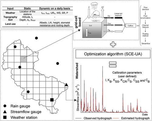
The LASH model is a continuation of the model developed by Mello et al. (2008). The main difference is that LASH uses a distributed rather than a lumped or semi-distributed formulation, and has a computationally efficient algorithm to execute autocalibration of the most sensitive parameters for the basin of interest. The hydrological modelling in LASH has three basic modules, as illustrated in Figure 1 (Beskow et al. 2011a). As the model employs a distributed approach, the first module includes the calculation of each component of the water balance in each basin grid cell, in which it is possible to estimate direct surface runoff, and subsurface flows and baseflows. The second module is intended to consider the lag effect in the reservoirs, which is simulated in the model by the concept of simple linear reservoirs, as described by Collischonn (2001). The third module, in turn, performs the streamflow routing in the drainage network by the Muskingum-Cunge linear method as described by Tucci (2005).

Figure 1. Modelling steps in the LASH hydrological model for its grid-cell-based version, where P is the rainfall, ET is the actual evapotranspiration, D_CR is the capillary rise, D_S is the direct surface runoff, D_SS is the subsurface flow, and D_B is the baseflow.

The LASH model (Mello et al. 2008, Viola 2008, Beskow 2009; Beskow et al. 2011b) was developed in the Delphi programming language (Windows environment) and provides a graphical user interface. This interface allows users to import maps from different geographical information systems (GIS), facilitating its use.

The unknown parameters, or those indirectly measurable on the basin scale, are calibrated in the LASH model by a built-in optimization routine based on the shuffled complex evolution algorithm (SCE-UA [University of Arizona]) (Duan et al. 1992). This global parameter optimization technique executes the hydrological simulation routine, compiling a soil, land-use and weather spatial and temporal database until it converges to an appropriate set of values representing the basin. This version of the model considers a single value for each calibration parameter. It would not be feasible to calibrate a model in which each grid cell had a value for each calibration parameter. The development team has worked hard to make available the second version of the model, which considers spatial discretization by sub-basins and allows users to calibrate parameters for each sub-basin, soil type or land-use class.

The input maps used by the LASH model are derived from the digital elevation model (DEM), with land-use, soil-type and drainage network maps. All the input parameters (relief, vegetation and soil parameters) can be spatially distributed. In addition, the model’s spatial structure allows the water balance to be executed in each grid cell and at each time step; in other words, each hydrological process (e.g. runoff components, interception, evapotranspiration, etc.) is determined through a given variable, taking into account its spatial and temporal variability. In addition to these maps, the LASH model also needs two other files (tables) in a spreadsheet format. The first table has to contain observed streamflow records (m³ s⁻¹) as well as information on meteorological variables. The optimization method in LASH uses the observed hydrograph to seek appropriate parameters for the basin of interest such that the simulated hydrograph is close to that observed, and this task is accomplished by minimizing or maximizing a given objective function (root mean square error, Nash-Sutcliffe coefficient, etc.). In the second table, users have to store information on the temporal variation of the land-use parameters (leaf area index, vegetation height, albedo, surface resistance and root system depth).

More details on the LASH hydrological model can be found in Mello et al. (2008), Beskow et al. (2011a, 2011b) and Viola et al. (2013).

2.2 The analysed basin and database

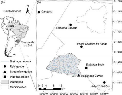
The Fragata River basin (FRB) was chosen in this study to evaluate the LASH hydrological model under representative conditions in southern Brazil. This choice was due to the economic and social importance that the FRB has for the southern Rio Grande do Sul region. In addition, this basin has soil classes under different land-use conditions compared to all the basins already evaluated using the LASH model (Mello et al. 2008, Viola et al. 2009, 2013, 2014a, 2014b, Beskow et al. 2011a, 2011b, 2013). Considering the availability of hydrological monitoring, under the responsibility of the Brazilian National Water Agency (ANA), the drainage area upstream from the Passo dos Carros outlet (FRB-PC) was selected, totalling an area of approximately 132 km² (Fig. 2).

Figure 2. (a) Location of the Fragata River basin; (b) drainage area upstream from the Passo dos Carros outlet and the monitoring network used.

Taking the Pelotas agro-meteorological station located in the county of Capão do Leão–RS as representative of the FRB-PC, the climatological series from 1971 to 2000 indicated that the average annual temperature in this region was 17.8°C, ranging from −3°C (minimum temperature) to 39.6°C (maximum temperature), the average annual relative humidity was 80.7%, ranging over 78.6–83.3%, the average annual wind speed was 3.5 m s⁻¹, ranging over 2.6–4.0 m s⁻¹ and the average annual potential evapotranspiration was 1103.1 mm, ranging over 985.8–1568.7 mm. The average annual rainfall, considering the same climatological normal period, was 1366.9 mm; however, values between 823.2 mm and 1893.2 mm were recorded in the 1971–2000 period (Empresa Brasileira de Pesquisa Agropecuária [Embrapa n.d.]). According to the Köppen climate classification, the climate of the FRB-PC region is characterized as Cfa (Kuinchtner and Buriol 2001), indicating a wet subtropical climate with an average temperature for the hottest month of over 22°C.

Figure 2(b) also illustrates the monitoring network employed in this study, notably: (a) the Passo dos Carros outlet, which provided a historical series of daily average streamflows obtained from the Brazilian National Water Agency (ANA); (b) the raingauges at Canguçu and Ponte Cordeiro de Farias (whose datasets were also acquired from ANA), INMET Pelotas (under the responsibility of the Brazilian National Institute of Meteorology), and Embrapa Cascata (for which the Brazilian Agricultural Research Company, Embrapa, is responsible), which provided total daily rainfall series; and (c) the weather station Embrapa Sede (Embrapa Clima Temperado), which provided series of rainfall, air temperature, relative humidity, wind speed and number of sunshine hours on a daily scale.

Among the historical data series used, some have been registered since the 1960s; however, due to lack-of-data problems and series collected for differing periods, the 1994–2008 period was chosen for hydrological modelling. The year 1994 was used for model warm-up, while the period from 1995 to 2000 was applied for calibration, and the period 2001–2008 for validation of the LASH model. It should be mentioned that it is necessary to have minimally basic meteorological and rainfall–runoff datasets for the basin of interest in order to evaluate a hydrological model similar to the one under study. Therefore, these aspects do not make the model more or less demanding in terms of historical series.

The information on relief was extracted from the cartographic database developed by Hasenack and Weber (2010), which includes the entire database of the State of Rio Grande do Sul at a 1:50 000 scale, providing contour lines, points of known altitude and vectored hydrography. These information layers were used as input in the GIS environment ArcGIS (ESRI 2014), with the objective of developing a hydrologically consistent digital elevation model (HCDEM), which is the basic input information for hydrological modelling using the LASH model. According to the HCDEM for the FRB- PC, the altitude varies between 20 m and 347.9 m, with an average value of 113.8 m, while the slope of the basin varies between 0% and 177%, with an average of 14.2%.

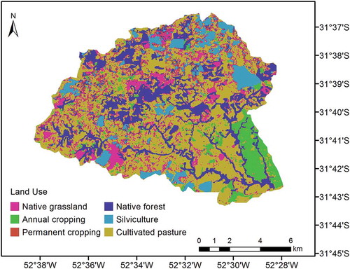
The parameters related to vegetation (height, root system depth, leaf area index, albedo and stomatal resistance) can be derived from (i) an existing land-use map or a satellite image interpretation, in conjunction with a literature review for determination of these parameters by land-use class; or (ii) determination of the aforementioned parameters under field conditions and integration with a land-use map. With regard to the land-use map for the FRB-PC, Landsat satellite images acquired from the website of the Brazilian Institute for Space Research (INPE) were used to derive the map. Scenes 221_81 and 222_82 were used in the interpretation of the images with the aid of Environment for Visualizing Images (ENVI) software following the suggestions of Perrota (2005). The land-use map was based on interpretation of these satellite images using a maximum-likelihood supervised classification method, in conjunction with 100 training samples obtained in the FRB-PC with a portable GPS. These samples allowed both the identification of the main land uses in the FRB-PC and the development of its land-use map, which presented the following percentage distributions (Fig. 3): native grassland (4.5%), annual cropping (6.5%), permanent cropping (0.4%), native forest (20.6%), silviculture (9.0%) and cultivated pasture (59.0%). From Figure 3 and a literature review, the values of land-use-related parameters, shown in Table 1, were adopted as input parameters for the LASH hydrological model.

Table 1. Parameter values associated with land-use classes identified in the FRB-PC for hydrological modelling with LASH.

Land-use classes	LAI* (m^2 m^−2)	Height (m)	Albedo	Surface resistance (s m^−1)	Root system depth (mm)
Silviculture	3.5^(a)	5^(f)	0.3–0.18^(g)	100^(h)	1500^(i)
Permanent cropping	1.82–3.62^(b)	1.13–1.62^(b)	0.15–0.2^(h)	40^(f)	500^(j)
Native grassland	0.5	0.2	0.20–0.26^(h)	70^(f)	500^(k)
Annual cropping	0.17–6.02^(c)	0–1.52^(c)	0.15–0.20^(h)	40^(f)	500^(j)
Native forest	6.25^(d)	10^(f)	0.13–0.18^(g)	100^(h)	2000^(i)
Cultivated pasture	1.86–3.99^(e)	0.5^(f)	0.20–0.26^(h)	70^(f)	600^(j)

*LAI: Leaf Area Index; ^aAlmeida and Soares (2003), ^bFavarin et al. (2002), ^cManfron et al. (2003), ^dMarques Filho et al. (2005), ^eFagundes et al. (2006), ^fCollischonn (2001), ^gMiranda et al. (1996), ^hShuttleworth (1993), ⁱLima (1996), ^jAllen et al. (1998), ^kViola (2008).

Figure 3. Land-use map for the FRB-PC.

The parameters associated with soils (depth and soil water contents at saturation and permanent wilting point) can be derived from: (i) a soil map combined with a literature review seeking to characterize these three parameters by soil class; (ii) a soil map combined with a soil survey seeking to characterize these parameters by soil class; or (iii) a soil survey for mapping the spatial distribution of each parameter. The soil classification map was obtained from the soil survey conducted by Brasil (1973). However, in this study only the drainage area encompassed by the FRB-PC’s boundaries was considered (Fig. 4). From the information in Figure 4 and the classification recommended by Soil Survey Staff (2010), the percentage distributions of the main soil types in the FRB-PC are Paleudult (34.2%), Hapludalf + Udorthent (56.7%) and Albaqualf (9.1%).

Figure 4. Main soil types in the FRB-PC and the 15 km spatial transect established for soil sampling.

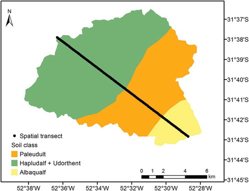
The strategy adopted regarding soil information in the LASH model was to quantify soil attributes at 100 points equidistantly spaced along a 15 km spatial transect in the FRB-PC (Fig. 4). Disturbed and undisturbed soil samples were collected at each point in order to determine soil bulk density, soil texture (clay, sand and silt fractions), saturated soil hydraulic conductivity and soil water retention curves according to the methodologies described in Embrapa (1997). From each soil water retention curve, values of soil water content at saturation (θ_S) and at the permanent wilting point (θ_PWP) were adopted as those relating to water content retained at tensions of 0 kPa and 1500 kPa, respectively (Reichardt and Timm 2012). From the soil map (Fig. 4) and the distribution of soil properties along the spatial transect, representative values were established for each soil type (Table 2).

Table 2. Values of soil properties associated with land-use classes identified in the FRB-PC for hydrological modelling with LASH.

Soil classes	Saturated soil water content θS (cm^3 cm^−3)*	Soil water content retained at permanent wilting point θPWP (cm^3 cm^−3)**	Soil depth Z (mm)***
Paleudult	0.456	0.195	1500
Hapludalf + Udorthent	0.447	0.185	1000
Albaqualf	0.405	0.168	500

*Saturated soil water content; **Soil water content retained at permanent wilting point; ***Soil depth.

Using the soil survey published in Brasil (1973), it was also possible to obtain the soil depth values (Z) for each soil class. The water balance control layer was based on the crop root depths identified in the FRB-PC (Table 1). However, in areas where the root system of the existing crop was deeper than Z, the latter value (Table 2) was employed, as recommended by Collischonn (2001).

The data requirements of the LASH are lower than those of other models such as SWAT, WEPP and LISEM, especially because of parameters related to soil and vegetation. The model parametrization and the number of soil-related and vegetation-related attributes make the LASH model suitable for data-scarce basins.

2.3 Performance analysis of the model

To verify the accuracy of the results generated by the LASH model in the calibration and validation steps, the following statistical measures were calculated: Nash-Sutcliffe coefficient, C_NS (Nash and Sutcliffe 1970) (Equation (1)) and its logarithmic version, C_NS log(Q) (Equation (2)), and the estimated streamflow relative error, ∆Q (Equation (3)):

(1)

(2)

(3)

where is the streamflow observed at time t (m³ s⁻¹), is the streamflow estimated at time t by the LASH model (m³ s⁻¹), is the average observed streamflow (m³ s⁻¹), is the logarithm of the streamflow observed at time t (m³ s⁻¹), is the logarithm of the streamflow estimated at time t (m³ s⁻¹) and is the average logarithm of the observed streamflow (m³ s⁻¹).

The C_NS and C_NSlog(Q) values can range from –∞ to 1. Moriasi et al. (2007) suggested the following classification for C_NS values with respect to the performance of a hydrological model, considering the daily time interval: C_NS > 0.65, very good fit; 0.54 < C_NS < 0.65, good fit; and 0.50 < C_NS < 0.54, satisfactory fit. According to Zappa (2002), hydrological models can be used for simulation when C_NS > 0.5. The same classification was used as reference for C_NSlog(Q) values. The ΔQ measure allows us to infer whether the model over- or underestimated the streamflow values (Liew et al. 2007, Andrade et al. 2013). Liew et al. (2007) suggested the following classification for ΔQ expressed in terms of its absolute value: |ΔQ| < 10%, very good fit; 10% < |ΔQ| < 15%, good fit; 15% < |ΔQ| < 25%, satisfactory fit; and |ΔQ| ≥ 25%, unsatisfactory fit.

In addition, the LASH model also had its accuracy verified in the FRB-PC to estimate annual minimum, average and maximum streamflows, flow–duration curves, and the different streamflow components.

3 Results and discussion

Table 3 contains the lower and upper bounds of the calibration parameters as suggested by Beskow et al. (2011b) for the optimization algorithm known as shuffled complex evolution (SCE/UA; Duan et al. 1992). This table also provides the calibrated values of the following parameters for the FRB-PC: initial abstraction coefficient (λ), hydraulic conductivity of the shallow saturated zone reservoir (K_B), hydraulic conductivity of the subsurface reservoir (K_SS), maximum flow returning to soil by capillary rise (K_CR), surface reservoir response time parameter (C_S), subsurface reservoir response time parameter (C_SS), and baseflow recession time parameter (C_B). Even though the LASH model can be used with six calibration parameters, the authors opted to use seven parameters in this study. Depending on the hydrological model and its set-up, more than 10 or 20 parameters must be calibrated. As in any other model for long-term simulation that depends on rainfall and streamflow series, the calibration process may take some minutes or hours due to the length of the time series. In this context, it was found that the model application did not require extensive calibration.

Table 3. Lower and upper bounds used for each parameter calibrated by the LASH model and the respective optimized values for the FRB-PC.

Parameter	Description	Lower and upper bounds	FRB-PC
λ	Initial abstraction coefficient (dimensionless)	0–0.5	0.147
KB	Shallow saturated zone reservoir hydraulic conductivity (mm d^−1)	0–6	0.192
KSS	Subsurface reservoir hydraulic conductivity (mm d^−1)	0–250	2.08
KCR	Maximum flow returning to soil by capillary rise (mm d^−1)	0–5	2.67
CS	Surface reservoir response time parameter (dimensionless)	–	3 389.2
CSS	Subsurface reservoir response time parameter (dimensionless)	–	28 216.4
CB	Baseflow recession time (d)	–	49.9

The calibrated value of λ for the FRB-PC was 0.147. By applying the modified curve number method (CN-MMS; Mishra et al. 2003) for isolated analysis of direct surface runoff in basins, Mishra et al. (2006) and Beskow et al. (2009) found that this parameter can vary considerably depending on the basin under study. Mishra et al. (2006) obtained λ values between 0 and 0.21 for various basins in the United States, with drainage areas ranging from 0.17 to 74 ha, while Beskow et al. (2009) found a mean value of λ = 0.133 when considering the soil depth as constant, and of λ = 0.063 for variable soil depths for a 4.7 km² basin in the state of Minas Gerais, Brazil.

When considering the value for λ in the LASH model calibration, in which other hydrological processes are addressed, and using the CN-MMS method to estimate direct surface runoff, some studies in Brazil should be highlighted: (a) Mello et al. (2008) found λ values ranging from 0.001 to 0.5 (in several sub-basins) for a 2080 km² sub-basin of the Rio Grande basin (Southeast region); (b) Viola et al. (2009) obtained λ values from 0.01 to 0.2 for the Aiuruoca River basin (2094 km²), also in the Southeast; and (c) Beskow et al. (2011b) obtained λ equal to 0.136 for a 32 km² basin in Minas Gerais State. Mishra et al. (2006), Mello et al. (2008), Beskow et al. (2009), Beskow et al. (2011a, 2011b) and Viola et al. (2014a) suggested that this parameter should be calibrated instead of using a fixed value (λ = 0.2), as suggested when used for the SCS-CN method (SCS 1972).

According to Mishra et al. (2003), the variation in λ values could be attributed to the alteration of some factors, such as the different climatic characteristics and rainfall patterns of the study area, which might have influenced the initial soil moisture conditions. This parameter is directly related to initial abstractions, i.e. water losses that occur before the generation of direct surface runoff, such that the lower the λ for the same rainfall event, the lower the amount of water lost before yielding effective rainfall. Therefore, the soil type also has great influence on the generation of direct surface runoff as well as on the characteristic value of λ in a basin.

The calibration procedure in LASH resulted in K_B and K_SS values of 0.192 mm d⁻¹ and 2.08 mm d⁻¹, respectively, for the FRB-PC (Table 3). Viola et al. (2009) found K_B values of 0.1–2.5 mm d⁻¹ and K_SS values of 0.01–82.65 mm d⁻¹ for the Aiuruoca River basin using a semi-distributed version (for sub-basins) of the LASH model. This version was also used by Mello et al. (2008) for the Grande River basin, where calibration culminated in a K_B value of 0.9 mm d⁻¹ and K_SS values of 12–182.4 mm d⁻¹. Using the distributed version of the LASH model in a 32 km² basin in southeastern Brazil, Beskow et al. (2011b) found a K_B value of 3.18 mm d⁻¹ and a K_SS value of 182.15 mm d⁻¹.

Because the K_B and K_SS parameters are closely associated with soil type, changes in their values are expected in different basins. The FRB-PC has shallow soils, poorly developed (Albaqualf), with the presence of restrictive layers regarding drainage (Hapludalf + Udorthent and Paleudult). The differences between K_B and K_SS values obtained by Beskow et al. (2011b) and those obtained in the present study can be attributed to the low values of the saturated soil hydraulic conductivity (K_SAT) obtained in this study. Alvarenga et al. (2011) obtained K_SAT values of 61.25–145.83 mm h⁻¹ in the basin evaluated by Beskow et al. (2011b).

Considering the K_SAT values determined along the 15 km spatial transect and the distribution of the percentage areas of the main soil classes in the FRB-PC (Fig. 4), the average K_SAT value was 24.17 mm h⁻¹ in this study. Based on the classification of K_SAT values proposed by Pruski et al. (1997) for Brazilian soils aimed at applications of the curve number method (SCS 1972), the K_SAT value in the FRB-PC can be considered to have the potential to generate direct surface runoff greater than average. In studies using the LASH model carried out by Mello et al. (2008) and Viola et al. (2009), the soil class Cambisols was the most common in the basins, where K_B and K_SS values were lower than those obtained by Beskow et al. (2011b). The values of K_B and K_SS obtained in the present study are consistent with the main soil classes in the FRB-PC (Fig. 4), especially when compared to other studies using the same model in Brazil.

The C_B parameter is related to the groundwater reservoir’s lag time and plays an important role in the characterization of baseflow in basins. This parameter can be either calibrated in the LASH model or derived for a specific basin from its hydrograph considering a typical recession period, as suggested by Viola (2008). However, it is known that there may be a variation in this parameter when analysing different recession periods in the same hydrograph. In the studies conducted by Beskow et al. (2011b) and Viola et al. (2013) using the LASH model, C_B was obtained directly from the observed hydrographs following the recommendations of Viola (2008). The LASH model resulted in a calibrated value of 49.9 d in the FRB-PC (Table 3). Analysing the most evident recession period in the FRB-PC outlet, which occurred from 18 May to 16 June 1996, the calculated C_B was approximately 35 d. Since the calculated value of C_B strongly depends on the experience of the hydrologist regarding the choice of the recession period, the uncertainties in its estimation can be minimized through the calibration procedure. Therefore, it is recommended to calibrate the C_B parameter in other studies involving the LASH model, especially in basins where the baseflow contribution is significant.

The historical series of streamflows monitored at the FRB-PC outlet and the corresponding series estimated by the LASH model, considering the periods of calibration and validation separately, are illustrated in Figure 5.

Figure 5. Hydrographs monitored in the FRB-PC and hydrographs estimated by the LASH model in the same basin for calibration (a) and validation (b) periods.

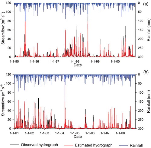
One can infer from Figure 5 that the LASH model was able to capture the overall behaviour of the observed hydrograph in the FRB-PC for the studied period. In order to make it easier to quantitatively evaluate the model performance, the results of the statistical measures applied in this study are presented in Table 4.

Table 4. Statistical measures to assess the performance of the LASH model in the calibration and validation steps for the FRB-PC.

Statistical measure	Calibration	Validation
Nash-Sutcliffe coefficient (CNS)	0.805	0.719
Logarithm of the Nash-Sutcliffe coefficient (log CNS)	0.693	0.830
Estimated streamflow relative error (∆Q)	−0.011	0.025

The C_NS values for the FRB-PC were 0.805 and 0.719 for the calibration and validation periods, respectively (Table 4). According to the classification proposed by Moriasi et al. (2007), the fit can be considered “very good” for the calibration and validation periods in the FRB-PC. Additionally, according to the classification indicated by Zappa (2002), LASH can be used for hydrological modelling in the FRB-PC since the C_NS values were greater than 0.5.

Considering the log version of the C_NS (Table 4) as a statistical measure for LASH performance evaluation, values of 0.693 and 0.830 were obtained for the calibration and validation periods, respectively. Thus, the model fit is classified as “very good” for the calibration and validation periods according to the classification of Moriasi et al. (2007). When the criterion of Zappa (2002) is applied, the LASH model can be used for hydrological modelling in the FRB-PC since the log values (C_NS) were greater than 0.5. The C_NS values, when used in its logarithmic form, are strongly influenced by the hydrograph recessions. Therefore, based on the performance achieved by the aforementioned statistical measure, it is clear that the LASH model was able to adequately capture the streamflow behaviour on the daily scale during drought periods. In this context, it can be inferred that the model has the potential to be applied to estimate minimum streamflow in the FRB-PC, which is fundamental for water resources management in this region.

The estimated streamflow relative error values (ΔQ) (Table 4) indicate the model’s tendency to over- or underestimate observed streamflow values (Yapo et al. 1996). A ∆Q value equal to zero indicates an ideal estimation of the streamflow by the model, while positive values indicate an overestimation and negative ones indicate an underestimation. On average, the streamflows were underestimated by 1.1% in the calibration period for the FRB-PC, while in the validation period, on average, the streamflows were overestimated by 2.5%. Based on the ΔQ classification proposed by Liew et al. (2007), the fit of the LASH model for the FRB-PC can be considered “very good”, since |ΔQ| < 10%. The results for ΔQ reinforce the potential of applying the LASH hydrological model to estimate streamflows on a daily basis in the basin under study.

The statistical measures used to evaluate the performance of the LASH hydrological model for the FRB-PC indicate that the model produced promising results for this basin, strengthening the potential of LASH already proven in southeastern Brazil (Mello et al. 2008, Viola et al. 2009, 2013, 2014a, 2014b, Beskow et al. 2011a, 2011b, 2013).

On analysing Figure 5, one can verify that the model under- and overestimated some streamflow peaks during the calibration and validation steps. Although this aspect is unwanted, this behaviour has been commonly observed in hydrological model applications, and can be attributed to model formulation and datasets used (Mello et al. 2008). In analysing hydrographs from several different hydrological models, difficulties have been observed in the estimation of streamflow peaks (Green et al. 2006, Bormann et al. 2007, Notter et al. 2007, Stackelberg et al. 2007, Thanapakpawin et al. 2007, Gomes et al. 2008, Viola et al. 2009, 2014a, Beskow et al. 2011a, 2011b, 2013). Viola et al. (2009) mentioned that hydrological models usually have limitations in estimating streamflow peaks, especially those related to the representation of the rainfall spatial variability and to the time step adopted in the modelling. Green et al. (2006) reported some aspects that can influence streamflow peak estimation: (i) representativeness of the stage-discharge rating curve; (ii) the existing monitoring network; and (iii) the distribution of rainfall gauge stations in the study area.

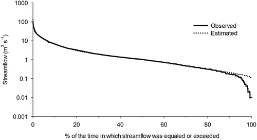
In order to complement the analysis of the LASH model performance in the FRB-PC, Figure 6 depicts observed and estimated minimum, mean and maximum annual streamflows, while Figure 7 shows the observed flow–duration curve and that estimated by the LASH model.

Figure 6. Values observed in the FRB-PC, and those estimated by the LASH model for minimum annual streamflow (a), mean annual streamflow (b), and maximum annual streamflow (c).

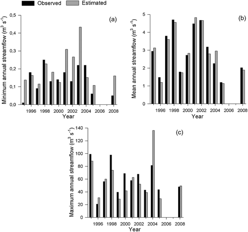
Figure 7. Observed flow–duration curve and curve estimated by the LASH model in the FRB-PC.

In the context of annual indicators of streamflow, the LASH model presented satisfactory results, especially for mean annual streamflow (Fig. 6(b)) and maximum annual streamflow (Fig. 6(c)). In basins with quite different physiographical characteristics when compared to the FRB-PC, Viola et al. (2009, 2013) and Beskow et al. (2013) also verified the good performance of the LASH model in estimating minimum, mean and maximum annual streamflows.

Although it is known that estimation of maximum streamflows by hydrological models is complex, reliability in estimating this indicator is crucial for many practical purposes, serving as a basis for hydraulic projects, soil conservation systems in basins, and basin flood management. The estimation of maximum streamflows through a conceptual model such as LASH can be a good option, thus serving as an additional alternative to the traditional techniques of transformation of heavy rainfall into streamflow, as reported by Beskow et al. (2015) and Caldeira et al. (2015). Information on minimum streamflows enables practitioners to design pumping systems for irrigation, identify drought susceptibility in a given basin, and determine streamflows for water rights. The importance of mean streamflow characterization lies in water resources management, because this variable is an indicator commonly used to estimate water yield of a basin, thus allowing definition of both water availability and potential for streamflow regulation in reservoirs.

The flow–duration curve is a hydrological function, represented by a graph, that has extreme importance in the management of water resources as it allows one to estimate streamflow indicators associated with different exceedence frequencies, thereby having numerous practical applications, as reported by Booker and Snelder (2012), Guo and Quader (2009) and Li et al. (2010). Figure 7 shows that the flow–duration curve estimated by the LASH model is similar to that observed in the FRB-PC during the period under consideration, especially for exceedence frequencies (durations) between 0 and 95%, and this interval is considered the most important for water resources management. Considering durations of 10, 20, 30, 40, 50, 60, 70, 80 and 90%, the values for the ∆Q statistical measure were −2.3, −6.6, −1.4, 3.6, −2.3, −0.4, −3.0, −3.5 and 22.5%, respectively, indicating a “very good” estimate for the considered durations, except for 90%, which was deemed “satisfactory”, according to the ΔQ classification proposed by Liew et al. (2007). The LASH hydrological model has been successfully evaluated in southeastern Brazil with respect to its accuracy in generating flow–duration curves (Viola et al. 2009, 2013, Beskow et al. 2013).

The conceptual formulation of the LASH model combined with the promising results of this study and those already presented by Viola et al. (2009, 2013) and Beskow et al. (2013) reinforce its potential for estimating flow–duration curves in Brazilian basins with both different physiographical characteristics and limited databases. Therefore, LASH can be used in place of, or to complement, hydrological regionalization techniques applied to the derivation of flow–duration curves (Li et al. 2010, Mamum et al. 2010, Booker and Snelder 2012), and low streamflows, such as Q₉₀ and Q₉₅ (Laaha and Blöschl 2005, 2006, Castiglioni et al. 2009, Vezza et al. 2010, Beskow et al. 2014).

It is of great importance that a hydrological model has adequate performance, taking into account appropriate statistical measures, such as those discussed above, since the model must provide reliability regarding its results from the basin point of view. However, the capabilities of the model in estimating and understanding the behaviour of the different runoff components in the basin of interest are as important as its acceptable overall performance in terms of statistical measures (Beskow et al. 2011b). Figure 8 shows the quantitative importance of each runoff component estimated by the LASH model for the FRB-PC for the 1995–2008 period.

Figure 8. Percentage breakdown of each runoff component considering the hydrograph estimated by the LASH model from 1995 to 2008 in the FRB-PC.

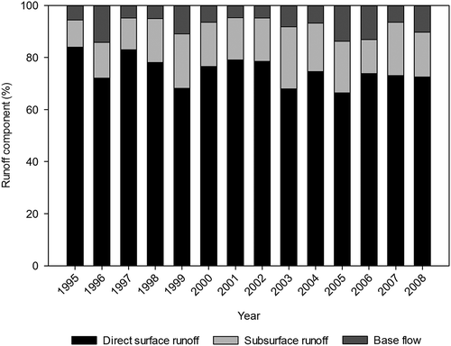
The predominance of direct surface runoff in the FRB-PC is evident in comparison with the two other runoff components (Fig. 8). Considering the 1995–2008 period, the direct surface runoff, subsurface flow and baseflow components corresponded, on average, to 74.9, 16.9 and 8.2% of the total runoff, respectively. According to the average annual rainfall values calculated from the gauging stations used in this study, a direct relationship was found between the percentages of the different runoff components and the average annual rainfall in the basin. The average annual rainfall in the FRB-PC ranged from 1008.1 mm to 2008.8 mm, whereas amplitudes of 66.4–84%, 10.4–23.9% and 4.7–14.2% were obtained by the LASH model for the direct surface runoff, subsurface flow and baseflow, respectively.

The predominance of direct surface runoff in this basin may be associated with both the dominant land use in the FRB-PC, that is, cultivated pasture in approximately 59% of the area (Fig. 3), corroborating the findings of Viola et al. (2013), and low groundwater recharge, thus supporting the results highlighted in this study. It is important to point out the significant estimated portion of subsurface runoff in the FRB-PC (10.4–23.9%). According to Beskow et al. (2011b), subsurface runoff can be insignificant in many basins, but it can be critical when evaluating forested basins or headwater basins. The results for this runoff component in the FRB-PC corroborate the findings of Beskow et al. (2011b), since the basin area is approximately 30% forested (Fig. 3). The results of this study with respect to the percentage of each runoff component are in contrast to those found by Beskow et al. (2011b) and Viola et al. (2013), also applying the LASH hydrological model. These researchers found greater importance in the baseflow component, which could be attributed to the types of soil and land-use classes in the studied basins. The results found in the FRB-PC using the LASH model, along with those obtained in other regions of Brazil, reinforce the necessity and importance of application and analysis of this model in different physiographical and climatic regions of the country.

4 Conclusions

Based on the results presented and discussed, it can be concluded that:

1. the hydrological behaviour of the Fragata River basin (FRB-PC) was represented adequately by the LASH hydrological model for the estimation of the hydrograph on a daily basis, and also for the estimation of maximum, minimum and mean streamflows, and the flow–duration curve;

2. the different components of the total runoff were estimated by the LASH model, accordingly, considering the soils types and land uses in the FRB-PC;

3. the LASH model requires a small amount of input information, which, combined with its promising results, allows us to consider LASH to be a tool with potential applications in southern Brazil aimed at water management.

Disclosure statement

No potential conflict of interest was reported by the authors.

Additional information

Funding

The authors wish to thank CNPq for financial support of this research and scholarships to the first, second and fifth authors, and FAPERGS for financial support of this research and a scholarship to the fourth author.

References

- Allen, R.G., et al. 1998. Crop evapotranspiration: guidelines for computing crop water requirements (Irrigation and Drainage Paper). Roma: FAO.
- Almeida, A.C. and Soares, J.V., 2003, Comparação entre uso de água em plantações de eucalipto grandis e floresta ombrófila densa (mata Atlântica) na costa leste do Brasil. Revista Árvore, 27 (2), 159–170. doi:10.1590/S0100-67622003000200006
- Alvarenga, C.C., et al. 2011. Continuidade espacial da condutividade hidráulica saturada do solo na bacia hidrográfica do Alto Rio Grande, MG. Revista Brasileira De Ciência Do Solo, 35 (5), 1745–1757. doi:10.1590/S0100-06832011000500029
- Andrade, M.A., et al. 2013. Simulação hidrológica em uma bacia hidrográfica representativa dos Latossolos na região Alto Rio Grande, MG. Revista Brasileira De Engenharia Agrícola E Ambiental, 17 (1), 69–76. doi:10.1590/S1415-43662013000100010
- Arnold, J.G., et al. 1998. Large area hydrologic modeling and assessment: part I: model development. Journal of the American Water Resources Association, 34 (1), 73–89. doi:10.1111/j.1752-1688.1998.tb05961.x
- Bainy, B.K. and Teixeira, M.S., 2012. Evaluation of the model MM5 performance in an extreme precipitation event and a deeper analysis of its meteorological causes. In: 26th Conference on Severe Local Storms, 5–8 November 2012, Nashville, TN, EUA.
- Beskow, S., 2009. LASH Model: a hydrological simulation tool in GIS framework. Thesis (PhD). Federal University of Lavras.
- Beskow, S., et al. 2009. Estimativa do escoamento superficial em uma bacia hidrográfica com base em modelagem dinâmica e distribuída. Revista Brasileira de Ciência Do Solo, 33 (1), 169–178. doi:10.1590/S0100-06832009000100018
- Beskow, S., et al., 2011a. Development, sensitivity and uncertainty analysis of LASH model. Scientia Agricola, 68 (3), 265–274.
- Beskow, S., et al. 2011b. Performance of a distributed semi-conceptual hydrological model under tropical watershed conditions. Catena, 86 (3), 160–171. doi:10.1016/j.catena.2011.03.010
- Beskow, S., et al. 2013. Hydrological prediction in a tropical watershed dominated by oxisols using a distributed hydrological model. Water Resources Management, 27 (2), 341–363. doi:10.1007/s11269-012-0189-8
- Beskow, S., et al. 2014. Índices de sazonalidade para regionalização hidrológica de vazões de estiagem no Rio Grande do Sul. Revista Brasileira de Engenharia Agrícola e Ambiental, 18 (7), 740–746. doi:10.1590/S1415-43662014000700012
- Beskow, S., et al., 2015. Multiparameter probability distributions for heavy rainfall modeling in extreme Southern Brazil. Journal of Hydrology: Regional Studies, 4 (B), 123–133.
- Booker, D.J. and Snelder, T.H., 2012. Comparing methods for estimating flow duration curves at ungauged sites. Journal of Hydrology, 434–435, 78–94. doi:10.1016/j.jhydrol.2012.02.031
- Bormann, H., et al. 2007. Analyzing the effects of soil properties changes associated with land use changes on the simulated water balance: a comparison of three hydrological catchment models for scenario analysis. Ecological Modelling, 209 (1), 29–40. doi:10.1590/S0100-204X2002000600005
- Brasil, 1973. Levantamento de reconhecimento dos solos do Estado do Rio Grande do Sul. Recife: Ministério da Agricultura-Departamento Nacional de Pesquisa Agropecuária/Divisão de Pesquisa Pedológica.
- Caldeira, T.L., et al. 2015. Modelagem probabilística de eventos de precipitação extrema no estado do Rio Grande do Sul. Revista Brasileira de Engenharia Agrícola e Ambiental, 19 (3), 197–203. doi:10.1590/1807-1929/agriambi.v19n3p197-203
- Castiglioni, S., et al. 2009. Prediction of low-flow indices in ungauged basins through physiographical space-based interpolation. Journal of Hydrology, 378 (3–4), 272–280. doi:10.1016/j.jhydrol.2009.09.032
- Collischonn, W., 2001. Simulação hidrológica de grandes bacias. Thesis (PhD). Federal University of Rio Grande do Sul.
- De Roo, A.P.J. and Jetten, V.G., 1999, Calibrating and validating the LISEM model for two data sets from the Netherlands and South Africa. Catena, 37 (3–4), 477–493. doi:10.1016/S0341-8162(99)00034-X
- Duan, Q., Sorooshian, S., and Gupta, V., 1992, Effective and efficient global optimization for conceptual rainfall-runoff models. Water Resources Research, 28 (4), 1015–1031. doi:10.1029/91WR02985
- Efstratiadis, A., et al. 2008. HYDROGEIOS: A semi-distributed GIS-based hydrological model for modified river basins. Hydrology and Earth System Sciences, 12 (4), 989–1006. doi:10.5194/hess-12-989-2008
- Embrapa (n.d.) Estação Agroclimatológica de Pelotas, Convênio Embrapa/UFPEL. Available from: http://www.cpact.embrapa.br/agromet/estacao/estacao.html [Accessed 19 March 2015].
- Embrapa, (1997). Manual de métodos de análise de solos. 2nd ed. Rio de janeiro: Embrapa Solos.
- Environmental Systems Research Institute (ESRI), 2014. Redands, CA, 265p.
- Fagundes, J.L., et al. 2006. Características morfogênicas e estruturais do capim-braquiária em pastagem adubada com nitrogênio avaliadas nas quatro estações do ano. Revista Brasileira de Zootecnia, 35 (1), 21–29. doi:10.1590/S1516-35982006000100003
- Favarin, J.L., et al. 2002. Equações para a estimativa do índice de área foliar do cafeeiro. Pesquisa Agropecuária Brasileira, 37 (6), 769–773. doi:10.1590/S0100-204X2002000600005
- Flanagan, D.C. and Nearing, M.A., 1995. USDA-water erosion prediction project (WEPP) hillslope profile and watershed model documentation. West Lafayette: National Soil Erosion Research Laboratory.
- Gomes, N.M., et al. 2008. Aplicabilidade do LISEM (Limburg Soil Erosion Model) para simulação hidrológica em uma bacia hidrográfica tropical. Revista Brasileira de Ciência do Solo, 32 (6), 2483–2492. doi:10.1590/S0100-06832008000600025
- Green, C.H., et al. 2006. Hydrologic evaluation of the soil and water assessment tool for a large tile-drained watershed in Iowa. Transactions of the ASABE, 49 (2), 413–422. doi:10.13031/2013.20415
- Guo, Y. and Quader, A., 2009, Derived flow–duration relationships for surface runoff dominated small urban streams. Journal of Hydrologic Engineering, 14 (1), 42–52. doi:10.1061/(ASCE)1084-0699(2009)14:1(42)
- Hasenack, H. and Weber, E., 2010. Base cartográfica vetorial continua do Rio Grande do Sul – escala 1:50.000. [DVD-ROM]. Porto Alegre: UFRGS-IB-Centro de Ecologia.
- Jain, M.K., et al. 2004. A GIS based distributed rainfall-runoff model. Journal of Hydrology, 299 (1–2), 107–135. doi:10.1016/j.jhydrol.2004.04.024
- Kuinchtner, A. and Buriol, G.A., 2001, Clima do estado do Rio Grande do Sul segundo a classificação climática de Köppen e Thornthwaite. Disciplinarum Scientia, 2 (1), 171–182.
- Laaha, G. and Blöschl, G., 2005, Low flow estimates from short stream flow records—a comparison of methods. Journal of Hydrology, 306 (1–4), 264–286. doi:10.1016/j.jhydrol.2004.09.012
- Laaha, G. and Blöschl, G., 2006, A comparison of low flow regionalisation methods—catchment grouping. Journal of Hydrology, 323 (1–4), 193–214. doi:10.1016/j.jhydrol.2005.09.001
- Li, M., et al. 2010. A new regionalization approach and its application to predict flow duration curve in ungauged basins. Journal of Hydrology, 389 (1–2), 137–145. doi:10.1016/j.jhydrol.2010.05.039
- Liew, M.W., et al. 2007. Suitability of SWAT for the conservation effects assessment project: A comparison on USDA - ARS watersheds. Journal of Hydrologic Engineering, 12 (2), 173–189. doi:10.1061/(ASCE)1084-0699(2007)12:2(173)
- Lima, W.P., 1996. Impacto ambiental do eucalipto. 2nd ed. Piracicaba: EDUSP.
- Mamum, A.A., et al. 2010. Regionalisation of low flow frequency curves for the Peninsular Malaysia regionalisation of low flow frequency curves for the Peninsular Malaysia. Journal of Hydrology, 381 (1–2), 174–180. doi:10.1016/j.jhydrol.2009.11.039
- Manfron, P.A., et al., 2003. Modelo do índice de área foliar da cultura do milho. Revista Brasileira de Agrometeorologia, 11 (2), 333–342.
- Marques Filho, A.O., Dallarosa, R.G., and Pachêco, V.B., 2005, Radiação solar e distribuição vertical de área foliar em floresta: reserva biológica do Cuieiras, ZF2. Acta Amazônica, 35 (4), 427–436. doi:10.1590/S0044-59672005000400007
- Mello, C.R., et al. 2008. Development and application of a simple hydrologic model simulation for a Brazilian headwater basin. Catena, 75 (3), 235–247. doi:10.1016/j.catena.2008.07.002
- Miranda, A.C., et al., 1996. Carbon dioxide fluxes over a cerrado sensu stricto in central Brazil. In: J.H.C. Gash, et al., eds. Amazonian deforestation and climate. New York: Wiley, 353–364.
- Mishra, S.K., et al. 2003. A modified SCS-CN method: characterization and testing. Water Resources Management, 17 (1), 37–68. doi:10.1023/A:1023099005944
- Mishra, S.K., et al. 2006. An improved Ia-S relation incorporating antecedent moisture in SCS-CN methodology. Water Resources Management, 20 (5), 643–660. doi:10.1007/s11269-005-9000-4
- Moriasi, D.N., et al. 2007. Model evaluation guidelines for systematic quantification of accuracy in watershed simulations. Transactions of the ASABE, 50 (3), 885–900. doi:10.13031/2013.23153
- Mosley, M.P. and McKerchar, A.I., 1993. Streamflow. In: D. Maidment, ed. Handbook of hydrology. New York: McGraw-Hill, 8.1–8.39.
- Nash, J.E. and Sutcliffe, J.V., 1970, River flow forecasting through conceptual models part I — A discussion of principles. Journal of Hydrology, 10 (3), 282–290. doi:10.1016/0022-1694(70)90255-6
- Notter, B., et al., 2007. Impacts of environmental change on water resources in the Mt. Kenya Region. Journal of Hydrology, 343 (3–4), 266–278.
- Perrotta, M.M., 2005. Processamento digital básico de imagens de sensores remotos ópticos para uso em mapeamento geológico – programa ENVI. Belo Horizonte: CPRM.
- Pilgrim, D.H. and Cordery, I., 1993. Flood runoff. In: D. Maidment, ed. Handbook of hydrology. New York: McGraw-Hill, 9.1–9.42.
- Pruski, F.F., et al. 1997. Model to design level terraces. Journal of Irrigation and Drainage Engineering, 123 (1), 8–12. doi:10.1061/(ASCE)0733-9437(1997)123:1(8)
- Rawls, W.J. 1993. Infiltration and soil water movement. In: D. Maidment, et al. ed. Handbook of hydrology. New York: McGraw-Hill, 1–51.
- Reichardt, K. and Timm, L.C., 2012. Solo, planta e atmosfera: conceitos, processos e aplicações. 2nd ed. Barueri: Manole.
- SCS, 1972. Section 4: hydrology. In: Soil Conservation Service/USDA, ed. National engineering handbook. Washington: USDA Soil Conservation Service.
- Shuttleworth, W.J., 1993. Evaporation. In: D. Maidment, ed. Handbook of hydrology. New York: McGraw-Hill, 4.1–4.53.
- Soil Survey Staff, 2010. Keys to soil taxonomy. 11th ed. Washington: USDA-Natural Resources Conservation Service. http://www.nrcs.usda.gov/wps/portal/nrcs/detail/soils/survey/class/taxonomy/?cid=nrcs142p2_053580
- Soulis, K. and Dercas, N., 2007, Development of a GIS-based spatially distributed continuous hydrological model and its first application. Water International, 32 (1), 177–192. doi:10.1080/02508060708691974
- Stackelberg, N.O., et al. 2007. Simulation of the hydrologic effects of afforestation in the Tacuarembó River Basin, Uruguay. Transactions of the ASABE, 50 (3), 455–468. doi:10.13031/2013.22636
- Thanapakpawin, P., et al. 2007. Effects of land use change on the hydrologic regime of the Mae Chaem river basin, NW Thailand. Journal of Hydrology, 334 (1–2), 215–230. doi:10.1016/j.jhydrol.2006.10.012
- Tucci, C.E.M., 2005. Modelos hidrológicos. Porto Alegre: UFRGS/ABRH.
- Vezza, P., et al., 2010. Low flows regionalization in North-Western Italy. Water Resources Management, 24, 4049–4074. doi:10.1007/s11269-010-9647-3
- Viola, M.R., 2008. Simulação hidrológica na região Alto Rio Grande à montante do Reservatório de Camargos/CEMIG. Thesis (Master’s Degree). Federal University of Lavras.
- Viola, M.R., et al. 2009. Modelagem hidrológica na bacia hidrográfica do rio Aiuruoca, MG. Revista Brasileira de Engenharia Agrícola e Ambiental, 13 (5), 581–590. doi:10.1590/S1415-43662009000500011
- Viola, M.R., et al. 2013. Applicability of the LASH model for hydrological simulation of the Grande river basin, Brazil. Journal of Hydrologic Engineering, 18 (12), 1639–1652. doi:10.1061/(ASCE)HE.1943-5584.0000735
- Viola, M.R., et al. 2014a. Impacts of land-use changes on the hydrology of the Grande river basin headwaters, Southeastern Brazil. Water Resources Management, 28 (13), 4537–4550. doi:10.1007/s11269-014-0749-1
- Viola, M.R., et al. 2014b. Assessing climate change impacts on Upper Grande River Basin hydrology, Southeast Brazil. International Journal of Climatology, 35 (6), 1054–1068. doi:10.1002/joc.4038
- Vivoni, E.R., et al. 2011. Real-world hydrologic assessment of a fully-distributed hydrological model in a parallel computing environment. Journal of Hydrology, 409 (1–2), 483–496. doi:10.1016/j.jhydrol.2011.08.053
- Wheater, H.S., 2008. Modeling hydrological processes in arid and semi-arid areas: an introduction to the workshop. In: H.S. Wheater, S. Sorooshian, and K.D. Sharma, eds. Hydrological modeling in arid and semi-arid areas. New York: Cambridge University, 1–20.
- White, K.L. and Chaubey, I., 2005, Sensitivity analysis, calibration, and validations for a multisite and multivariable SWAT model. Journal of the American Water Resources Association, 41 (5), 1077–1089. doi:10.1111/jawr.2005.41.issue-5
- Yapo, P.O., et al. 1996. Automatic calibration of conceptual rainfall-runoff models: sensitivity to calibration data. Journal of Hydrology, 181 (1–4), 23–48. doi:10.1016/0022-1694(95)02918-4
- Zappa, M., 2002. Multiple-response verification of a distributed hydrological model at different spatial scales. Thesis (PhD). Swiss Federal Institute of Technology.