Improving rainfall–runoff modelling through the control of uncertainties under increasing climate variability in the Ouémé River basin (Benin, West Africa)

ABSTRACT

The objective of this paper is to understand how the natural dynamics of a time-varying catchment, i.e. the rainfall pattern, transforms the random component of rainfall and how this transformation influences the river discharge. To this end, this paper develops a rainfall–runoff modelling approach that aims to capture the multiple sources and types of uncertainty in a single framework. The main assumption is that hydrological systems are nonlinear dynamical systems which can be described by stochastic differential equations (SDE). The dynamics of the system is based on the least action principle (LAP) as derived from Noether’s theorem. The inflow process is considered as a sum of deterministic and random components. Using data from the Ouémé River basin (Benin, West Africa), the basic properties for the random component are considered and the triple relationship between the structure of the inflowing rainfall, the corresponding SDE that describes the river basin and the associated Fokker-Planck equations (FPE) is analysed.

EDITOR D. Koutsoyiannis; ASSOCIATE EDITOR D. Gerten

KEYWORDS:

• Fokker-Planck equation (FPE)
• least action principle (LAP)
• probability distribution
• river basin
• stochastic differential equation (SDE)
• system dynamics
• uncertainty

1 Introduction

Recent decades have witnessed increasing concern among the international scientific community about climate change and its impacts on the hydrological cycle (van Dam 1999). Today, there is much evidence that the planet is warming up, largely as a result of human generated greenhouse gases (Kundzewicz et al. 2014, IPCC 2014a, b). Therefore, managing water resources is more challenging than ever, largely due to the risks associated with multiple types of uncertainty (both aleatory and epistemic; Khatri 2013). Since the 1970s, sub-Saharan Africa, and in particular West Africa, is facing water-related uncertainties posed by the pressures of global change. A shortage in rainfall ranging from 20% to 30% has been observed throughout the region, leading to a decrease in river flows ranging from 40% to 60% (Afouda et al. 2007). Nowadays, floods and flash floods occur more frequently with greater and greater intensity and have become one of the most devastating natural hazards in West Africa. In 2009 severe flooding was observed in Burkina Faso and Mali; in 2010 flood disaster affected more than 680 000 people and caused the deaths of 46 people in Benin (World Bank 2011). In 2012, “killer floods” inducing more than 50 fatalities each occurred in Niger and Nigeria (Kundzewicz et al. 2014).

To efficiently adapt to these extreme events and climate change in general, it is important to consider preventive actions. Flood prevention and, more generally, water resources management planning rely on an understanding of the water cycle in West Africa. For the purpose of planning, one usually assumes that hydrological processes in a particular river basin can be described by probability distributions that are not changing over time (Strupczewski and Mitosek 1995). However, the more that extreme events happen due to climate change and unpredictable human activities, the less historical characteristics of these processes can be assumed essentially constant over time, and the more challenging it is to plan for integrated water resources management (IWRM) and adaptation policy. Thus, extrapolation using historical data is no longer valid for these events that increase uncertainty about the future. The key question that arises is how best to include these non-stationarity considerations in water planning and management (Hanggi and Ljung 1995, Alamou 2011). Strupczewski and Mitosek (1995) proposed improving the existing statistical procedures based on a probability distribution by allowing its parameters to vary in time. They concluded, however, that in the non-stationary case, this approach increases the error of quantile estimation and that this error increases with extrapolation time length. A promising approach is to take advantage of the optimality principle embodied in the least action principle (LAP), as explained by Noether’s theorem, to minimize uncertainties in modelling hydrological systems and from deficiency in our knowledge. This will be beneficial for predicting the impact of different forms of uncertainty on the overall water availability, in a single framework, for water users and decision makers.

Therefore, the objective of this paper is to understand how the natural dynamics of a time-varying catchment transforms the random component of rainfall and how this transformation influences the river discharge. To this end, this paper develops a rainfall–runoff modelling approach that aims to capture the multiple sources and types of uncertainty in a single framework. The main assumption is that hydrological systems are nonlinear dynamical systems which can be described by stochastic differential equations (SDE). Such equations arise when the elements which give rise to the representations of continuous deterministic dynamical system in the form of ordinary differential equations (ODE) are considered subject to environmental fluctuations or noise. The SDE theory is well developed and has found wide applications in most branches of sciences, including hydrology and water resources engineering (Bodo et al. 1987, Mtundu and Koch 1987, Serrano and Unny 1987, Cushman 1987, Konecny and Nachtnebel 1995, Hanggi and Ljung 1995, Alamou 2011). In this paper, the dynamics of the system are based on the LAP designed to minimize uncertainties related to rainfall – runoff transformation processes and scaling law (physical models).

The uncertainties addressed in this study come from three important aspects: uncertainties linked to the model structure and the model parameters, uncertainties linked to the correlation between input and output of the model, and uncertainties linked to the random component of rainfall. Using data from the Ouémé River basin (Benin, West Africa), the properties of the random component of rainfall are investigated. It is argued that the white noise process and the associated Brownian motion are acceptable approximations to the random component of rainfall over the Ouémé River basin. The triple relationship between the structure of the rainfall process, the corresponding stochastic differential equation that describes the river basin, and the associated Fokker-Planck equations (FPE) are analysed. The time-dependent probability distribution for the resulting discharge is obtained in the form of fundamental and approximate solutions of the FPE. A comparison is made between the derived time-dependent probability distributions and an empirical probability distribution of the outflow.

2 Methodology

The inflow process representing all irregular variations of hydro-meteorological processes is considered as a sum of deterministic and random components that embraces data uncertainties (e.g. measurement) and sample uncertainties (e.g. number of data) (Konecny and Nachtnebel 1995). Hence, the deterministic hydrological model based on the least action principle (HyMoLAP) is fed by a stochastic input. The main advantage of an SDE is that it provides a physically transparent and mathematically tractable description of the stochastic dynamics of a temporally varying catchment and can significantly improve the estimation of uncertainty. As noted by Koutsoyiannis (2013), changes in hydrological systems occur on all time scales, from minute to geological, but our limited senses and life span as well as the short time window of instrumental observations restricts our perception to the most apparent daily to yearly variations. However, we herein restrict our view to those short-term noises superimposed on the daily cycle, having in mind that the processes associated with hydrological systems are usually more complex. The driving process of an SDE plays a key role in the dynamics and future evolution of that SDE. Our approach will be especially effective if the noise that describes the random component of rainfall can be represented as the time derivative (in the sense of a generalized function) of a stationary process with independent increments on non-overlapping intervals. In that case, the solution of the SDE is a Markov process whose properties are well known (Denisov et al. 2009, Alamou 2011).

2.1 Model description

The hydrological model based on the least action principle (HyMoLAP) is described by:

(1)

(2)

where Z describes the variation of the initial state of the catchment, ψ describes the model input, Y describes the model structure, λ and μ are the physical parameters of the model, and Q stands for the river discharge.

Equation (1) describes explicitly the production process (i.e. the action of the unsaturated zone that accounts for evaporation and evapotranspiration and divides the resulting rainfall event into two components: overland and underground) and Equation (2) describes the transformation process (i.e. the process by which the rainfall volumes for the overland component and the underground component are transformed into runoff). Here, Equations (1) and (2) form the basic ODE describing the deterministic dynamics of the system (Biao et al. 2015). The HyMoLAP model has been used successfully in rainfall–runoff modelling for the Bétérou and Save catchments of the Ouémé River (Afouda and Alamou 2010, Alamou 2011, Biao et al. 2015). The choice of this model is determined by the purposes targeted. By coupling two classical theories we wish to take advantage of the optimizing properties embodied in the physics-based deterministic HyMoLAP and the statistical consistency of the Ito SDE.

2.2 Uncertainty management with HyMoLAP

In the majority of cases, hydrological systems can be described by a deterministic model, but this kind of model does not represent the system in a truly ideal way. In a hydrological system, as in almost all other natural systems, fluctuations are present and are caused by the chaotic nature of the system. As a consequence, these fluctuations do not allow for purely deterministic descriptions. For this reason, the stochastic formulation of HyMoLAP is derived from its foundation in the SDE, which has already been applied successfully in a wide range of hydrological applications.

In practice, knowledge of the functions and that describe, respectively, the model input and the model structure is subject to different types of uncertainty: one class of uncertainty is related to our imperfect knowledge of the physical phenomenon and another class of uncertainty is related to the quantitative evaluation of the parameters of the environment (especially rainfall). These forms of uncertainty can therefore be included in the structure of the model. To this end, the functions and can be viewed as the sum of the mean and a stochastic noise term. The deterministic Equations (1) and (2) are transformed into an SDE. This SDE allows us to derive the evolution of the total variance of river discharge.

The random functions and can be written in the form:

(3)

(4)

where and are, respectively, the means of and ; and stand, respectively, for the standard deviations of and .

It is appropriate to model the stochastic parts as a Gaussian white noise process with zero mean and delta correlated structure, described by:

(5)

Here, is the variance of the Gaussian white noise process, is the Dirac delta function, describes mathematical expectation.

The Gaussian white noise is not Riemann-integrable. However, it can be described as the formal derivative in time of a Wiener process, i.e.

Thus, the stochastic formulation of Equations (1) and (2) reads:

(6)

(7)

The system Equations (6) and (7) can then be written in vector form (Afouda et al. 2004, Alamou 2011):

(8)

One can, without loss of generality, write , and the following vector notations can be derived:

The solution of the SDE (Equation (8)) is a Markov diffusion process. Subsequently, U(t)is fully determined if the joint probability density function of the random variable U(t) is defined for all finite sets of t. This is, however, a very ambitious goal, which is difficult to achieve in most cases. In practice, it is satisfactory if a limited number of moments of the solution process are derived. This can be achieved by the method of moment equations, which relies on deriving effective equations for the statistical moments.

We now concentrate on the output as derived from the scalar form of Equation (8), dQ(t) = f(Q,t)dt + G(Q,t)dW(t). Following Ito’s lemma (an identity used in Ito calculus to find the differential of a time-dependent function of a stochastic process), if ϕ(Q,t) is a real scalar function of the solution process that is continuously differentiable in time t and that has continuous second partial derivative with respect to Q, then the stochastic differential of ϕ can be written as follows:

(9)

Taking expectation on both sides of Equation (9) yields

(10)

since

Now, if , is the nth moment, equations for the moments can be defined as follows:

(11)

From Equation (11) the low-order moments (mean and variance) of the output discharge can be evaluated with HyMoLAP. Thus, the equation of the first moment can be obtained from Equation (11) by setting :

(12)

where denotes the mathematical expectation.

The second moment can be derived in the same way by taking :

(13)

Equation (12) can be combined with Equation (13) to get the evolution of the variance in the form:

(14)

Equations (12) and (14) give, respectively, the evolution of the mean and the evolution of the spread around the mean. These equations can be used in the process of decision making for planning purposes. Equation (14) exhibits the structure of uncertainty. The total variance of the output is shown explicitly to have three components. The first component on the right hand side of Equation (14) is equivalent to the usual results given by standard statistical theory; the second and third terms are specific to the SDE properties. The second term reflects the influence of the dynamical structure of the model and the third term is explicitly part of the variance due to the choice of random noise. Therefore, it can be concluded that not only the choice of model for the dynamical structure of the river basin is important, but also investigation of the stochastic properties of the random component of rainfall must be carefully carried out.

3 Application to the Ouémé River basin at Bonou

3.1 Study area

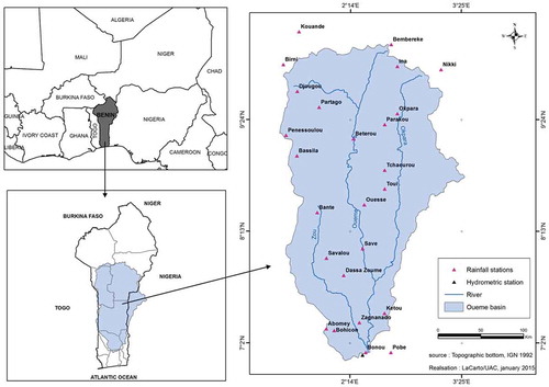
The Ouémé River basin at the Bonou outlet covers a surface area of 49 256 km² between 6.8–10.2°N latitude and 1.3–3.45°E longitude (Fig. 1). The Ouémé catchment covers two climatic zones: the Guinea savanna zone and the Soudanese savanna zone. The north of the catchment has a unimodal rainfall season (from mid-March to October) which peaks in August, whereas the south of the catchment exhibits a bimodal rainfall season (March–July and August–October) which peaks in June and September. This study is conducted, specifically, in the Bonou catchment of the Ouémé River. The inter-annual rainfall average on the Ouémé at Bonou is around 1100 mm, the minimum is 652 mm (in 1983) and the peak is 1536 mm (in 1963) over 1961–2010. On a global scale, Benin extends from the Niger River to the Atlantic Ocean, with relatively flat terrain, small mountains (about 600 m), and low coastal plains with marshlands, lakes and lagoons. The landscape is characterized by forest, gallery forest, savanna, woodlands, and agricultural as well as pasture land. Rainfall–runoff variability is high in the catchment, leading to runoff coefficients varying from 0.10 to 0.26, with the lowest values for the savanna and forest landscapes (Diekkrüger et al. 2010). Meteorological data (daily rainfall data and daily potential evapotranspiration, calculated by the Penman formula) and daily discharge data were provided, respectively, by the Benin Meteorological Department, ASCENA (Agency for Air Navigation Safety in Africa and Madagascar) and the National Directorate of Water (DG-Eau). A total of 25 rainfall stations are considered. In fact, a Kruskal-Wallis homogeneity test (Saporta 1974) was conducted on every station of the study area, which allowed these 25 stations to be retained. This test ensures that spatial homogeneity of the rainfall can be assumed. Moreover, the period 1961–2010 was chosen as the reference (a good compromise, taking into account the length of the data available for the different stations). Spatialized regional daily mean rainfall was obtained by kriging (Matheron 1970) with an exponential variogram of 53 km range, 0.3 nugget and 1 as the sill.

Figure 1. Study area and the hydrometeorological stations used.

3.2 Simulation of discharge with HyMoLAP

Model calibration was performed on the period 1990–1993 and the years 1994–1995 were used for model validation. In order to evaluate the model performance for the calibration and the validation, the following criteria were taken into account: the coefficient of model efficiency CE (Nash and Sutcliffe 1970), the coefficient of determination R² and the absolute percentage bias (APB). Figure 2 shows the result of the simulated hydrograph compared with the observed discharge for the calibration period, whereas Figure 3 presents the same data for the validation period. The difference between the observed and simulated results can be seen by a simple visual control and the numerical values for CE, R² and APB as presented in Table 1. The recession curve is quite well simulated. However, the uncertainties associated with the peaks are greater than those associated with low flow.

Table 1. Performance criteria of the hydrological model based on the least action principle (HyMoLAP) for the Bonou catchment, Ouémé River.

	CE	R^2	APB (%)
Model calibration (1990–1993)	0.85	0.89	33.5
Model validation (1994–1995)	0.87	0.86	38.6

Figure 2. Simulated hydrograph compared with the observed discharge (calibration) for the Bonou catchment.

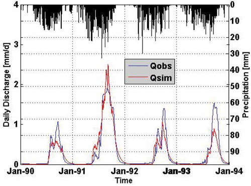
Figure 3. Simulated hydrograph compared with the observed discharge (validation) for the Bonou catchment.

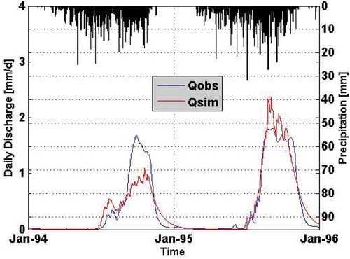
For both the calibration and the validation periods the CE and R² are greater than 0.85 (Table 1), while APB of 33.5% for the calibration period and 38.6% for the validation period were achieved. These results indicate that the HyMoLAP is suitable for simulation of river discharge in the Ouémé River basin. However, there are still many sources of uncertainty not being taken into account by HyMoLAP (for instance the uncertainties related to the random component of rainfall). This is the reason why the stochastic formulation of this model is preferred as the physical system behaviour is described in terms of probabilities. Thus, the lack of confidence (uncertainty) in the true discharge can be expressed using time-dependent probability distributions for the resulting discharge.

3.3 Tracking uncertainties

3.3.1 Assessment of the stochastic properties of the random component

As suggested by Equation (14), the stochastic properties of the random component must be investigated in order to have a more precise idea about the uncertainty associated with the model. This section therefore investigates the stochastic properties of the random component, ε_t, of rainfall. For ε_t to be white noise, the following conditions must be verified:

• E[ε_t] = 0,

• ε_t is Gaussian,

• ε_t has independent increments.

Investigation of the properties of the random component of rainfall is conducted through the implementation of some statistical tests. To this end, daily rainfall index, for the time period 1961–2010, is calculated as defined by Lamb (1982):

(15)

where q_t is the spatial averaged rainfall of day t, q̅ and σ_q represent, respectively, the mean and the standard deviation of this time series for the rainy seasons during the study period.

First, the validity of the assumption that the random component {ε_t} has zero mean is investigated. For this purpose a statistic, η(ε), is defined as:

(16)

where n is the number of observations, ε̅ is the estimate of the random component mean, and σ is the estimate of the random component standard deviation.

The statistic η(ε) is approximately distributed as t(α, n − 1), where α is the confidence level at which the test is being carried out (Mujumdar and Nagesh Kumar 1990). If the value of η(ε) ≤ t(α, n − 1), then the mean of the random component is not significantly different from zero. The values of the statistic η(ε) and t(α, n − 1) for the random component of rainfall for the Bonou catchment are, respectively, 0.0430 and 1.645. At the 95% confidence level, it is observed that the random component passes the test, leading to the conclusion that the random component mean value is not statistically different from zero (E[ε] ≈ 0).

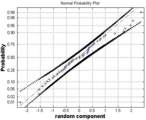
Second, the random component is checked for Gaussian properties using the normal probability plot (Chantarangsi et al. 2014). If the series follow a normal distribution, the data will fall within the confidence interval. The result of the Gaussian test for the distribution of the random component is shown by the normal probability plot (Fig. 4). All the data fall within the 95% confidence interval. Therefore, the data follow a normal distribution.

Figure 4. The normal probability plot with 95% confidence interval of the random component of rainfall for the Bonou catchment.

Third, the independence of the increments of the random component is investigated. The process ε_t is said to have independent increments if , , , …., are independent variables, where t₀ is the initial time and t₁, t₂, …, t_k are any times, with t₀ <  t₁ < … <  t_k (Liu 2008).

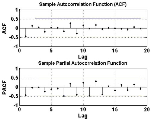
To this end, the autocorrelation function (ACF) and partial autocorrelation function (PACF) of the series of increments of the random component are computed for a maximum lag of 20 and a confidence level of 95% based on the sample size n. Two horizontal lines (blue lines) are superimposed at . These intervals give the acceptance region for testing the null hypothesis H₀: ρ_k = 0 at 5% significance level. They allow one to judge whether a particular ρ_k is statistically different from zero. The sample autocorrelation at lag k is defined as:

(17)

Figure 5 shows that the ACF and PACF for the series of increments of the random component of rainfall do not display any significant correlations. Therefore, the random component can be assumed to have independent increments.

Figure 5. Autocorrelation function (ACF) and partial autocorrelation function (PACF) for the series of increments of the random component of rainfall for the Bonou catchment. The horizontal lines give the threshold above which the correlation is significant at the level α = 0.05.

The above results show that the random component of rainfall over the Ouémé River basin can be approximated by white noise. We therefore conclude that this random component is also delta correlated and fulfils the condition that P(ε(0) = 0) = 1; it can also be represented as the time derivative (in the sense of a generalized function) of a stationary process with independent increments on non-overlapping intervals. White noise is commonly used in stochastic hydrology due to its simplicity and existing relationship to real processes.

3.3.2 Modelling the random component by white noise

The traditional approach for assessing the probability of outflow of a given frequency has been to pick a storm pattern, choose a runoff model and set the parameters with the best available estimate. One of the most important advantages of the SDE is the associated FPE, which allows one to directly derive the time-varying probabilities associated with the outflow.

Since ε_t can be treated as white noise, one can write Equation (8) in the form:

(18)

where .

In this case, the discharge Q is a Markov process and therefore the distribution function of discharge, P(Q,t), must obey Equation (19):

(19)

where ; stands for the correlation time of ε(t).

From Equation (19) a partial differential equation for P(Q,t) can be derived as the Kramers-Moyal expansion (Risken 1989):

(20)

where L_n are the moments of Q.

Formally, Equation (20) suggests that one may break off after a suitable number of terms. For instance, there could be situations where, for n > 2, L_n is identically zero or negligible (Risken 1989). In this case, one is left with the FPE:

(21)

where L₁ =  f(Q,t) and L₂ =  2G²(Q,t) stand, respectively, for the mean and the variance. Both L₁ and L₂ can be derived from Equations (12) and (14).

The FPE models the time evolution of the probability distribution in a system under uncertainty. In essence, the FPE is a conservation law expressing the fact that the probability distribution function (pdf) cannot be created or destroyed. Equation (21) corresponds to:

(22)

Equation (22) can be written in the form of a continuity equation:

(23)

where we have defined the probability current:

(24)

The evolution of the solution of the FPE is thus described by the hydrodynamic image of a continuous flow in discharge space. The corresponding current is the sum of the convection current, −fP, and the diffusion current, .

In a stationary state, P is independent of time t. As a consequence, J does not depend on Q. Thus, by integrating Equation (23) through applying, for instance, the variation of constants method, the normalized solution is obtained by setting J = 0.

(25)

where C is a constant.

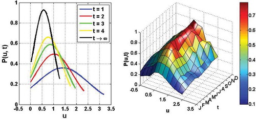
A remarkable feature is that a stationary state is a state that has no probability current. According to Annunziato and Borzì (2010), the state of a stochastic process can be completely characterized in many cases by the shape of its statistical distribution, which is represented by the pdf. For this reason, the time-dependent probability distributions for the resulting discharge are sought in the form of fundamental and approximate solutions of the associated FPE, Equation (21).

We define the fundamental solution as the solution that corresponds to the initial solution , in which the initial discharge Q₀ is well defined (not random). For simplicity, one can set μ = 1, γ = μ/λ such that f = γQ. The fundamental solution of the associate FPE, Equation (21), is given by Equation (26). Its derivation is given in Appendix A.

(26)

For t → ∞, the fundamental solution tends to the stationary distribution:

(27)

At each time t, during the wet seasons, the fundamental distribution is Gaussian with mean:

and variance:

These moments (mean and variance) can be derived from Equations (12) and (14). Using the standardized variables u of Q, that is:

(28)

for the time period 1961–2010, where σ_Q is the standard deviation of Q, the time-dependent probability distribution P(u,t) is plotted in Figure 6 for different times. At each time, the profile is symmetric about the expected value of the standardized discharge. It is also observed that the distribution becomes narrower with time.

Figure 6. Fundamental distribution P(u,t) of the standardized daily discharge u for the Bonou catchment for the period 1961–2010. The colours toward the blue end of the colour map indicate low probability and the colours at the red end of the colour map indicate high probability.

Now, the approximate solutions of the FPE (21) are sought. Indeed, the FPE does not have an explicit solution. It can be solved numerically or by approximation. Because extreme phenomena are analysed using the generalized extreme value (GEV) distribution, one seeks for an approximate solution that can be closed to the GEV law. Many studies have shown the use of the Hermite polynomial expansion to approximate the solution of the FPE (Alamou 2011). Hermite polynomials H_n(U) are orthogonal polynomials with respect to the standard Gaussian density defined over the interval (−∞, +∞).

The Hermite polynomials H_n(U) are defined by .

The Hermite polynomial expansion of the probability distribution is given in the form:

(29)

where A_i is the ith expansion coefficient expressed in terms of moments, r_i, of the variable u and given by , is the (i + 1)th Hermite polynomial, k represents the integer part of (i + 1)/2.

Thus,

Based on the above expressions of the expansion coefficients, the observed values of discharge are used to make calculations of P(u,t). Figure 7 shows the first four approximations.

Figure 7. Approximate distributions P(u,t) with Hermite polynomials up to order n = 4 of the standardized daily discharge u for the Bonou catchment, for the period 1961–2010. See Figure 6 for explanation.

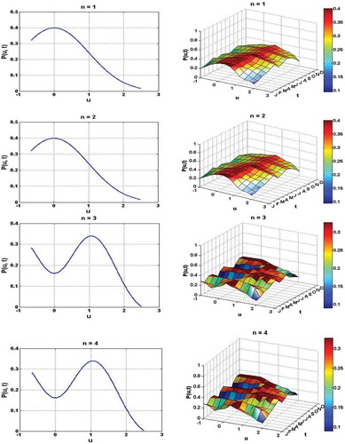
It can be seen that the first-order approximation, i.e. n = 1, leads to the case where E[U] = 0. As a result, the equation that describes the evolution of the variable u takes the form:

(30)

This result can also be predicted from Equation (22) when the term is equal to zero. In such a case, the distribution of the variable is Gaussian. The succeeding approximations (i.e. n = 2, 3 and 4) are corrected by their respective coefficients to give the corresponding shape of the solution of the FPE. Clearly, this result shows that for Gaussian PDF, only the diffusion current is considered, whereas for more complex PDF the convection current can be accounted for by successive terms of Hermite polynomials. The three-dimensional plot of the derived probability distribution is in accordance with the two-dimensional plot and, furthermore, the flow regime of the Ouémé River basin at Bonou is also reproduced.

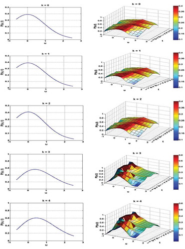
However, in this study, a new approximate solution can also be sought by using Student’s t distribution, which also belongs to the domain of attraction of GEV. The main motivation to choose Student’s t distribution is that it is also defined over the interval (−∞, +∞). Thus, one can write P(Q,t) as:

(31)

where ζ(Q) is the base density function, which is Student’s t distribution, given by:

(32)

in which β is the number of degrees of freedom of the distribution.

The term in Equation (31) denotes the associated orthogonal polynomials. The orthogonal polynomials associated with Student’s t distribution are given by (see Appendix B):

(33)

where is the moment of order k of the standardized variables u.

This equation shows that the leading Student’s t distribution term is corrected by higher-order contributions containing skewness and kurtosis excess. In the context of approximating the solution of the FPE, the coefficients a_k have to be determined so as to approach the solution of that partial derivative equation. Taking into account the properties of the derived polynomials, the coefficients a_k obey the optimal criteria defined in Galerkin’s method (Afouda et al. 2004). The time-dependent probability distributions for different order approximations are plotted in Figure 8. It can be noticed that the approximations for k = 0, 1 and 2 give the shape of Student’s t distribution. However, the approximations corresponding to k = 3 and 4 are corrected by the coefficients a_k and the shape of these solutions of FPE are reproduced accordingly.

Figure 8. Approximate distributions P(u,t) with orthogonal polynomials associated with Student’s t distribution up to order k = 4 of the standardized daily discharge u for the Bonou catchment, for the period 1961–2010.

We now want to investigate whether the different approaches used to derive the time-dependent probability distribution can be efficient in predicting the distribution of discharge. To this end, a comparison is made between the derived time-dependent probability distributions (fundamental and approximate distributions) and the empirical probability distribution of the standardized daily discharge. The standardized daily discharge u is arranged in descending order and ranks allotted. Then the estimated cumulative probabilities are computed using Hazen’s formula (Soro 2011):

(34)

where i stands for the rank of a value, and N is the total number of values to be plotted.

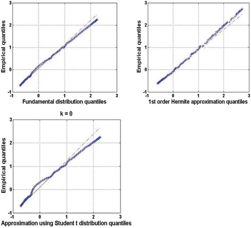
The empirical quantiles are plotted on the y-axis and the corresponding quantiles from the theoretically derived probability distributions are plotted on the x-axis. The quantiles of the derived probability distributions are computed based on the estimated associated cumulative probabilities. Figure 9 shows the quantile–quantile (Q–Q) plot for the standardized daily discharge. For the sake of brevity, only the results of the first order for the investigated approximations are presented. In this figure, it can be seen that the data points do tend to fall on the line.

Figure 9. Q–Q plot for standardized daily discharge for the Bonou catchment, for the period 1961–2010.

4 Discussion

As revealed by Equation (14), the evolution of the variance of the river discharge shows three terms:

• The first term,, describes the proper variance of the evolution of the discharge in the model output. This first term takes into account the model parameters and therefore quantifies both the uncertainties linked to the model structure and those linked to the model parameters.

• The second term, , quantifies uncertainties that are often not cited in hydrological literature but appear explicitly. These uncertainties are linked to the correlation between input ψ and output Q of the model.

• Finally the third term, , quantifies the uncertainties linked to the random component of rainfall.

To the best of our knowledge, the above result (Equation 14) is the first that explicitly shows the contribution of the input, model parameters and structural uncertainties in the output discharge. To emphasize the relevance of Equation (14), the proportion of the total variance that is attributable to each of the terms of Equation (14) has been calculated over the targeted catchment. The results revealed that the contribution of the first term to the total variance is 83.78%, while the second and third terms represent 10.62% and 5.60%, respectively. The proportion of the total variance that is attributable to both the second and third terms is the expected loss of precision when using the standard statistical theory over the investigated sub-catchment. The derived Equations (12) and (14) are designed to warn planners and decision makers that under climate change the mean and the variance are no longer constant parameters.

The performance of HyMoLAP has previously been compared with the GR4J model in the Ouémé at Bétérou catchment by Alamou (2011). This author found that HyMoLAP performs better than GR4J. However, the fact that the discharge peaks are not well simulated can be attributed to data errors (Andréassian et al. 2010, Kuczera et al. 2010). In fact, the improper representation of uncertainty is an intrinsic drawback of the deterministic hydrological models, since they do not include components that enable the preservation of the associated statistical characteristics of the observed data. Thus, using an appropriate random component of the inflowing rainfall can tackle the problem. As indicated in Efstratiadis et al. (2014), the nonlinearity of the resulting model induced by the deterministic model allows for a more faithful representation of the catchment behaviour and provides a better basis to exploit the available information, while the stochastic output is an advantage over the single output of the deterministic approach. This view is confirmed by the result given in Equation (14).

Under changing climate conditions, the river basin is a time-varying catchment and this is one of the reasons to understand the triple relationship between the input, the SDE that describes the river basin and the output. The approach using the FPE allows one to model the time evolution of the probability distribution in a system under uncertainty. At present, water resources planners in river basins are facing increased uncertainty in evaluating the hydrological conditions of the basins under climate change. The derived probability distributions of the model output show how the probability distribution changes over time and show more detail than do time series. The results of the time-dependent probability distributions presented in this study are mostly valid for the rainy season, as non-rainy days are omitted in the data series to fulfil the noise component assumptions.

In some systems, it may happen that these time-dependent probability distributions tend to a limiting stationary probability distribution when time evolves (Fig. 6). Therefore, in the steady state, the climate does not affect the probability distribution of the discharge. A comparison of the approximate solutions of the FPE revealed that the distribution of the standardized daily discharge with the first-order Hermite polynomials and the orthogonal polynomials associated with Student’s t distribution for the first three orders are close to Gaussian distributions. This shows the Gaussian character of the variable under study. The fact that the data points in the Q–Q plot for the standardized daily discharge tend to fall on the line indicates that the investigated time-dependent probability distributions are good models for the discharge data. By looking at the expression of the derived probability current, one can see that it is the sum of the convection current and the diffusion current. The modifications brought by the convection term to P(u, t) are contained in the successive terms of Hermite polynomials and orthogonal polynomials associated with Student’s t distribution. This convection term progressively changes the shape of the probability distribution of the standardized daily discharge, P(u, t).

5 Conclusion

The main contribution of this paper was to develop a rainfall–runoff modelling approach that aims to capture multiple sources and types of uncertainty in a single framework. The achievement of this analysis stemmed from the combination of a two-step modelling approach: (1) a deterministic modelling of the system dynamics by a hydrological model based on the least action principle (HyMoLAP); and (2) the stochastic formulation of HyMoLAP in terms of a stochastic differential equation (SDE). HyMoLAP is designed to minimize uncertainties related to the rainfall–runoff transformation process and scaling law, and thus is characterized by a limited number of parameters (λ, μ) capable of physical interpretation; while its stochastic formulation helps to make use of the large body of Ito stochastic differential equation theory and the associated FPE theory, now available for time-varying probability distribution derivation and uncertainty analysis.

Using data from Ouémé River basin (Benin), the properties of the random component of the inflowing precipitation have been investigated. This paper has shown that the white noise process and the associated Brownian motion can be an acceptable approximation to the random component of rainfall over the Ouémé River basin. The main advantage of the SDE approach is that it provides a physically transparent and mathematically tractable description of the stochastic dynamics, indicating how uncertainty in input precipitation and environmental parameters (potential evapotranspiration, temperature) affects the uncertainty in model output. Although the use of the SDE and the associated FPE as proposed in this paper can become more complex, the potential benefits in the areas of decision making, data collection and value of information are of promising importance.

Acknowledgements

The authors thank researchers and institutions who provided datasets for this work. The authors are also grateful to Dr Hountondji C. C. Fabien for his useful suggestions. We would also like to thank the three anonymous reviewers, as well as the Associate Editor, Dr Dieter Gerten, for their constructive comments and suggestions.

Disclosure statement

No potential conflict of interest was reported by the authors.

Additional information

Funding

The research leading to this work is funded by the West African Science Service Center on Climate Change and Adapted Land Use (WASCAL).

Appendix A  Derivation of the fundamental solution of the associate FPE

Let us define the Fourier transform with respect to Q for the fundamental solution:

(A1)

Since , then by applying the Fourier transform, the FPE becomes:

(A2)

One can show that the solution of Equation (25) is of the form:

(A3)

where is an arbitrary function chosen such that the initial solution is verified.

(A4)

Thus, Equation (A3) yields:

(A5)

Applying the inverse Fourier transform to Equation (A5), the fundamental solution of the FPE is:

(A6)

Appendix B  Derivation of the orthogonal polynomial associated with Student’s t distribution

To obtain the associated orthogonal polynomials, let us recall that Student’s distribution is part of the solution of Pearson differential equations. And it is well known that Pearson’s distribution leads to orthogonal polynomial systems when taking derivatives:

(A7)

where are real constants and = ; is a polynomial of degree 1.

All orthogonal polynomials can be obtained by repeatedly applying the differential operator as follows (Xiu and Karniadakis 2002):

(A8)

Equation (A8) is known as the generalized Rodriguez formula. These authors also showed that the weighting functions, ω(Q), for some orthogonal polynomials are identical to certain probability functions. That is why, in this approach, we choose Student’s t distribution as our weighting function. From Equation (A8), the well-known Hermite polynomials are obtained by taking R(Q) = 1. To derive expansion of the Student’s t distribution, which is part of the Pearson system, let us consider the polynomial of degree two, R(Q), as follows:

(A9)

Thus, using the above expression of R(Q) in the generalized Rodriguez formula, one derives the first five polynomials:

(A10)

It remains now to determine the constants a_k in Equation (31). This determination is just like that of the constants in a Fourier series and they are given by:

(A11)

Using the standardized variables:

where σ_Q is the standard deviation of Q, E[u] =0, E = 1 and E[u^k] = χ_k, one obtains the following coefficients:

(A12)

where χ_k is the moment of order k of the standardized variables u. Therefore, the orthogonal polynomials associated with Student’s t distribution are given by:

(A13)

References

- Afouda, A. and Alamou, E., 2010, Modèle hydrologique basé sur le principe de moindre action (MODHYPMA). Annales des Sciences Agronomiques du Bénin, 13 (1), 23–45.
- Afouda, A., Lawin, E., and Lebel, T., 2004. A stochastic streamflow model based on a minimum energy expenditure concept. In contemporary problems in mathematical physics: Proceeding 3rd Intern Workshop. Word Scientific Publishing, 153–169.
- Afouda, A., et al., 2007. Impact of climate change and variability on water resources in West African watersheds: what are the prospects? In: Synthesis Report - WRITESHOP, 21–24 February 2007.
- Alamou, E., 2011. Application du principe de moindre action a la modélisation pluie – débit. Thèse de Doctorat. CIPMA - chaire UNESCO, Université d’ Abomey Calavi.
- Andréassian, V., et al., 2010. Editorial – The Court of Miracles of Hydrology: can failure stories contribute to hydrological science? Hydrological Sciences Journal, 55 (6), 849–856. doi:10.1080/02626667.2010.506050
- Annunziato, M. and Borzì, A., 2010, Optimal control of probability density functions of stochastic Processes. Mathematical Modelling and Analysis, 15 (4), 393–407. doi:10.3846/1392-6292.2010.15.393-407
- Biao, I.E., et al., 2015, Influence of the uncertainties related to the random component of rainfall inflow in the Oueme river basin (Benin, West Africa). International Journal of Current Engineering and Technology, 5 (3), 1618–1629.
- Bodo, B.A., Thompson, M.E., and Unny, T.E., 1987. A review on stochastic differential equations for applications in hydrology. Stochastic Hydrology and Hydraulics, 1, 81–100. doi:10.1007/BF01543805
- Chantarangsi, W., et al., 2014. Normal probability plots with confidence. Biometrical Journal, 1–12. doi:10.1002/bimj.201300244.
- Cushman, J.H., 1987, Development of stochastic partial differential equations for subsurface hydrology. Stochastic Hydrology and Hydraulics, 1 (4), 241–262. doi:10.1007/BF01543097
- Denisov, S.I., Horsthemke, W., and Hänggi, P., 2009. Generalized Fokker – Planck equation: derivation and exact solutions. The European Physical Journal B, 68, 567–575. doi:10.1140/epjb/e2009-00126-3
- Diekkrüger, B., et al., 2010. Hydrology. In: P. Speth, M. Christoph, and B. Diekkrüger, eds. Impacts of global change on the hydrological cycle in West and Northwest Africa. Heidelberg, Germany: Springer, 60–64.
- Efstratiadis, A., Nalbantis, I., and Koutsoyiannis, D., 2014. Hydrological modelling of temporally varying catchments: Facets of change and the value of information. Hydrological Sciences Journal. doi:10.1080/02626667.2014.982123.
- Hanggi, P. and Ljung, P., 1995. Colored noise in dynamical systems. Advances in Chemical Physics, 89, 239–326.
- IPCC (Intergovernmental Panel on Climate Change), 2014a. Climate Change 2014: Impacts, Adaptation, and Vulnerability. Part A: Global and Sectoral Aspects. In: C.B. Field, et al. eds. Contribution of Working Group II to the Fifth Assessment Report of the Intergovernmental Panel on Climate Change. Cambridge, UK: Cambridge University Press.
- IPCC (Intergovernmental Panel on Climate Change), 2014b. Climate change 2014: impacts, adaptation, and vulnerability. Part B: regional aspects. In: V.R. Barros, et al. eds. Contribution of Working Group II to the Fifth Assessment Report of the Intergovernmental Panel on Climate Change. Cambridge, UK: Cambridge University Press.
- Khatri, K. B., 2013. Risk and Uncertainty analysis for sustainable urban water systems (PhD thesis). UNESCO-IHE, Delft, The Netherlands, 253 pages.
- Konecny, F. and Nachtnebel, H.P., 1995. A daily stream flow model based on a jump – diffusion process. In: Z. Kundzewicz, ed. New uncertainty concepts in hydrology and water resources. Cambridge: Cambridge University Press, 225–229.
- Koutsoyiannis, D., 2013. Hydrology and Change. Hydrological Sciences Journal, 58 (6), 1177–1197. doi:10.1080/02626667.2013.804626
- Kuczera, G., et al., 2010. There are no hydrological monsters, just models and observations with large uncertainties! Hydrological Sciences Journal, 55 (6), 980–991. doi:10.1080/02626667.2010.504677
- Kundzewicz, Z.W., et al., 2014. Flood risk and climate change: global and regional perspectives. Hydrological Sciences Journal, 59 (1), 1–28. doi:10.1080/02626667.2013.857411.
- Lamb, P.J., 1982. Persistence of Sub-Saharan drought. Nature, 299, 46–48. doi:10.1038/299046a0
- Liu, B., 2008, Fuzzy process, hybrid process and uncertain process. Journal of Uncertain Systems, 2 (1), 3–16.
- Matheron, G., 1970, La théorie des variables régionalisées et ses applications. Les Cahiers du Centre de Morphologie Mathématique de Fontaine Bleau Fascicule, 5, 212p.
- Mtundu, N.D. and Koch, R.W., 1987. A stochastic differential equation approach to soil moisture. Stochastic Hydrology and Hydraulics, 1, 101–116. doi:10.1007/BF01543806
- Mujumdar, P.P. and Nagesh Kumar, D., 1990, Stochastic models of streamflow: some case studies. Hydrological Sciences Journal, 35 (4), 395–410. doi:10.1080/02626669009492442
- Nash, J.E. and Sutcliffe, J.V., 1970. River flow forecasting through conceptual models part I – a discussion of principles. Journal of Hydrology, 10, 282–290. doi:10.1016/0022-1694(70)90255-6
- Risken, H., 1989. The Fokker – Planck Equation. Methods of solution and applications. 2nd ed. Berlin: Springer – Verlag, 472 p.
- Saporta, G., 1974. Probabilités, Analyse des données et statistique. Moscow: Mir.
- Serrano, S.E. and Unny, T.E., 1987. Semigroup solutions to stochastic unsteady groundwater flow subject to random parameters. Stochastic Hydrology and Hydraulics, 1, 281–296. doi:10.1007/BF01543100
- Soro, G.E., 2011. Modélisation statistique des pluies extrêmes en Cote d’ Ivoire. Thèse de Doctorat. Université d’ Abobo – Adjamé, 193 p.
- Strupczewski, W.G. and Mitosek, H.T., 1995. Some aspects of hydrological design under non – stationarity. In: Z. Kundzewicz, ed. New uncertainty concepts in hydrology and water resources. Cambridge: Cambridge University Press, 39–44.
- van Dam, J.C., 1999. Impacts of climate change and climatic variability on hydrological regimes. International Hydrology Series. Cambridge: Cambridge University Press.
- World Bank, 2011. Inondations au Benin: Rapport d’Evaluation des Besoins Post Catastrophe. Washington, DC: World Bank. Available from: http://documents.worldbank.org/curated/en/2011/04/1635839-inondations-au-benin-rapport-d’evaluation-des-besoins-post-catastrophes
- Xiu, D. and Karniadakis, G.E., 2002. The Wiener-Askey polynomial chaos for stochastic differential equations. SIAM Journal on Scientific Computing, 24 (2), 619–644. doi:10.1137/S1064827501387826