Simultaneous hydrological prediction at multiple gauging stations using the NARX network for Kemaman catchment, Terengganu, Malaysia

ABSTRACT

This paper presents a neural network model capable of catchment-wide simultaneous prediction of river stages at multiple gauging stations. Thirteen meteorological parameters are considered in the input, which includes rainfall, temperature, mean relative humidity and evaporation. The NARX model is trained with a representative set of hourly data, with optimal time delay for both the input and output. The network trained using 120-day data is able to produce simulations that are in excellent agreement with field observations. We show that for application with one-step-ahead predictions, the loss in network performance is marginal. Inclusion of additional tidal observations does not improve predictions, suggesting that the river stage stations under consideration are not sensitive to tidal backwater effects despite the claim commonly made.

EDITOR D. Koutsoyiannis ASSOCIATE EDITOR F. Pappenberger

KEYWORDS:

• Kemaman catchment
• multiple gauging stations
• NARX network
• one-step-ahead prediction

1 Introduction

Hydrological models are simplifications of physical hydrological processes based on our knowledge and understanding of a system. The mathematical representation of hydrological processes is highly complicated, involving many variables and system parameters (Singh and Woolhiser 2002). A physically-based model is thus typically complex and requires expensive computing time to solve the system partial differential equations (PDEs) (Yu 2002). In contrast, a conceptual model is a lumped model that uses spatially averaged parameters and thus does not take into considerations the heterogeneous characteristics of the hydrological system.

The artificial neural network (ANN) is a state-of-the-art tool that specializes in complex trend recognition from past examples. Unlike conventional time series predictions, such as autoregressive (AR) models, moving-average (MA) models, or the autoregressive moving-average model (ARMA), which are not designed to handle nonlinear signals (Diaconescu 2008), ANN models are universal approximators and are very much suited to dynamic and nonlinear modelling of hydrological systems (Abrahart and See 2007). Typical ANN models consist of three distinct layers, namely the input layer, the hidden layer(s), and an output layer, which are interconnected for complex mapping. The main advantage of this approach over the conceptual and physically-based hydrological models is that it does not require detailed understanding of the complex nature of the underlying processes to be explicitly described in mathematical form. ANNs can effectively deal with qualitative, incomplete and uncertain information, and are known to be fault tolerant and robust (ASCE 2000a, 2000b).

For over two decades, ANNs have been increasingly used in rainfall–runoff and streamflow modelling, collectively termed “river forecasting” (Abrahart et al. 2012). ANN models that are properly trained using historical data have been reported to function well in diverse applications related to hydrological systems. Amongst the popular network models are the feedforward back-propagation network (e.g. Campolo et al. 2003; Chiang et al. 2004, Wu et al. 2005), the multilayer perceptron (e.g. Senthil Kumar et al. 2005, Kalteh 2008, Mutlu et al. 2008), the radial basis function (e.g. Lin and Chen 2004, Senthil Kumar et al. 2005, Mutlu et al. 2008), fuzzy neural networks (e.g. Deka and Chandramouli 2005), the generalized regression model (e.g. Cigizoglu 2005, Lee and Tuan Resdi 2013), the recurrent neural network (e.g. Roy et al. 2010), and the NARX model (e.g. Arbain and Wibowo 2012, Ang et al. 2014).

Application of ANNs for rainfall–runoff modelling typically involves only a single point of interest where prediction is sought. For a large catchment with multiple points of interest, maintaining numerous standalone ANNs can be impractical and inefficient. Meanwhile, if simultaneous prediction is sought at these varied locations, the nonlinearity and complex dependencies of the problem inevitably increase due to the added temporal and spatial variability. Mutlu et al. (2008) introduced a method of hydrological predictions at multiple gauging stations which involved cascading the results obtained upstream in a catchment in the down-valley direction. Mehrvand and Nourani (2012) further showed that the approach by Mutlu et al. (2008) worked best with inputs of antecedent precipitation at the respective sub-basin instead of using uniform catchment-wide rainfall. However, performing runoff prediction at a downstream location based on predicted runoff at an upstream location may suffer from error propagation and error accumulation in the model. Another approach involves preprocessing input data into partitions that are adopted into separate models for each station (e.g. Wu et al. 2009, Demirel et al. 2012, Tsai et al. 2012, Nourani and Komasi 2013). More recently, Souza Júnior et al. (2015) introduced a two-tier regional model, which constitutes a middle way between the mainstream global model used to fit a single regression model and a localized model that fits multiple specialized regression models, each of which uses only a segment of the complete input data. Notwithstanding the above, a preferred alternative model is one that can process the catchment-wide input data from the hydrological network of stations and produce simultaneous prediction at multiple locations of interest.

The nonlinear autoregressive network with exogenous input (NARX) is a recurrent dynamic network, with feedback connections enclosing several layers of the network. As opposed to other recurrent ANNs, the feedback architectures in NARX are limited by the output neurons instead of the hidden neurons. This, however, does not incur any computational loss. As a matter of fact, the NARX model is more powerful and more practical (Horne and Giles 1995). It learns more effectively, converges and generalizes faster than other networks (Lin et al. 1996), and is far superior to linear models (Ali 2009). It has also been shown to excel in discovering long-term dependencies (Menezes and Barreto 2008) and capturing peak values (Chang et al. 2015), the latter of which is crucial in many applications, including flood prediction. The NARX network is essentially a class of dynamical models with computational power equivalent to Turing machines (Xie et al. 2009).

In this paper, our objective is to evaluate the ability of a NARX network on simultaneous prediction of hourly river stage at multiple gauging stations in a flood-prone catchment, which in this case is the Kemaman district in Terengganu, Malaysia. Specifically, we also examine the effect of the tidal breakwater, which is frequently cited by the authorities as the reason for major floods but lacks substantiation of data and scientific proof. The use of an hourly time scale allows us to incorporate the effect of fluctuating tidal water level on the observed river stage. Hourly prediction is also crucial for real-time flood forecasting during storm events, and has been reported by, amongst others, Wu et al. (2005), Tiwari and Chatterjee (2010), Tsai et al. (2012) and Demirel et al. (2012). The northeast monsoon in the tropics, which arrives in east-coast Peninsular Malaysia annually between November and February, for instance, frequently causes a fast-rising river stage posing a serious threat to the unsuspecting public and flood monitoring centres alike.

The paper is organized as follows. In Section 2 we provide the hydrological characteristics of Kemaman district and its present hydrological network. In Section 3 the architecture of the NARX network is described. Section 4 discusses the evaluation of the input parameters. Sections 5 and 6 present the network training and validation respectively. In Section 7 the network model is extended for one-step-ahead prediction, which in practical application translates to real-time advanced flood warning. In Section 8 the importance of tidal backwater effects for the river stages in the study area is examined. The performance of the NARX network model in simultaneous river stage prediction at multiple gauging stations using minimum training data length is concluded in Section 9.

2 Study area

The state of Terengganu, Malaysia, experiences flooding primarily due to monsoon rainfall. Kemaman district, in particular, consistently suffers annual flooding. For example, in December 2013 it was hit by the worst flood in 50 years which inundated nearly 80% of the district. River stage in the district was reported to exceed the danger level for an extended duration at a number of locations, namely Ban Ho Bridge, Air Putih Bridge and Tebak Bridge. It is often claimed that the flood was due to the combined effect of heavy rains and tidal backwater due to a high tide (The Malaysian Insider 2012, The Star 2013). Gasim et al. (2007) suggested that floods in Kemaman are aggravated by low water currents in the river regime, as well as a velocity and direction of wind that opposes the direction of river flow. However, no direct evidence was presented to support the claim.

The total area of Kemaman district in Terengganu, Malaysia, is 2535.59 km². It is located at latitudes 3°50ʹN–4°35ʹN and longitudes 102°50ʹE–103°40ʹE (Sulong et al. 2002). Its mean temperature ranges from a minimum of 21°C to a maximum of 31°C, and the average annual rainfall is estimated at 2500 mm/year. The hydrological network is widely established: there are ten rainfall stations, four river stage stations, one station measuring evaporation, and one station measuring mean relative humidity and temperatures. The geographical distribution of these stations is given in Figure 1 and their respective detailed locations and station IDs are listed in Table 1. The stations have been operational since as early as 1950, and as recently as 1986.

Table 1. Description of the network of hydrological of stations in Kemaman (Sources: DID, JUPEM and MMD).

Hydrological station	Station number	Unit	Month/Year operational	Location	Latitude/Longitude
Rainfall 1	4131001	mm	12/85	Ban Ho Village	04°08ʹ00ʺN/103°10ʹ30ʺE
Rainfall 2	4232104	mm	02/57	Pasir Gajah Primary School	04°14ʹ20ʺN/103°17ʹ50ʺE
Rainfall 3	4332001	mm	12/85	Tebak Bridge	04°22ʹ40ʺN/103°15ʹ45ʺE
Rainfall 4	4232002	mm	12/85	Air Putih Bridge	04°16ʹ15ʺN/103°11ʹ55ʺE
Rainfall 5	4333096	mm	03/57	Maternity Clinic at Ibok Village	04°19ʹ40ʺN/103°22ʹ05ʺE
Rainfall 6	3933001	mm	03/84	Hulu Jabor	03°55ʹ05ʺN/103°18ʹ30ʺE
Rainfall 7	4534092	mm	02/57	Kerteh Primary School	04°30ʹ30ʺN/103°26ʹ40ʺE
Rainfall 8	4434093	mm	02/57	Badrul Alam Shah Secondary School	04°25ʹ40ʺN/103°27ʹ05ʺE
Rainfall 9	4334094	mm	02/57	Kijal Primary School	04°19ʹ55ʺN/103°29ʹ15ʺE
Rainfall 10	4234109	mm	07/43	DID Kemaman	04°13ʹ55ʺN/103°25ʹ20ʺE
Evaporation	4333301	mm	11/83	Di Ketengah Town	04°21ʹ45ʺN/103°20ʹ50ʺE
Temperature	49465	°C	1950	Kemaman Hospital	04°14ʹ00ʺN/103°25ʹ00ʺE
Mean relative humidity	49465	mm	1950	Kemaman Hospital	04°14ʹ00ʺN/103°25ʹ00ʺE
Water level (Station 1)	4332401	m	05/86	Tebak River at Tebak Bridge	04°22ʹ40ʺN/103°15ʹ45ʺE
Water level (Station 2)	4232401	m	12/85	Kemaman River at Air Puteh Bridge	04°16ʹ15ʺN/103°11ʹ55ʺE
Water level (Station 3)	4232452	m	04/73	Kemaman River at Rantau Panjang	04°16ʹ50ʺN/103°15ʹ45ʺE
Water level (Station 4)	4131453	m	04/73	Cherul River at Ban Ho	04°08ʹ00ʺN/103°10ʹ30ʺE
Tidal water level	48507	cm	85	LKIM Complex, Chendering	05°15ʹ54ʺN/103°11ʹ12ʺE
Tidal water level	48485	cm	84	Port Kuantan, Tanjung Gelang	03°58ʹ30ʺN/103°25ʹ48ʺE

Figure 1. Distribution of hydrological network stations in Kemaman district.

The four river stage stations, referred to as Stations 1–4 herein, are located, respectively, on the Kemaman River at Rantau Panjang (station 4232452) and Air Puteh Bridge (station 4232401), on the Tebak River at Tebak Bridge (station 4332401), and on the Cherul River at Ban Ho (station 4131453). Station 3 is the confluence point of discharges from Stations 1 and 2 (see Fig. 1). Meanwhile, Station 4 is located in a separate sub-catchment. Flows from Stations 3 and 4 eventually converge and travel eastward into the South China Sea. Rainfall stations 1–4 are located in close proximity to the four river stage stations of interest, which are located inland. Rainfall stations 7–10, however, are distributed eastward along the coast. The evaporation gauging station is located away from the four river stage stations. Meanwhile, the station measuring temperature and humidity is located in Chukai town, near the coast, at the downstream end of the Kemaman River. The hydrological behaviour of the four river stage stations is summarized in Table 2.

Table 2. Hydrological behaviour of the river stage stations.

Station	Peak flow (m^3/s)	Base flow (m^3/s)	Base flow recession constant, Krb	Interflow recession constant, Kri
1	21.34	14.15	0.9998	0.8527
2	14.91	8.5	0.9997	0.8770
3	11.61	4.13	0.9998	0.9347
4	17.95	8.37	0.9996	0.9204

For the purpose of this study, the corresponding hydrological data were obtained from the relevant departments responsible for the respective stations, namely the Department of Irrigation and Drainage (DID) and the Malaysian Meteorological Department (MMD). We use hourly data chosen arbitrarily from 2009 to evaluate the present model. An initial training data length of 1 month is adopted to determine the ability of the model to produce accurate simulations with minimum training dataset.

3 The NARX network

One of the major difficulties in time series prediction using conventional ANNs is the failure to identify the underlying trend in the presence of outliers and seasonal variation. In addition, for a gradient-descent learning algorithm, it might be difficult to capture the immediate temporal effect with long-memory dependence (Diaconescu 2008).

In the NARX model, the next value of the dependent output signal is regressed on previous values of the output signal and previous values of an independent (exogenous) input signal, i.e. the model relates the required value of a time series to both the past values of the same series and the current and past values of an external driving series. The time delay thus effectively counters the problem of vanishing gradient by the propagation of past information.

In mathematical form, an NARX network model can be formulated as:

(1)

where x(n) ∈ R, and y(n) ∈ R represent the input and output of the model at discreet time step n, with d_x ≥ 1, d_y ≥ 1 (d_x ≤ d_y) being the orders of the memory vector of the input and output, respectively, and the parameter k (k ≥ 0) is a delay term known as the process dead-time (Xie et al. 2009). To solve for the nonlinear mapping function f, the model is popularly implemented as a feedforward time-delay neural network (Diaconescu 2008), or a standard multilayer perceptron (Xie et al. 2009, Shen and Chang 2013).

There are two modes for NARX network training. The parallel (P) mode feeds back estimated outputs to the input in a closed loop. The series-parallel (SP) mode, on the other hand, uses the actual values of the output system, thus giving the advantage of purely feedforward architecture, and allows static back-propagation in training. Figure 2 shows the typical architecture of the series-parallel mode used in this study. The open-loop configuration of the network is particularly useful for training purposes. The Levenberg-Marquardt (LM) algorithm has been identified to be the best learning algorithm for both training and validation in the NARX model and is adopted in the present study (Okkan 2011).

Figure 2. Typical serial–parallel (SP) architecture of NARX network, where Z^-1 is the unit time delay, is the estimated value.

4 Evaluation of input data

One major issue concerning ANN models is potential over-parameterization (Senthil Kumar et al. 2005). Another issue is the inherent black box treatment which renders the information contained in the trained network difficult to access and to interpret (Deka and Chandramouli 2005). A number of methods have been derived in order to assess the relative importance of the different inputs on the outputs, e.g. neural interpretation diagram (NID), Garson’s algorithm, and randomization approach (Kalteh 2008). An alternative simple approach is to evaluate the sensitivity of the output on the individual input dataset. For the Kemaman catchment, Tuan Resdi and Lee (2014) showed that, in addition to the rainfall data, accurate prediction of the river stages at Stations 1–4 in the catchment requires hydrological inputs such as temperature, humidity and evaporation. We now evaluate the relative importance of the available 13 hydrological inputs using hourly observations for 2009.

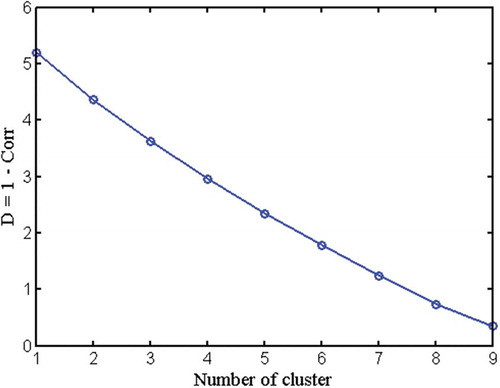
First, we adopt cluster analysis to identify the pattern similarity between the rainfall stations 1–10. The measure of dissimilarity D (= 1 – Corr) is computed based on the largest (complete linkage) difference of the correlation. Data linkage is then presented graphically using a dendrogram, i.e. a hierarchical tree showing the groups formed. Figure 3 shows the result of the groups and subgroups formed in the cluster analysis. It is observed that the 10 stations can be subdivided into two large groups: rainfall stations 1, 2, 10, 4 and 8 in one (Cluster A), and rainfall stations 3, 5, 6, 7 and 9 in another (Cluster B). The scree plot (Fig. 4), giving the dissimilarity vs the number of clusters, shows that there is no significant change in gradient (or “elbow” in the plot), suggesting that the 10 rainfall stations are near homogenous.

Figure 3. Dendrogram showing the dissimilarity and clustering of the 10 rainfall stations.

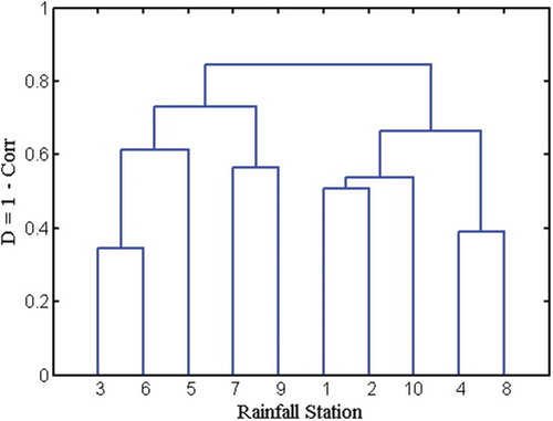
Figure 4. Scree plot showing total dissimilarity as a function of cluster number.

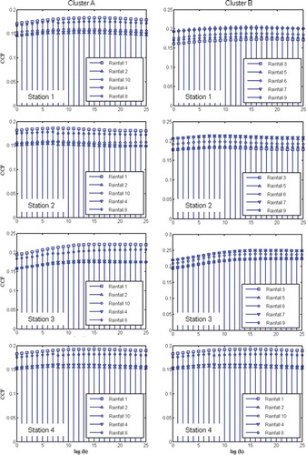
We proceed to examine the cross-correlation function (CCF) of each hydrological input on the water levels at gauging stations 1–4. Considering the results of the scree plot (Fig. 4), the rainfall stations in Clusters A and B are treated separately. Figure 5 shows the normalized cross-correlations of the rainfall stations in Clusters A and B to the water level stations 1–4. Overall, the highest CCF values between water levels and rainfall are typically observed for a lag of 6 hours (gauge station 2) to 15 h (gauge stations 1, 3 and 4), with values ranging between just under 0.2 to just above 0.25. The near uniform range of CCF values suggests that the difference between the effects of the two clusters on the river stage stations is insignificant. Hence, all the 10 rainfall stations should be considered as inputs for all the four water level stations, with a minimum of 6 h lead time.

Figure 5. Cross-correlation function (CCF) of rainfall stations in Cluster A (left column) and Cluster B (right column) on river stage stations 1–4 (top to bottom).

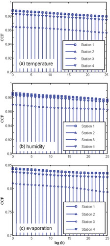
Figure 6 shows the CCF values between temperature (T), humidity (H) and evaporation (E) for the four gauging stations. High correlation is observed for all three inputs, with values well above 0.94 for T and H, and values of between 0.78 and 0.85 for E. Use of meteorological input, such as temperature (Demirel et al. 2012) and evapotranspiration (Ali 2009), for rainfall–runoff prediction has been shown to yield better results. Hence, we chose to include the complete set of 13 hydrological inputs in Table 1 in the present study.

Figure 6. Cross-correlation function (CCF) of (a) temperature, (b) humidity and (c) evaporation on river stage stations 1–4.

5 Network training

The network model is constructed and tested using MATLAB Neural Network Toolbox. For network training, we use 1-month hourly observations for the period 1–30 January 2009, which is subdivided for training (90%), validation (5%) and testing (5%). Network training is evaluated using the root mean square error (RMSE) and the coefficient of correlation (R):

(2)

(3)

where M is the total number of samples, Y_j and O_j are the values of predictions and observations, and and are their arithmetic means.

A standard NARX model has a single hidden layer of which the optimum number of neurons needs to be determined. Based on the findings in the preceding section, we first consider a NARX model where L_i = L_f = 6, L_i and L_f being the input delay and feedback delay numbers, respectively. Figure 7 shows that as the number of neurons increases, network performance improves at the expense of computation time. Specifically, for four neurons, the R value is observed to approach 1.000 for all four river stage stations, and the corresponding RMSE values are in satisfactory ranges, at 0.0168, 0.0144, 0.0286 and 0.0110, respectively for Stations 1–4.

Figure 7. Effect of number of neurons on (a) correlation coefficient (R) and (b) root mean square error (RMSE) (L_i = L_f = 6).

The importance of hydrological antecedent conditions cannot be overemphasized. Researchers have examined the effect of incorporating antecedent information of rainfall and river flow in order to produce accurate predictions (Senthil Kumar et al. 2005, Mutlu et al. 2008). Hence, we further examine the autocorrelation function (ACF) and partial autocorrelation (PACF) of the input data.

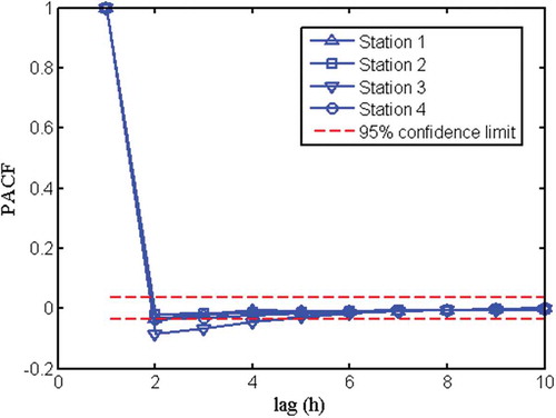
Figure 8 shows the ACF and PACF results for the rainfall stations. For Cluster A, the values of ACF fall below 0.1 for lag of 11 h or higher; for Cluster B, the values of ACF are observed to be very close for all the five stations except for 2 h lag and 3 h lag. Overall, the values of ACF are observed to be approximately equal to or less than 0.3 at lag 7 h or higher; hence, this is a suitable input delay for rainfall input. This is confirmed with the PACF, where the decaying pattern indicates reducing influence, especially beyond 10 h lag. The PACF values of the four water level stations are given in Figure 9. Other than that for Station 3, the PACF values generally fall close to or within the 95% confidence limit, and are entirely within this limit for lag of 6 h or higher.

Figure 8. Autocorrelation function (ACF) (top row) and partial autocorrelation function (PACF) (bottom row) of rainfall stations in Cluster A (left) and Cluster B (right).

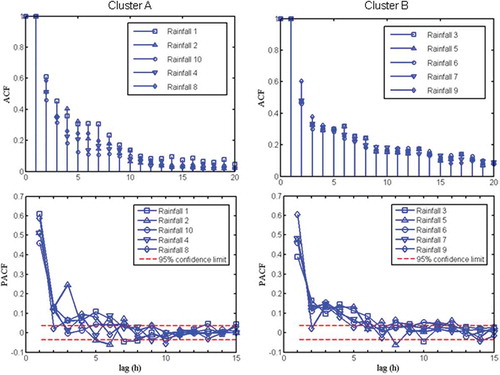
Figure 9. Partial autocorrelation function (PACF) of river stage stations 1–4.

Using the perturbation method, Sudheer (2005) showed that the tapped delay data Y_t−5 and Y_t−6 turned out to be insignificant in all ranges of flow, despite their high correlation with the required output. Keeping L_i = L_f, and four neurons in the hidden layer, we next consider the effect of different tapped delay on the model. Table 3 summarizes the R and RMSE values obtained for all four output stations. Results show that our present model performed best at L_i = L_f = 6. The finding agrees with Sudheer (2005), who showed that for hourly hydrological data, the most appropriate set of input vectors includes antecedent flows up to 6 h lag. Hence, the tapped delay of 6 h is adopted for all the 13 input parameters.

Table 3. Performance of the NARX model for different input delay and feedback delay (L_i = L_f; number of neurons in hidden layer = 4).

StationLi = Lf	1		2		3		4
	R	RMSE	R	RMSE	R	RMSE	R	RMSE
5	0.9963	0.0918	0.9949	0.0766	0.9957	0.1088	0.9984	0.0953
6	0.9999	0.0168	0.9999	0.0144	0.9999	0.0286	1.0000	0.0110
7	0.9999	0.3889	0.9999	0.4959	0.9999	0.6137	1.0000	0.6607

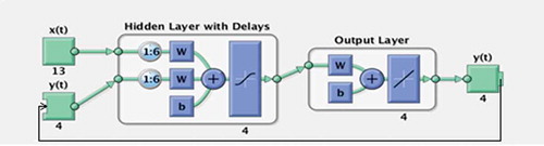
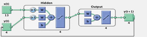
Figure 10 illustrates the resulting series–parallel (SP) NARX network model, which is a feedforward network with sigmoid transfer function in the hidden layer, and linear transfer function in the output layer. We note that the dependent output Y(t) is regressed on previous values of the output signal and the independent (exogenous) input signal.

Figure 10. Schematic diagram of the NARX network model.

6 Network validation

We validate the network developed in the preceding section on 1-month hourly observations for the subsequent months (February–December) in 2009. The simulated flow generally agrees well with the four river stage observations except specifically for the month of July (Fig. 11). It can be observed that only Station 3 produces reasonable prediction (R = 0.9894, RMSE = 0.0509). For Stations 1, 2 and 4, the recession curves are generally over-predicted.

Figure 11. Network validation for July 2009, showing poor predictions in recession curves.

Here, it is worth noting that one of the weaknesses of ANNs is extrapolation, i.e. performing simulation for a range of inputs that differ from the training datasets (Deka and Chandramouli 2005, Senthil Kumar et al. 2005). In particular, for a nonlinear and complex hydrological system, correct selection of training dataset is crucial to cover the broad spectrum of possible input scenarios. The poor results obtained for July 2009 suggest that the training dataset may not be sufficient to capture different catchment behaviour. Here, our strategy is to increase the training data length, which essentially allows the network to learn from more varied input conditions, such as high peaks, superposed peaks, flood recession etc. We note that while we attempt to develop the model with minimum historical data, there is no need to limit the length of the training dataset. An alternative but more tedious approach is to be more selective in identifying a minimal length of representative dataset.

Figure 12 plots the R and RMSE values for all four river stage stations with different input data lengths of 30, 60, 90 and 120 days, all of which begin with 1 January 2009 (e.g. 120 days input data for 1 January–30 April 2009). The results show that as network training data length increases from 1 to 4 months, there is no definitive trend in the R and RMSE values across all four water level output stations. This may be attributed to the fact that the output stations are physically scattered in the catchment, and thus their dependence on the input dataset varied due to spatial differences.

Figure 12. Effect of input data length on (a) correlation coefficient (R) and (b) root mean square error (RMSE) during network training.

Although the training test is inconclusive, we proceed to inspect the 1-month validation for July 2009. Figure 13 shows how the R and RMSE values vary with the input data length. The irregularity at lower data length indicates that the learning algorithm has yet to identify a general trend applicable to all the output stations. Table 4 shows performance of the NARX network trained using 120-day data. Significant improvement is observed for all four river stage stations. The river stage predictions for July 2009, as shown in Figure 14, are now significantly improved. The R values are well over 0.9934, and the RMSE values are below 0.0281.

Table 4. Validation results of the NARX model for July 2009 using different training data length (L_i = L_f = 6; number of neurons in hidden layer = 4).

Training data	Station	R	RMSE	SEE	R^2	NS
30 days (1–30 January 2009)	1	0.9918	0.1203	0.1761	0.8795	0.7029
	2	0.9799	0.1000	0.1012	0.8758	0.6977
	3	0.9894	0.0509	0.0366	0.9389	0.9773
	4	0.9872	0.0901	0.1298	0.8261	0.6393
120 days (1 January–30 April 2009)	1	0.9934	0.0281	0.0469	0.9929	0.9807
	2	0.9942	0.0123	0.0195	0.9980	0.9977
	3	0.9991	0.0142	0.0111	1.0000	0.9979
	4	0.9945	0.0135	0.0223	0.9930	0.9903

Figure 13. Effect of input data length on (a) correlation coefficient (R) and (b) root mean square error (RMSE) during network validation for July 2009.

Figure 14. NARX network validation for July 2009 using 120-day training dataset.

Further validation is conducted for the entire 8-month period of 1 May–31 December 2009, i.e. inclusive of the month of July 2009 for which erroneous predictions were reported earlier, where the total length of simulation is 245 days. Excellent predictions are produced for all four stations, with R > 0.9982 and RMSE < 0.0433 (Fig. 15).

Figure 15. NARX network validation for May–December 2009 using 120-day training dataset.

There is a possibility here that the chosen criteria, both R and RMSE, may not be providing an objective indication of model performance. Hence, network validation is further evaluated using additional measures, including the standard error of estimate (SEE), the coefficient of determination (R²), and the Nash-Sutcliffe (NS) criterion, defined as follows:

(4)

(5)

(6)

where is the mean flow over the period, and ν is the degree of freedom and is equal to the number of observations in the training set minus the number of parameters (Senthil Kumar et al. 2005). Note that the value of coefficient of determination R² is not the square of the coefficient of correlation R defined in Section 5.

Table 4 shows the validation results for July 2009 using 120-day comparisons to 30-day training data length. It is observed that the improvement in R value is minimal (of the order of less than 1.5%). For RMSE, SEE and R² values, the improvement is more readily noticeable, of the order of 10%. Meanwhile, NS values show the largest difference, where improvement of the order of 30% occurs for Stations 1, 2 and 4. The NS value for Station 3, which is already good, shows additional marginal improvement. These results show that, in the present model, the NS efficiency criterion is the most indicative of network performance, whereas the R value is the poorest.

In Table 5, the validation results for May–December 2009 using 120-day training data length are shown. Again we examine the improvement as shown by the above criteria. It is observed that both R (>0.9982) and R² (>0.9976) approach unity, whereas RMSE (<0.0433) and SEE (<0.065) approach zero. The NS criterion is well above 0.9960, suggesting that the network is well trained and efficient, with good overall performance.

Table 5. Validation results of the NARX model for May–December 2009 using 120-day training data length (L_i = L_f = 6; number of neurons in hidden layer = 4).

Station	R	RMSE	SEE	R^2	NS
1	0.9982	0.0299	0.0650	0.9998	0.9960
2	0.9992	0.0170	0.0316	0.9981	0.9984
3	0.9998	0.0433	0.0263	0.9989	0.9989
4	0.9992	0.0310	0.0446	0.9976	0.9983

At this point, we further compare the NARX model with a feedforward back-propagation (FFBP) network, a generalized regression network (GRNN), and a radial basis function network (RBFN). The optimum network architecture selected for each of the three networks is based on a previous report of Tuan Resdi and Lee (2014), and trained using the same 120-day dataset. The results show that the NARX network has the best performance, giving R > 0.9986, RMSE < 0.0048, SEE < 0.0672, R² > 0.9971 and NS > 0.9972 (Table 6). Although the RBFN model with spread constant 0.2 produces near comparable results, its SEE is generally higher than that of the present NARX model. The performance of the GRNN network with a spread constant of 0.1 is of even lesser quality, with noticeably higher SEE. Lastly, the FFBP network (I₁₃H_11,12,2O₄) is found to be totally unsuitable for the present application.

Table 6. Network training using 120-day data for FFBP, GRNN, RBFNN and NARX.

Neural network	Station	R	RMSE	SEE	R^2	NS
NARX (Delay = 6 h, number of neurons = 4)	1	0.9997	0.0552	0.0246	0.9990	0.9995
	2	0.9998	0.0193	0.0157	0.9991	0.9995
	3	0.9986	0.0250	0.0672	0.9971	0.9972
	4	0.9994	0.0430	0.0435	1.0000	0.9988
FFBP* (I13H11,12,2O4)	1	0.4741	1.0692	0.9556	0.1864	0.2216
	2	0.6077	0.5423	0.5910	0.2883	0.3634
	3	0.3818	0.9017	1.1836	0.0968	0.1370
	4	0.4631	1.2192	1.1212	0.1786	0.2117
GRNN* (spread constant = 0.1)	1	0.9785	0.2430	0.2269	0.8869	0.9561
	2	0.9874	0.1183	0.1184	0.9341	0.9744
	3	0.9822	0.2267	0.2431	0.9015	0.9636
	4	0.9793	0.2593	0.2595	0.8903	0.9577
RBFNN* (spread constant = 0.2)	1	0.9959	0.0969	0.0978	0.9918	0.9917
	2	0.9983	0.0436	0.0436	0.9965	0.9965
	3	0.9971	0.0977	0.0969	0.9942	0.9941
	4	0.9968	0.1004	0.1005	0.9936	0.9936

* Network design based on Tuan Resdi and Lee (2014).

7 One-step-ahead prediction

For hydrological application, such as river stage prediction, it is desirable to obtain the forecast at least one time step in advance. In the preceding model, Y(t + 1) is produced at the same time as it is given. For one-step-ahead prediction, Y(t + 1) is computed once Y(t) is available, but before the actual Y(t + 1) occurs. The network is made to return its output one time step early by removing one delay, i.e. the new network returns the same outputs as the original network, but outputs are shifted one time step. Figure 16 shows the schematic diagram of the one-step-ahead NARX model. Essentially, one-step-ahead predictors estimate the next value of a time series without feeding the predicted value back to the model’s input regressor. This means that the input regressor only contains actual sample points of the time series.

Figure 16. Schematic diagram of the NARX network model with one-step-ahead predictions.

Figure 17 shows the performance of the network model trained in the preceding section on one-step-ahead prediction for the 8-month period (245 days) of May–December 2009. Overall, the predictive results are only slightly poorer than the previous model (Fig. 15), with the coefficient of determination R² values being the least changed (Table 7). The R value and NS criterion reduce by up to 0.09% and 0.34%, respectively, whereas RMSE values deteriorate by up to 0.88%. The largest decline is observed in the SEE value, with a drop ranging from 3.4% to 4.8%. Overall, satisfactory one-step-ahead prediction allows the network to be deployed for actual flood warning purposes, providing crucial lead time for evacuation in the event of fast-rising river stage.

Table 7. Validation results of the one-step-ahead NARX model for May–December 2009 using 120-day training data length (L_i = L_f = 6; number of neurons in hidden layer = 4).

Station	R	RMSE	SEE	R^2	NS
1	0.9973	0.0360	0.1132	0.9985	0.9940
2	0.9975	0.0177	0.0799	0.9981	0.9950
3	0.9992	0.0521	0.0673	0.9989	0.9984
4	0.9987	0.0341	0.0789	0.9975	0.9974

Figure 17. NARX one-step-ahead predictions for May–December 2009.

8 Tidal backwater effects

Tidal backwater effects can have a dominant effect on storm discharge depending on astronomical and meteorological effects as well as the surface gradient of the flow pattern in the estuary of concern (DID 2000). Failure to consider the joint probability of combined coastal high water and extreme weather conditions can potentially lead to a disastrous outcome due to underestimation of the river stage. In the case of Kemaman, the chronic flooding has frequently been attributed, in part, to tidal high water, but the claim is lacking in substantive evidence.

The Department of Survey and National Mapping (JUPEM) operates and maintains two tidal stations along the coast of Terengganu, Malaysia, namely LKIM Complex, Chendering (Station 48507) (05°15ʹ54ʺN, 103°11ʹ12ʺE), and Port Kuantan, Tanjung Gelang (Station 48485) (03°58ʹ30ʺN, 103°25ʹ48ʺE). The two stations are located to the north and south, respectively, of the Kemaman River mouth (Fig. 18). Using the same 120-day (1 January–30 April 2009) trained model as before, we compare the preceding NARX network model with 13 hydrological input datasets (Model I) with the new model with two additional tidal input datasets (Model II). However, due to missing tidal observations at station LKIM Complex, Chendering (48507), we first performed hindcasting to replace the missing data for the period 15:00 h 11 December 2008 to 13:00 h 13 January 2009. Following the model by Lee (2007), we adopt a feedforward back-propagation network with network structure (I₁₀H₇O₁). Hourly simulations are produced for the period 1 December 2008 to 29 January 2009, with RMSE = 0.0026 and R = 0.9683, which are satisfactory (Fig. 19).

Figure 18. Tidal stations considered: Chendering (48507) and Kuantan (48485), nearest to the Kemaman River mouth.

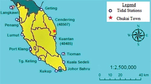
Figure 19. Hourly tidal hindcast using FFBP network (I₁₀H₇O₁) for tidal station 48507, showing replaced missing data for the period 15:00 11 December 2008 to 13:00 13 January 2009 (R = 0.9683, RMSE = 0.0026).

Table 8 summarizes the training results of comparing Model I and Model II using the same 120-day input data as before. It is observed that the two models both performed well, with Model I being marginally better. In order to further validate the network, prediction is performed for the same 245-day period (1 May 2009–31 December 2009). Here, Model I (R² > 0.9976, SEE < 0.0929 and NS > 0.9983) outperformed Model II (Table 9), suggesting that the tidal backwater effect is not important at the four river stage stations considered in the present study. The finding contradicts widespread claims in the past that the high tide was the main reason that the river system and drainage network overflowed.

Table 8. Comparison of NARX network training for Model I and Model II using 120-day dataset.

Station	Model I			Model II
	SEE	R^2	NS	SEE	R^2	NS
1	0.0672	0.9971	0.9972	0.0666	0.9972	0.9973
2	0.0157	0.9991	0.9995	0.0151	0.9995	0.9996
3	0.0246	0.9990	0.9994	0.0246	0.9989	0.9995
4	0.0435	1.0000	0.9988	0.0428	0.9986	0.9988

Table 9. Comparison of the NARX network validation for Model I and Model II for the period 1 May 2009–31 December 2009.

Station	Model I			Model II
	SEE	R^2	NS	SEE	R^2	NS
1	0.0650	0.9998	0.9960	0.0973	0.9921	0.9955
2	0.0316	0.9981	0.9984	0.0459	0.9922	0.9982
3	0.0263	0.9989	0.9989	0.0424	0.9931	0.9999
4	0.0446	0.9976	0.9983	0.0633	0.9901	0.9986

9 Conclusion

In this study, a NARX network is developed, trained and validated using 13 hydrological inputs datasets to produce four outputs of river stages in Kemaman catchment, Terengganu, Malaysia. The network model is designed based on network performance evaluated using root mean square error, coefficient of correlation, standard error of estimate, coefficient of determination, and the Nash-Sutcliffe efficiency criterion. The number of neurons in the hidden layer, and the input and output time delay were systematically chosen, and the minimum required input data length optimized. Network simulations for the year 2009 are in excellent agreement with field observations using a minimum 120-day training dataset. There is only a marginal decrease of network performance when applied for one-step-ahead network prediction, which translates to essential warning lead times during storm flood events. Overall, we conclude that the model can be used for simultaneous hydrological simulations at multiple gauging stations with satisfactory results, provided no significant change in land use of the catchment occurs. Meanwhile, the tidal backwater effect is found to be inconsequential in the performance of the model, suggesting its minimal influence on the river water level in Kemaman and, hence, debunking the widespread claims that flooding in this region is a coupled effect of rain and tidal high water.

Acknowledgements

The authors gratefully acknowledge the support given by the Research Management Institute (RMI), Universiti Teknologi MARA, Malaysia. We also would like to thank the anonymous reviewers for constructive feedback.

Disclosure statement

No potential conflict of interest was reported by the authors.

References

- Abrahart, R.J., et al., 2012. Two decades of anarchy? Emerging themes and outstanding challenges for neural network river forecasting. Progress in Physical Geography, 36 (4), 480–513. doi:10.1177/0309133312444943
- Abrahart, R.J. and See, L.M., 2007. Neural network modelling of non-linear hydrological relationships. Hydrology and Earth System Sciences, 11, 1563–1579. doi:10.5194/hess-11-1563-2007
- Ali, A., 2009. Nonlinear multivariate rainfall–stage model for large wetland systems. Journal of Hydrology, 374, 338–350. doi:10.1016/j.jhydrol.2009.06.033
- Ang, M.R.C.O., Gonzalez, R.M., and Castro, P.P.M., 2014. Multiple data fusion for rainfall estimation using a NARX- based recurrent neural network the development of the REIINN model. IOP Conference Series: Earth and Environmental Science, 17, 1–8.
- Arbain, S.H. and Wibowo, A., 2012. Neural networks based nonlinear time series regression for water level forecasting of Dungun River. Journal of Computer Science, 8 (9), 506–1513.
- ASCE, 2000a. Artificial neural networks in hydrology. I: preliminary concepts. Journal of Hydrologic Engineering, 5 (2), 115–123. doi:10.1061/(ASCE)1084-0699(2000)5:2(115)
- ASCE, 2000b. Artificial neural networks in hydrology. II: hydrologic applications. Journal of Hydrologic Engineering, 5 (2), 124–137. doi:10.1061/(ASCE)1084-0699(2000)5:2(124)
- Campolo, M., Soldati, A., and Andreussi, P., 2003. Artificial neural network approach to flood forecasting in the River Arno. Hydrological Sciences Journal, 48 (3), 381–398. doi:10.1623/hysj.48.3.381.45286
- Chang, F.-J., et al., 2015. Modeling water quality in an urban river using hydrological factors - data driven approaches. Journal of Environmental Management, 151, 87–96. doi:10.1016/j.jenvman.2014.12.014
- Chiang, Y.-M., Chang, L.-C., and Chang, F.-J., 2004. Comparison of static-feed-forward and dynamic-feedback neural networks for rainfall–runoff modeling. Journal of Hydrology, 290 (3–4), 297–311. doi:10.1016/j.jhydrol.2003.12.033
- Cigizoglu, H.K., 2005. Application of generalized regression neural networks to intermittent flow forecasting and estimation. Journal of Hydrologic Engineering, 10 (4), 336–341. doi:10.1061/(ASCE)1084-0699(2005)10:4(336)
- Deka, P. and Chandramouli, V., 2005. Fuzzy neural network model for hydrologic flow routing. Journal of Hydrologic Engineering, 10 (4), 302–314. doi:10.1061/(ASCE)1084-0699(2005)10:4(302)
- Demirel, M.C., Booij, M.J., and Kahya, E., 2012. Validation of an ANN flow prediction model using a multistation cluster analysis. Journal of Hydrologic Engineering, 17 (2), 262–271. doi:10.1061/(ASCE)HE.1943-5584.0000426
- Diaconescu, E., 2008. The use of NARX neural networks to predict chaotic time series. Wseas Transactions on Computer Research, 3 (3), 182–191.
- DID (Department of Irrigation and Drainage), 2000. Manual Saliran Mesra Alam. Kuala Lumpur: DID.
- Gasim, M.B.G., et al., 2007. Coastal flood phenomenon in Terengganu, Malaysia: special reference to Dungun. Research Journal of Environmental Sciences, 1 (3), 102–109. doi:10.3923/rjes.2007.102.109
- Horne, B.G. and Giles, C.L., 1995. An experimental comparison of recurrent neural network. In: G. Tesauro, D.S. Touretzky, and T.K. Leen (eds), Advances in neural information processing systems. 7th ed. Cambridge, MA: MIT Press, 697–704.
- Kalteh, A.M., 2008. Rainfall–runoff modeling using artificial neural networks (ANNs): modeling and understanding. Caspian Journal of Environmental Sciences, 6 (1), 53–58.
- Lee, W.K., 2007. Long term tidal forecasting and hindcasting using QuickTIDE tidal simulation package. J. Inst. Eng. Malaysia, 68 (2), 59–64.
- Lee, W.K. and Tuan Resdi, T.A., 2013. Neural network approach to coastal high and low water level prediction. Proceedings of the international civil and infrastructure engineering conference (InCIEC 2013), 22–24 September, Kuching, Malaysia, 275–279.
- Lin, G.-F. and Chen, L.-H., 2004. A Non-linear rainfall–runoff model using radial basis function network. Journal of Hydrology, 289, 1–8. doi:10.1016/j.jhydrol.2003.10.015
- Lin, T., et al., 1996. Learning long-term dependencies in NARX recurrent neural networks. IEEE Transactions on Neural Networks, 7 (6), 1424–1438.
- Mehrvand, M. and Nourani, V., 2012. An ANN-based data driven approach for multi-station rainfall–runoff modeling. International Journal of Computer Science and Management Research, 1 (4), 771–780.
- Menezes Jr., J.M.P. and Barreto, G.A., 2008. Long-term time series prediction with the NARX network: an empirical evaluation. Neurocomputing, 71 (16–18), 3335–3343. doi:10.1016/j.neucom.2008.01.030
- Mutlu, E., et al., 2008. Comparison of artificial neural network models for hydrologic predictions at multiple gauging stations in an agricultural watershed. Hydrological Processes, 22, 5097–5106. doi:10.1002/hyp.7136
- Nourani, V. and Komasi, M., 2013. A geomorphology-based ANFIS model for multi-station modeling of rainfall–runoff process. Journal of Hydrology, 490, 41–55. doi:10.1016/j.jhydrol.2013.03.024
- Okkan, U., 2011. Application of Levenberg-Marquardt optimization algorithm based multilayer neural networks for hydrological time series modeling. An International Journal of Optimization and Control: Theories & Applications (IJOCTA), 1 (1), 53–63.
- Roy, P., Choudhury, P.S., and Saharia, M., 2010. Dynamic artificial neural network modeling for flood forecasting in a river network. In: S. Paruya, S. Kar, and S. Roy (eds.). International conference on modeling, optimization, and computing (ICMOC), AIP Conference Proceedings, Vol. 1298(1), 219–225. doi:10.1063/1.3516305
- Senthil Kumar, A.R., et al., 2005. Rainfall-runoff modelling using artificial neural networks: comparison of network types. Hydrological Processes, 19, 1277–1291. doi:10.1002/(ISSN)1099-1085
- Shen, H.-Y. and Chang, L.-C., 2013. Online multistep-ahead inundation depth forecasts by recurrent NARX networks. Hydrology and Earth System Sciences, 17, 935–945. doi:10.5194/hess-17-935-2013
- Singh, V.P. and Woolhiser, D.A., 2002. Mathematical modeling of watershed hydrology. Journal of Hydrologic Engineering, 7 (4), 270–292. doi:10.1061/(ASCE)1084-0699(2002)7:4(270)
- Souza Júnior, A.H., Barreto, G.A., and Corona, F., 2015. Regional models: a new approach for nonlinear system identification via clustering of the self-organizing map. Neurocomputing, 147, 31–46. doi:10.1016/j.neucom.2013.11.046
- Sudheer, K.P., 2005. Knowledge extraction from trained neural network river flow models. Journal of Hydrologic Engineering, 10 (4), 264–269. doi:10.1061/(ASCE)1084-0699(2005)10:4(264)
- Sulong, I., et al., 2002. Mangrove mapping using landsat imagery and aerial photographs: Kemaman District, Terengganu, Malaysia. Environment, Development and Sustainability, 4 (2), 135–152. doi:10.1023/A:1020844620215
- The Malaysian Insider, 2012. Terengganu, Pahang facing second wave of flood. The Malaysian Insider, 31 Dec. Available from: http://www.themalaysianinsider.com/malaysia/article/terengganu-pahang-facing-second-wave-of-flood/
- The Star, 2013. Floods in Terengganu worsen, number of victims triple to over 22,000. The Star, 7 Dec. Available from: http://www.thestar.com.my/news/nation/2013/12/07/flood-tganu-worsen/
- Tiwari, M.K. and Chatterjee, C., 2010. Uncertainty assessment and ensemble flood forecasting using bootstrap based artificial neural networks (BANNs). Journal of Hydrology, 382, 20–33. doi:10.1016/j.jhydrol.2009.12.013
- Tsai, C.-C., Lu, M.-C., and Wei, C.-C., 2012. Decision tree-based classifier combined with neural-based predictor for water-stage forecasts in a river basin during typhoons: A case study in Taiwan. Environmental Engineering Science, 29 (2), 108–116. doi:10.1089/ees.2011.0210
- Tuan Resdi, T.A. and Lee, W.K., 2014. Neural network hydrological modeling for Kemaman Catchment. IEEE symposium on business, engineering & industrial applications (ISBEIA 2014), Sep 28–Oct 1, Kota Kinabalu.
- Wu, C.L., Chau, K.W., and Li, Y.S., 2009. Predicting monthly stream flow using data driven models coupled with data preprocessing techniques. Water Resources Research, 45, W08432.
- Wu, J.S., et al., 2005. Artificial neural networks for forecasting watershed runoff and stream flows. Journal of Hydrologic Engineering, 10, 216–222. doi:10.1061/(ASCE)1084-0699(2005)10:3(216)
- Xie, H., Tang, H., and Liao, Y.H., 2009. Time series prediction based on NARX neural networks: an advanced approach. In: Proceedings of the international conference on machine learning and cybernetics, 12–15 July. Baoding: IEEE Xplore Press, 1275–1279.
- Yu, Z., 2002. Hydrology: modeling and prediction. Encyclopedia of Atmospheric Sciences, 3 (980–986). doi:10.1006/rwas.2002.0172