Comparison of two rainfall–runoff models: effects of conceptualization on water budget components

ABSTRACT

Rainfall–runoff models with different conceptual structures for the hydrological processes can be calibrated to effectively reproduce the hydrographs of the total runoff, while resulting in water budget components that are essentially different. This finding poses an open question on the reliability of rainfall–runoff models in reproducing hydrological components other than those used for calibration. In an effort to address this question, we use data from the Glafkos catchment in western Greece to calibrate and compare the ENNS model, a research-oriented lumped model developed for the river Enns in Austria developed for the river Enns in Austria, with the operational MIKE SHE model. Model performance is assessed in the light of the conceptual/structural differences of the modelled hydrological processes, using indices calculated independently for each year, rather than for the whole calibration period, since the former are stricter. We show that even small differences in the representation of hydrological processes may impact considerably on the water budget components that are not measured (i.e. not used for model calibration). From all water budget components, direct runoff exhibits the highest sensitivity to structural differences and related model parameters.

EDITOR M.C. Acreman

ASSOCIATE EDITOR S. Huang

KEYWORDS:

• Rainfall–runoff model comparison
• water budget components
• parameter estimation
• Monte Carlo simulation

View correction statement:

Erratum

1 Introduction

Today, a large number of rainfall–runoff models are readily available to the hydrological community: e.g. Singh and Frevert (2006), and Beven (2012). Examples include the Sacramento Model (Burnash et al. 1973), TOPMODEL (Beven and Kirkby 1979), MIKE SHE (http://www.dhigroup.com/), HBV (Seibert and Vis 2012; mostly favoured in the Scandinavian region), and ARNO (Todini 1996) and TOPKAPI (Ciarapica and Todini 2002), commonly used in Italy. All these are conceptual models that simulate the runoff-contributing processes through a number of interconnected storages (see e.g. Chiew et al. 1993).

The main differences between conceptual models consist in the way the storages are interconnected, as well as the functional forms used to describe the hydrological processes in each particular model compartment. To that extent, several comparison studies have focused on quantifying how the quality of simulations is affected by data availability, hydro-climatic conditions, the characteristics of the catchment etc. For example, the WMO (1975) study applied 10 rainfall–runoff models to six different catchments, and compared them in terms of the physical concepts used, data and computer requirements, and level of accuracy under different hydro-climatic conditions; see Sittner (1976). In a similar setting, Chiew et al. (1993) compared two conceptual and four black box models by applying them to eight catchments, investigating the performance of runoff simulations over different time periods, the accuracy of low-flow estimates, and the efficiency of the representation of surface hydrology with respect to catchment characteristics. The effect of different modelling alternatives on simulation of low flows was investigated also by Staudinger et al. (2011), who compared four conceptual models and their variants. The effect of the spatial resolution of the data and the level of detail in modelling the hydrological processes on runoff simulations was investigated by Das et al. (2008), by comparing three versions of the same conceptual model (i.e. lumped-, semi-lumped and semi-distributed) using spatially varying meteorological data.

While the aforementioned studies shed light on the effects of different modelling assumptions on the simulated runoff hydrographs, an aspect not explicitly considered is the influence of different model structures on the specific components of the water budget: evapotranspiration, surface runoff, infiltration, interflow and groundwater discharge. Evidently, due to the modelling assumptions made in describing the hydrological processes, rainfall–runoff models calibrated to reproduce the measured river discharges (i.e. the total runoff) in a selected period may lead to different partitioning of the rainfall volume into the corresponding components of the water budget. This is due to the fact that model calibration based on measured river discharges cannot fully constrain the hydrological processes that contribute to the total runoff.

Since rainfall–runoff models are used not solely for simulation of the total runoff, but also for estimation of individual water budget components (i.e. evapotranspiration, surface runoff, infiltration, interflow and groundwater discharge), it is of practical importance to investigate under what conditions simulated water budget components that are not measured, or cannot be measured, are model dependent and should be treated with caution. This requires a comparative understanding of the effects of different modelling assumptions, as well as systematic and stringent testing of modelling alternatives (see e.g. Clark et al. 2011).

In an effort to bridge this gap, the present study (a) identifies the fundamental differences in the conceptual structures of two well-known and widely used models: ENNS (i.e. a relatively simple and easy to use research oriented lumped model; Nachtnebel et al. 1993) and the operational MIKE SHE (http://www.dhigroup.com/); (b) calibrates them for a selected period using data from the catchment of the Glafkos River in western Greece and quantitative measures to evaluate the simulation results; and (c) uses proper concepts to compare water budget components originating from the different conceptual structures of the two models, while assessing the importance and origin of the observed deviations.

In Section 2, we present some necessary details for the Glafkos catchment, the available data and their processing, and discuss how the model calibration period was selected. In Section 3, we outline the schematic representations used to model the hydrological processes in ENNS and MIKE-SHE, and present details of the underlying assumptions and relevant parameterizations. Section 4 investigates the effectiveness of a Monte Carlo procedure (see e.g. Duan et al. 1992, Wagener et al. 2004, Seibert and Vis 2012) combined with a multi-criteria evaluation approach (see e.g. Chiew et al. 1993, Ambroise et al. 1995, Madsen 2000, Madsen et al. 2002, Oudin et al. 2006, Clarke 2008, Das et al. 2008) for model calibration.

A thorough comparison of the results obtained is presented in Section 5, where we try to shed light to the observed differences in the simulated water budget components; i.e. evapotranspiration, infiltration through the unsaturated zone, and different components of the total runoff.

Finally, in Section 6 we test the efficiency of the two schemes in reproducing the measured discharges in the Glafkos catchment beyond the period of model calibration, and in Section 7 we discuss the main findings of this work.

2 The Glafkos catchment and available data

2.1 The catchment

The Glafkos catchment is located in western Greece and extends from the coast of the Gulf of Patras to the southeast slopes of the Panachaikon mountain; see Kaleris and Ziogas (2011) and Langousis and Kaleris (2013) for a detailed review. In this study, the focus is on the upper mountainous part of the catchment (see Fig. 1), with its outlet at the Glafkos diversion dam, located at an altitude of 340 m above mean sea level (a.m.s.l.). The storage capacity of the diversion dam is negligible. The area of this part of the catchment is 65.62 km², with mean elevation 1060 m and highest altitude of approximately 1800 m a.m.s.l. Concerning land use, sclerophyllous vegetation, transitional woodland-shrub, forest and agriculture cover more than 80% of the catchment area.

Figure 1. The Glafkos River catchment in western Greece.

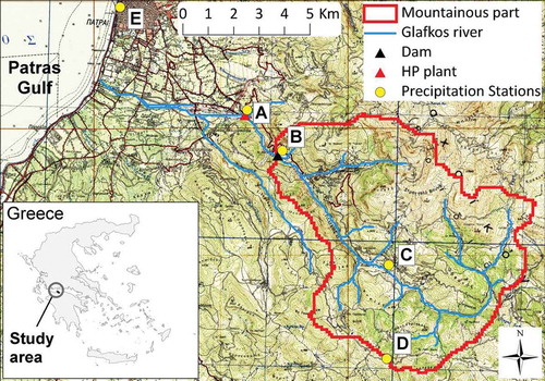
In the upper part of the catchment, small amounts of river water are abstracted directly from the riverbed for irrigation of small crop fields close to the river. The water at the outlet of the catchment is used (i.e. downstream from the diversion dam) for energy production, the water supply for the city of Patras, and irrigation. More precisely, from the diversion dam, a portion of the river flow is retained in the main stream for ecological purposes (i.e. environmental flow), and the remaining part is led through a pipeline to the hydro-electric plant of the Public Power Corporation (PPC), which is located approximately 2 km downstream from the dam (point A in Fig. 1), next to the river. Hence, daily river discharges at the catchment outlet are obtained as the sum of (a) the environmental flow retained in the main stream, (b) the water volume supplied to the hydro-electric plant and (c) in the case of very high discharges, the portion of water that flows over the spillway of the dam. The last portion of the river discharge is measured at the spillway.

During the wet period of the year (i.e. from November to April), a portion of the discharge at the outlet channel of the hydropower plant is directed, through a pipeline, to the water works of the city of Patras and used for fresh water supply. The rest of the water is returned to the riverbed, where a portion infiltrates and a portion discharges to the sea. During the dry period of the year, when the water demand of the city of Patras is fulfilled by groundwater, the largest portion of the discharge at the outlet channel of the hydro-electric plant is made available for irrigation of agricultural areas on the flat plain of Glafkos, and the remaining part, if any, is returned to the main stream. The aforementioned water uses highlight the significance of the Glafkos catchment hydrological budget, as it influences the availability of water resources in the Patras greater area, the third largest city in Greece.

2.2 Precipitation, temperature and runoff data

The study period includes hydrological years from 1974/75 to 1992/93, as this is the only period for which all the data required for the simulations are available: i.e. daily precipitation, temperature and river discharge. In Greece, each hydrological year starts on 1 October and ends on 30 September. Daily precipitation has been measured by the Public Power Corporation (PPC) at four sites; points A, B, C and D in Figure 1, located at altitudes of 181 340, 840 and 740 m a.m.s.l., respectively. To estimate the mean areal precipitation (MAP) needed for the rainfall–runoff simulations, we used the Thiessen-polygon method (see e.g. Dingman 2002, p. 121) and point rainfall measurements from stations B, C and D. The variation of the annual precipitation depth in the catchment for the study period is shown in Figure 2. During winter months, the upper part of the catchment receives precipitation in the form of snow.

Figure 2. (a) Spatially averaged annual precipitation (P) and measured annual runoff (RO) for the period from 1974/75 to 1992/93. (b) Comparison between the analytically estimated actual evapotranspiration (Turc’s method) and the difference (P − RO).

Daily mean temperatures are available from two stations of the Hellenic National Meteorological Service (HNMS) located in the city of Patras (point E in Fig. 1) at an elevation of 1 m a.m.s.l. and close to Araxos airport at an elevation of 15 m a.m.s.l. The latter is located about 30 km west of the city of Patras (not shown on the map).

Temperature time series exhibit two limitations: (a) daily measurements at Patras station are not complete, and (b) both stations record daily temperatures close to sea level, i.e. much lower than the mean elevation of the catchment (1060 m a.m.s.l.). To bypass these limitations we filled the missing values in the Patras temperature series using the corresponding measurements from Araxos station (see Ziogas 2006, Langousis and Kaleris 2013), and we used a pseudo-adiabatic lapse rate of 0.65°C/100 m to correct the resulting temperature series to account for the difference between the mean elevation of the catchment and the altitude at Patras station.

The discharge time series are complete (no missing values). However, the data have been corrected to eliminate sudden and intense drops in the measured runoff caused by abrupt operations at the energy production unit (see Langousis and Kaleris 2013). Note that the durations of abrupt operations are less than 1 day and, hence, they can be easily identified and eliminated, as the river discharge in the preceding and subsequent days is significantly higher. In addition, daily discharge measurements during the summer months, with values of about 0.25 m³/s, were found to exhibit irregular fluctuations. These fluctuations relate to the measuring accuracy (PPC, personal communication 2012), and were smoothed out by assigning a discharge value of 0.25 m³/s (note that the Glafkos River is a perennial stream with non-zero baseflow during all years in the record).

2.3 Selection of the calibration period

The period to be used for model calibration should be selected to minimize incompatibilities between the mean areal precipitation (MAP) used as model input and the measured runoff. Such incompatibilities occur when areal precipitation estimates are obtained from a small number of stations, as is the case here, where we use three stations. To check the compatibility between MAP and measured discharges, we apply the water budget equation at an annual level:

(1) $P-\mathrm{E}{\mathrm{T}}_{\mathrm{a}\mathrm{c}\mathrm{t}}=\mathrm{R}\mathrm{O}$(1)

where P, RO and ET_act are the annual precipitation and runoff depths, and actual evapotranspiration height, respectively. Equation (1) is based on the assumption that the annual change of storage in the catchment is negligible. Since catchments usually behave as linear reservoirs, the assumption above is supported by the small differences in the measured discharges at the beginning and end of all years in the record.

Figure 2(a) shows mean areal precipitation depth, P, and annual runoff height, RO, at the outlet of the catchment for the whole investigation period (i.e. from 1974/75 to 1992/93). The difference (P − RO), which according to Equation (1) should be equal to ET_act, exhibits significant fluctuations in time (see Fig. 2(b)). In order to assess these fluctuations, we compare them with those of the actual annual evapotranspiration calculated analytically using Turc’s empirical method (see Turc 1954, 1955, Shaw 1983, p. 259, Brutsaert 1984, p. 242). This method is commonly used in Greece for preliminary ET_act estimations (see e.g. Koutsoyiannis 1999, Karpouzos et al. 2011). Although Turc’s method (as all empirical methods) can provide only approximate (and possibly biased) estimates for the actual evapotranspiration, the magnitude of (P − RO) fluctuations (not exact values) relative to that of ET_act fluctuations, suffice to note that P and RO are not fully compatible for all the years on record (see also discussion in Section 6). Based on this observation, we consider that for time frames where the magnitude of (P − RO) fluctuations is similar to that of the fluctuations of the analytically calculated ET_act, the incompatibilities between P and RO are expected to be lower. Figure 2(b) shows such a period between 1984/85 and 1988/89, which we use for model calibration.

3 Rainfall–runoff models used

3.1 ENNS model

ENNS (Nachtnebel et al. 1993) is a research oriented lumped model, with conceptual structure shown in Figure 3. The input data are (a) precipitation, in the form of either rain or snow, and (b) temperature. The time scale of the inputs should match the time step of the numerical simulations, which in our case is daily. In the case when snow data are not available, precipitation is treated as snow when the air temperature drops below a lower threshold, usually taken to be zero. In ENNS, the snowmelt and refreeze modules follow a simple degree-day model, with coefficients that may differ and also vary in time. In this study, the melting and refreezing coefficients are taken to be equal to each other and constant in time.

Figure 3. Schematic representation of the conceptual structure of the ENNS model (Nachtnebel et al. 1993). Asterisks indicate modifications to the original interpretation of the corresponding hydrological processes.

The thickness of the soil zone (see Fig. 3) corresponds to the typical root depth of the vegetation in the catchment. The actual evapotranspiration, ET_act, is calculated by direct multiplication of the potential evapotranspiration, ET_pot, with three factors that take values between zero and one and account for the level of soil moisture, the precipitation depth and the snow cover. ET_pot is calculated using Thornthwaite’s analytical model (Shaw 1983, p. 263), where the mean temperature for each day on record is used to obtain a 30-day estimate of ET_pot, and the result is divided by 30.

Infiltration through the soil zone, which is responsible for groundwater recharge, is split into two components. The first component is the instantaneous percolation of rainwater and meltwater through the soil macropores, and it is proportional to (θ/θ_fc)^b, where θ is the actual water content, θ_fc is the water content at field capacity, and b is a constant estimated through model calibration. The other component is the time-dependent percolation through the soil matrix, which is modelled by approximating the soil zone as a linear reservoir with time constant k_inf. The latter is also estimated through model calibration.

Total runoff results from infiltration through the soil zone (Fig. 3), and it is modelled by three linear reservoirs, each one corresponding to a different component of the total runoff. According to Nachtnebel et al. (1993) and Eder (2002), the outflow from the horizontal outlet of reservoir 1 corresponds to the surface runoff (see Fig. 3). Note, however, that the outflow from reservoir 1 results from the water percolating through the soil zone, which contradicts the definition of surface runoff (see e.g. Chow 1964, p. 14-2). A more reasonable alternative is to consider the horizontal outflow from reservoir 1 as the direct runoff. The latter is defined as the sum of the surface runoff and the fast component of the interflow (see e.g. Chow 1964, p. 14-2). While not influential for ENNS, the modified interpretation of the hydrological processes modelled by reservoir 1 facilitates comparisons between the different runoff components produced by the two models (see also Section 3.2).

The vertical outflow from reservoir 1, which feeds reservoir 2, is controlled by time constant TVS1. According to Nachtnebel et al. (1993), the overflow from the horizontal outlet of reservoir 2 (see Fig. 3) corresponds to the interflow component of the total runoff. The latter is controlled by time constant TAB2 and, similarly to reservoir 1, occurs when the water depth in the reservoir exceeds the elevation threshold H2.

Table 1. ENNS model parameters and their corresponding ranges of variation. Parameters varied during model calibration are shown in bold.

Process	Variable	Value/range
Snowmelting and refreezing	CT (mm/d per °C): degree-day coefficient	2^a
Soil zone (the zone from which evapotranspiration takes place)	M (mm): thickness θfc (–): water content at field capacity θwp (–): water content at wilting point β (–): exponent for infiltration through macropores kSZ (h): time constant of linear reservoir of soil zone	500–2000^b 0.23–0.40^c 0.15^c 1–17 4000–10 000^d
Direct runoff and percolation (reservoir 1 in Fig. 3)	TAB1 (h): time constant for direct runoff TVS1 (h): time constant for percolation Η1 (mm): threshold depth for direct runoff	1–100 1–100 0.0
Slow interflow and deep percolation (reservoir 2 in Fig. 3)	TAB2 (h): time constant for interflow TVS2 (h): time constant for deep percolation Η2 (mm): threshold depth for interflow	100–2500 100–2500 0.0
Baseflow (reservoir 3 in Fig. 3)	TAB3 (h): time constant for baseflow	1500–12000
Runoff smoothing (reservoir 4 in Fig. 3)	TAB4 (h): Time constant for runoff smoothing	0.1

^aModerately forested areas in April (WMO 1983, p. 5.49)

^bThe thickness of the soil zone has been taken as equal to the root depth (see Crow 2005)

^cDingman (2002, p. 225)

^dNachtnebel et al. (1993)

Table 2. Parameter ranges and optimal parameter sets of ensembles 1 and 2, investigated using the ENNS model.

	Parameter ranges ofensemble 1	Optimal parameter set ofensemble 1 PSE1	Parameter ranges ofensemble 2	Optimal parameter set ofensemble 2 PSE2
(1)	(2)	(3)	(4)	(5)
M (mm)	500–2000	1811	1437–1996	1861
θfc (–)	0.23–0.40	0.38	0.28–0.40	0.30
β (–)	1–17	3.8	3.8–16.7	9.5
kSZ (h)	4000–10000	9756	6524–9925	9450
TAB1 (h)	1–100	59.3	18.3–98.9	59.4
TVS1 (h)	1–100	48.4	4.48–82.5	19.0
TAB2 (h)	100–2500	945	345–2312	776
TVS2 (h)	100–2500	1479	127–2471	1530
TAB3 (h)	1500–12000	4700	1550–11934	3605

Table 3. MIKE SHE model parameters and their corresponding ranges of variation. Parameters varied during model calibration are shown in bold.

Process	Variable	Value/range
Snowmelting and refreezing	Degree-day coefficient (mm/d per °C) Min snow storage (mm) Max wet snow fraction	2^a 0 0.5
ET (Vegetation)	Leaf area index (–) Coefficient of interception (mm) Root depth (mm)	5^b 0.05^c 500–2000^d
Overland flow	Initial water depth (m) Μanning number (m^1/3/s) Detention storage (mm) Slope (–) Slope length (m)	0^e 10^f 0–12 0.3^g 700^g
Unsaturated zone (parameters used in Green and Ampt method)	Water content at saturation (–) Water content at field capacity (–) Water content at wilting point (–) Saturated hydraulic conductivity (m/s) Soil suction (m)	0.43–0.47^h 0.23–0.40^h 0.14^h 1.5–2.5 × 10^–7^i 0.16–0.22^j
Simplified macropore flow	Max bypass fraction Water content for reduced bypass flow Min water content for bypass flow	0.3^k 0.35^l 0.14^m
Interflow and deep percolation (reservoir (a) in Fig. 4)	Time constant kha (d) Time constant kva (d)	0.04–4.0^n 0.04–4.0^n
Baseflow (reservoir (b) in Fig. 4)	Time constant khb (d)	4–100^n
Baseflow (reservoir (c) in Fig. 4)	Time constant khc (d)	60–500^n

^aModerately forested areas in spring during snowmelt (WMO 1983, p. 5.49)

^bValue for mixtures of broadleaf forest and shrub (Dingman 2002, p. 297)

^cSee MIKE SHE User Manual (2009, p. 295)

^dCrow (2005)

^eNo initial water depth at the soil surface at the beginning of the hydrological year (1 October)

^fMIKE SHE User Manual (2009, p. 115)

^gEstimated from the digital elevation model of the catchment (see Athanasiadou 2011)

^hDingman (2002, p. 225)

ⁱDingman (2002, p. 331)

^jDingman (2002, p. 235)

^kBeven and German (1982)

^lEqual to the mean value of the field capacity

^mEqual to the wilting point

ⁿRanges as those used for the corresponding reservoirs of the ENNS model (see Table 2). The threshold depths H_a, H_b and H_c in Figure 4 have been set to zero for the reasons discussed in Section 4.2 regarding ENNS.

Figure 4. Similar to Figure 3, but for the MIKE SHE model.

To ensure consistency with our previous modelling assumption (i.e. that the horizontal outflow from reservoir 1 corresponds to direct runoff), we consider the horizontal outflow from reservoir 2 as the slow component of the interflow (see modified interpretation in Fig. 3), rather than its total amount, as suggested by Nachtnebel et al. (1993) and Eder (2002).

Reservoir 3 has a single horizontal outlet and it models, according to Nachtnebel et al. (1993), the baseflow. Since baseflow is defined as the sum of the slow component of the interflow and the groundwater discharge (see e.g. Chow 1964, p. 14-2), we interpret the outflow from reservoir 3 as the groundwater discharge (see modified interpretation in Fig. 3). The outflow from reservoir 3 is controlled by time constant TAB3. Finally, the outflows from reservoirs 1, 2 and 3 are directed to the river reservoir 4, which models the runoff routing (see Figure 3). Reservoir 4 has a single outlet, and its outflow is controlled by time constant TAB4.

3.2 MIKE SHE model

To be comparable with ENNS, for the purposes of this study, we use the MIKE SHE model as a lumped model with structure similar to that of ENNS (see Fig. 4). More precisely, the hydrological processes modelled include (a) overland flow (i.e. the flow on the soil surface), (b) infiltration through the unsaturated zone, (c) evapotranspiration, (d) interflow and (e) groundwater discharge (see Fig. 4). The input data for MIKE SHE are the time series of daily precipitation, temperature and reference evapotranspiration, ET_ref (see e.g. MIKE SHE User Manual 2009, p. 78). As ET_ref we use in this study ET_pot, as calculated in ENNS simulations (see Section 3.1). Further, similarly to ENNS, precipitation is treated as snow when the temperature drops below a certain threshold, which is set to zero (MIKE SHE User Manual 2009, p. 78).

To simulate overland flow, we use the module Simplified Overland Flow Routing (MIKE SHE User Manual 2009, p. 264). Explicit consideration of overland flow in MIKE SHE is one of the most important differences between the two models (see also Section 3.1 above).

For the processes in the unsaturated zone (UZ), we use the two-layer water balance method (see MIKE SHE User Manual 2009, p. 304). In the case when the groundwater table is far below the soil surface, as in the Glafkos catchment, the UZ is modelled using an upper layer with depth equal to the sum of the root depth and the thickness of the capillary fringe, and a lower layer that extends from the bottom of the upper layer to the groundwater table.

The processes that take place in the upper layer are (a) infiltration, which, similarly to ENNS, is modelled using two components: i.e. the flow through the macropores and the flow through the soil matrix, and (b) evapotranspiration. Groundwater recharge is modelled by the outflow from the lower layer.

For the infiltration through the macropores we use the Simplified Macropore Flow module (see MIKE SHE User Manual 2009, p. 330), where flow through the soil macropores is proportional to the net precipitation, with a proportionality coefficient that depends on the soil water content. This modelling assumption is similar to the concept used in ENNS (see Section 3.1 above). Infiltration through the soil matrix is modelled using the Green and Ampt method (see MIKE SHE User Manual 2014, p. 342), which is another essential difference between MIKE SHE and ENNS (see Section 3.1).

At each time step, actual evapotranspiration, ET_act, is calculated as the total amount of water available, hierarchically, in (a) wet and dry snow (ET_snow), (b) the plant canopy (ET_canopy), (c) surface storage (i.e. ponded water; ET_ponded) and (d) the unsaturated zone (ET_UZ) (see MIKE SHE User Manual 2009, Section 14.2.5). The value of ET_act is upper-bounded by the reference evapotranspiration ET_ref (see above and Section 3.1). The calculation of ET_act is also an essential difference between MIKE SHE and ENNS.

The water infiltrating through the soil matrix of the upper layer of the unsaturated zone, can be either stored in the lower layer (see above), when its water content is lower than the field capacity, or added to the saturated zone as groundwater recharge. The water infiltrating through the macropores is routed directly to the saturated zone (see MIKE SHE User Manual 2009, p. 119).

For simulation of the subsurface runoff, MIKE SHE allows for the option to define a cascade of interflow reservoirs and more than one baseflow reservoirs (see MIKE SHE User Manual 2009, Section 16.2.2). In order to ensure consistency with model ENNS, we modelled interflow using a single reservoir (i.e. reservoir (a) in Fig. 4). For the baseflow, we started our modelling attempts using a single reservoir (reservoir (b) in Fig. 4), but the calibration process indicated limitations in approximating the measured hydrographs. To bypass those limitations and more accurately simulate runoff, we added a second reservoir for baseflow (reservoir (c) in Fig. 4). In this case, the water percolating from the interflow reservoir (i.e. reservoir (a) in Fig. 4) is distributed equally to the two baseflow reservoirs.

To allow comparisons between the different runoff components calculated by the two models, one needs to introduce an ENNS-compliant interpretation for the hydrological processes modelled by MIKE SHE. Since the overland flow in MIKE SHE is calculated using a simplified routing scheme, linear reservoirs (a), (b) and (c) in Figure 4 should be linked to subsurface runoff, i.e. the fast and slow components of the interflow and groundwater discharge.

One option is to consider that the horizontal outflows from reservoirs (a) and (b) approximate the fast and slow components of the interflow, respectively, and use the outflow from reservoir (c) for groundwater discharge (see the modified interpretation of the processes modelled by MIKE SHE in Fig. 4). In this case, the horizontal outflow from reservoir 1 in the ENNS model (i.e. the direct runoff; see Section 3.1 and above) should be compared to the sum of the overland flow and the horizontal outflow from reservoir (a) in MIKE SHE (i.e. the fast component of the interflow). In a similar manner, and since MIKE SHE does not independently calculate the outflows from reservoirs (b), i.e. slow component of the interflow, and (c), i.e. groundwater discharge, one should compare the sum of the outflows from reservoirs (b) and (c) in MIKE SHE with the sum of the horizontal outflows from reservoirs (2) and (3) in ENNS. All correspond to the baseflow; see e.g. Chow (1964, p. 14–2) and discussion above.

4 Model calibration

4.1 Calibration methods and criteria

The ENNS and MIKE SHE models have been calibrated using different methods. For ENNS we have used a Monte Carlo approach (see e.g. Seibert and Vis 2012), whereas MIKE SHE has been calibrated manually, by trial and error. The Monte Carlo approach allows for systematic investigation of a large number of independent parameter combinations, whereas in the “trial-and-error” approach parameter variation is much more limited, guided by the experience of the modeller. While the Monte Carlo approach can be considered more objective, it cannot be implemented in the case of MIKE-SHE because access to the code is restricted, and the required runs cannot be automated. In the case of ENNS, we modified the original code (Nachtnebel et al. 1993) to automate the calibration procedure and also conduct various calculations, including estimation of water budget components and calculation of performance measures. For the latter purpose (i.e. to assess the effectiveness of runoff simulations), we use four widely used criteria (see e.g. Chiew et al. 1993, Oudin et al. 2006, Moriasi et al. 2007):

(2) $\mathrm{C}\mathrm{r}\mathrm{W}\mathrm{B}=\hspace{0.17em}\frac{{\sum }_{i=1}^m\left(Q_{\mathrm{o}\mathrm{b}\mathrm{s},i}-\hspace{0.17em}{Q}_{\mathrm{s}\mathrm{i}\mathrm{m},i}\right)\hspace{0.17em}}{{\sum }_{i=1}^m{Q}_{\mathrm{o}\mathrm{b}\mathrm{s},i}\hspace{0.17em}}$(2)

(3a) $\mathrm{C}\mathrm{r}\mathrm{Q}=1-\hspace{0.17em}\frac{{\sum }_{i=1}^m{\left(Q_{\mathrm{o}\mathrm{b}\mathrm{s},i}-\hspace{0.17em}{Q}_{\mathrm{s}\mathrm{i}\mathrm{m},i}\right)}^2\hspace{0.17em}}{{\sum }_{i=1}^m{\left(Q_{\mathrm{o}\mathrm{b}\mathrm{s},i}-\hspace{0.17em}\overline{Q_{\mathrm{o}\mathrm{b}\mathrm{s}}}\right)}^2\hspace{0.17em}}$(3a)

(3b) $\mathrm{C}\mathrm{r}\sqrt{\mathrm{Q}}=1-\hspace{0.17em}\frac{{\sum }_{i=1}^m{\left(\sqrt{(Q_{\mathrm{o}\mathrm{b}\mathrm{s},i}}-\hspace{0.17em}\sqrt{Q_{\mathrm{s}\mathrm{i}\mathrm{m},i}}\right)}^2\hspace{0.17em}}{{\sum }_{i=1}^m{\left(\sqrt{(Q_{\mathrm{o}\mathrm{b}\mathrm{s},i}}-\hspace{0.17em}\stackrel{‾}{\sqrt{Q_{\mathrm{o}\mathrm{b}\mathrm{s}}}}\right)}^2\hspace{0.17em}}$(3b)

(3c) $\mathrm{C}\mathrm{r}\mathrm{l}\mathrm{o}\mathrm{g}\mathrm{Q}=1-\hspace{0.17em}\frac{{\sum }_{i=1}^m{\left(\mathrm{l}\mathrm{o}\mathrm{g}{Q}_{\mathrm{o}\mathrm{b}\mathrm{s},i}-\mathrm{l}\mathrm{o}\mathrm{g}{Q}_{\mathrm{s}\mathrm{i}\mathrm{m},i}\right)}^2\hspace{0.17em}}{{\sum }_{i=1}^m{\left(\mathrm{l}\mathrm{o}\mathrm{g}{Q}_{\mathrm{o}\mathrm{b}\mathrm{s},i}-\overline{\mathrm{l}\mathrm{o}\mathrm{g}{Q}_{\mathrm{o}\mathrm{b}\mathrm{s}}}\right)}^2\hspace{0.17em}}$(3c)

where Q_sim,i and Q_obs,i are the simulated and observed daily runoffs, m is the number of days in a hydrological year, and overbars indicate annual means.

CrWB provides an estimate of the cumulated error (i.e. overall bias) of model simulations at an annual level, which compensates for errors at different time steps and, therefore, it cannot be used to assess the effectiveness of model simulations at a daily time scale. For the latter purpose, the criteria in Equations (3a)–(3c) are better suited.

Equation (3a) expresses the Nash and Sutcliffe (1970) criterion. According to Oudin et al. (2006), this criterion is more sensitive to high discharges, whereas the criterion in Equation (3c) (i.e. based on logarithmically transformed quantities) focuses more on runoff lows. The criterion in Equation (3b) uses the square root transformed flows to provide a more general picture of the overall hydrograph fit (Oudin et al. 2006).

A notable difference relative to previous studies (e.g. Chiew et al. 1993, Ambroise et al. 1995, Madsen 2000, Madsen et al. 2002, Oudin et al. 2006, Clarke 2008, Das et al. 2008), is that the criteria in Equations (2) and (3) are calculated independently for each year, rather than for the whole calibration period. In this way, we ensure a more thorough evaluation of the best performing parameter sets (i.e. since the efficiency of model simulations in worse performing years is not averaged out; see also Kaleris and Langousis 2012), but add some complexities in model calibration, since we need to compare a larger number of criteria values. To tackle this issue, we first refine our search to those parameter sets that satisfy the constraint:

(4) $\underset{i=1,\hspace{0.17em}\dots ,\hspace{0.17em}n}{max}\left|\mathrm{C}\mathrm{r}\mathrm{W}{\mathrm{B}}_i\right|\hspace{0.17em}\le a_{\mathrm{m}\mathrm{i}\mathrm{n}}$(4)

where the subscript i denotes the hydrological year, n is the number of years in the calibration period and a_min is a threshold for the model bias, and then rank the remaining parameter sets using either the criterion in Equation (5) or that in Equation (6):

(5) ${\left(\mathrm{C}\mathrm{r}\sqrt{\mathrm{Q}}\right)}_{\mathrm{m}\mathrm{e}\mathrm{a}\mathrm{n}}=\left[{\sum }_{i=1}^n{\left(\mathrm{C}\mathrm{r}\sqrt{\mathrm{Q}}\right)}_i\right]/n$(5)

(6) ${\left(\mathrm{C}\mathrm{r}\mathrm{Q}\mathrm{l}\mathrm{o}\mathrm{g}\mathrm{Q}\right)}_{\mathrm{m}\mathrm{e}\mathrm{a}\mathrm{n}}=\left[{\sum }_{i=1}^n{\left(\mathrm{C}\mathrm{r}\mathrm{Q}\right)}_i+{\sum }_{i=1}^n{(\mathrm{C}\mathrm{r}\mathrm{l}\mathrm{o}\mathrm{g}\mathrm{Q})}_i\right]/2n$(6)

For more details on the selection of the aforementioned constraints and criteria, the interested reader is referred to the Appendix.

4.2 Calibration of the ENNS model

Table 1 summarizes the most influential parameters of the ENNS model and their ranges of variation, as obtained from the literature (see footnotes in Table 1) and specific applications of ENNS to other catchments (see Nachtnebel et al. 1993, Mehleri 2008, Koutsougera 2010). Five of the parameters: the degree-day coefficient C_T, the water content at wilting point θ_wp, the threshold depths H1, H2 of reservoirs 1 and 2, respectively, and the time constant TAB4 of the reservoir 4 (see Fig. 3), are not varied. The C_T-value used (i.e. C_T = 2 mm/d per °C in Table 1) corresponds to moderately forested areas during snowmelt in spring (WMO 1983, p. 5.49). The estimation uncertainty of C_T is small compared to uncertainties originating from the absence of snow data for the catchment and, for this reason, it is not varied. For clay loam soils, which prevail in the Glafkos catchment, the θ_wp-value does not vary significantly (Dingman 2002, p. 225). Furthermore, the small size and concentration time of the catchment do not justify smoothing of the runoff hydrographs by stream routing. Hence, we selected a TAB4-value very close to zero (i.e. TAB4 = 0.1 h, see Table 1). Finally, the small size of the catchment (see Section 2.1) as well as the large daily variability in the measured hydrographs, which links to that of daily precipitation (see discharge peaks in Fig. 6), support a fast hydrological response, and for this reason we have set the runoff threshold depths Η1 and Η2 (see Fig. 3) to zero.

Table 4. Optimal parameters for the MIKE SHE model.

Parameter	Value
Depth of soil zone (mm)	1000
Detention storage (mm)	10
Water content at saturation (–)	0.47
Water content at field capacity (–)	0.35
Saturated hydraulic conductivity (m/s)	2.0 × 10^−7
Soil suction (m)	0.22
Time constant kha of reservoir (a) in Figure 4 (d|h)	2.5|60
Time constant kva of reservoir (a) in Figure 4 (d|h)	0.4|9.6
Time constant khb of reservoir (b) in Figure 4 (d|h)	27|648
Time constant khc of reservoir (c) in Figure 4 (d|h)	250|6000

Figure 5. Criteria values for the ENNS simulations using parameter sets PSE1 and PSE2, and for the MIKE SHE simulations. (a) CrWB, (b) CrQ, (c) $\mathrm{C}\mathrm{r}\sqrt{\mathrm{Q}}$ and (d) CrlogQ.

Figure 6. (a)–(e) Comparison of measured and simulated hydrographs using the ENNS and MIKE SHE models for the period from 1984/85 to 1988/89. (f) Annual runoff (RO) and change of storage.

To estimate the remaining parameters in Table 1, namely M, θ_fc, β, k_SZ, TAB1, TVS1, TAB2, TVS2 and TAB3, whose range is given for comparison purposes (see below) in column 2 of Table 2, we used a Monte Carlo approach: we assumed uniformity of model parameters within their corresponding ranges of variation (on uniform random sampling see e.g. Duan et al. 1992), and used the Latin hypercube sampling method (see e.g. Helton 1993, Helton and Davis 2003) to generate an ensemble of 1000 random parameter sets, hereafter referred to as ensemble 1. For the needs of random sampling, we used the SimLab 2.2 software (http://simlab.jrc.ec.europa.eu/).

For each of the 1000 parameter sets of ensemble 1, we executed the ENNS model for the 5-year calibration period from 1984/85 to 1988/89 (see Section 2.3). To obtain the initial conditions for each simulation (i.e. initial reservoir storage and outflow) we repeated the hydrological simulation of year 1983/84 five times (i.e. warming up period). To avoid excluding too many parameter sets, we set the threshold for model bias in Equation (4) to a_min = 0.15 (see e.g. Moriasi et al. 2007). From the 1000 parameter sets in ensemble 1, 71 satisfied the a_min constraint. Ranking of the 71 parameter sets, using either the values of ${\left(\mathrm{C}\mathrm{r}\sqrt{\mathrm{Q}}\right)}_{\mathrm{m}\mathrm{e}\mathrm{a}\mathrm{n}}$ in Equation (5) or the values of ${\left(\mathrm{C}\mathrm{r}\mathrm{Q}\mathrm{l}\mathrm{o}\mathrm{g}\mathrm{Q}\right)}_{\mathrm{m}\mathrm{e}\mathrm{a}\mathrm{n}}$ in Equation (6), led to very similar results (i.e. 13 out of the 15 parameter sets with the highest ranks were the same). Thus, the two selection approaches are to a large degree equivalent. To better evaluate the efficiency of the best performing parameter set (i.e. that with rank 1; see column 3 in Table 2), hereafter referred to as PSE1, Figure 5 shows the values of CrWB, CrQ, $\mathrm{C}\mathrm{r}\sqrt{\mathrm{Q}}$ and CrlogQ for all years in the calibration period. While the values of CrQ, $\mathrm{C}\mathrm{r}\sqrt{\mathrm{Q}}$ and CrlogQ are large enough (except for those in year 1988/89; see below for a discussion) to substantiate an acceptable fit to the measured hydrographs, we used the 15 parameter sets of ensemble 1 with the highest ranks to define narrower ranges for model parameter selection (compare columns 2 and 4 in Table 2), and generate a new ensemble of 1000 parameter sets; hereafter referred to as ensemble 2. This is a way to adaptively guide the random search towards a more feasible parameter space (see e.g. Duan et al. 1992). The best performing parameter set from ensemble 2 (i.e. that with rank 1, hereafter referred to as PSE2; see Table 2) produced approximately the same or slightly better results relative to PSE1; see Figure 5. Hence, we selected PSE2 (see Table 2, column 5) as the optimal parameter set to perform ENNS simulations.

4.3 Calibration of the MIKE SHE model

Table 3 summarizes the parameters used in MIKE SHE simulations to model the different hydrological processes (see Section 3.2). The parameters varied for model calibration are shown in bold. Selection of parameter values not varied and the ranges of those varied are described in the footnotes of Table 3. The ranges of linear-reservoir time constants, root depth and field capacity are the same as those used to calibrate ENNS.

The “trial-and-error” calibration procedure (see Section 4.1) has been supported by a local sensitivity analysis (variation of one parameter at a time). More details are given in Siambi (2012). The initial conditions for MIKE SHE simulations were obtained using the same warm-up procedure as for ENNS (Section 4.2). The purpose of the manual parameter variation was to identify a parameter set for MIKE SHE that produces simulations that satisfy the constraint in Equation (4), and are characterized by values of criteria ${\left(\mathrm{C}\mathrm{r}\sqrt{\mathrm{Q}}\right)}_{\mathrm{m}\mathrm{e}\mathrm{a}\mathrm{n}}$ and ${\left(\mathrm{C}\mathrm{r}\mathrm{Q}\mathrm{l}\mathrm{o}\mathrm{g}\mathrm{Q}\right)}_{\mathrm{m}\mathrm{e}\mathrm{a}\mathrm{n}}$ that are close to, or better than those of ENNS with parameter set PSE2 (see Section 4.1 and Appendix). The resulting best performing parameter set is shown in Table 4.

4.4 Comparison of total runoff hydrographs simulated by ENNS and MIKE SHE

To facilitate comparison between MIKE SHE and ENNS results, the values of criteria in Equations (2) and (3) resulting from the MIKE SHE simulations using the parameter set in Table 4 have been included in Figure 5. One sees that in what concerns model biases, both models produce comparable results. However, the values of CrQ and CrlogQ (characterizing high and low flows, respectively, see Section 4.1) are slightly smaller for MIKE SHE than for ENNS. It is therefore expected that for MIKE SHE simulations the $\mathrm{C}\mathrm{r}\sqrt{\mathrm{Q}}$-values (characterizing the overall hydrograph fit, see Section 4.1) should generally be lower than those of ENNS (see Fig. 5(c)). Figure 6 presents a detailed comparison of the measured hydrographs with those simulated using MIKE SHE and ENNS. Despite the differences in the $\mathrm{C}\mathrm{r}\sqrt{\mathrm{Q}}$-values, visual inspection confirms that both models demonstrate similar skill in modelling the total runoff for all years in the calibration period. The largest deviations between the measured hydrographs and those simulated by both models concern the runoff peaks. This is also indicated by the fact that the values of criterion CrQ are smaller than those of $\mathrm{C}\mathrm{r}\sqrt{\mathrm{Q}}$ and CrlogQ (see Fig. 5). A probable reason for these deviations is that the estimated mean areal precipitation (see Section 2.2) is not fully compatible with the measured runoff. These incompatibilities seem to be larger for year 1988/89, which exhibits values for all criteria in Equation (3) smaller than those found for other years (Fig. 5). For the comparison of water budget components presented in the next section, it is important to note that the annual change of water storage in the two models is much smaller than the total annual runoff (i.e. less than 10%; see Fig. 6(f)). This is also supported by the small differences in the measured discharges at the beginning and end of all years on record (see Fig. 6(a–e)).

5 Comparison of the water budget components produced by ENNS and MIKE SHE

5.1 Evapotranspiration

Figure 7(a) compares the actual evapotranspiration, ET_act, calculated by ENNS and MIKE SHE for hydrological year 1984/85. One sees that the two series exhibit similar long-term patterns (i.e. periods with low and high ET_act values) since, in both models, ET_act is calculated as a portion of the potential evapotranspiration (see Sections 3.1 and 3.2). Similar results have been obtained for all years in the calibration period; not shown here for brevity. To facilitate detailed comparison of model results, Figure 7(b) focuses on the 4-month period from 1 January 1985 to 30 April 1985. One sees that the different methods used by the two models to calculate ET_act (see Sections 3.1 and 3.2) lead to deviations in the daily values. There are days where the ENNS ET_act-values reduce abruptly, whereas the corresponding MIKE SHE results behave differently. In addition to the differences in the mechanisms feeding evapotranspiration, this is mainly related to the fact that in ENNS the ET_act-values in rainy days are multiplied by a correction factor that varies between zero and one depending on the rainfall depth (see Section 3.1). In MIKE SHE, where calculation of ET_act is done on the basis of the total amount of water available in different compartments of the catchment (see Section 3.2), the variation of ET_act with respect to the rainfall amount is less intense.

Figure 7. Comparison of the actual evapotranspiration simulated by ENNS and MIKE SHE: (a) and (b) daily values for year 1984/85, (c) annual values.

Further, there are rainy days, particularly during dry periods (see, for instance, the values at the beginning or end of the hydrological year in Fig. 7(a)), where the ENNS ET_act-values reduce or remain unchanged, whereas the corresponding MIKE SHE results increase considerably. This is related to the fact that in MIKE SHE the rainwater becomes immediately available for evaporation, either as intercepted water or as ponded water on the soil surface (see Section 3.2), whereas in ENNS the increase of ET_act should be linked to an increase of the soil moisture and/or air temperature. This difference in the ET_act feeding mechanisms is the reason why the calibration of the two models results in significantly different thicknesses of the soil zone: i.e. 1860 mm for ENNS (see Table 2, column 5) and 1000 mm for MIKE SHE (see Table 4). In more detail, in ENNS only the water stored in the soil zone contributes to ET_act (see Section 3.1) and therefore the estimated soil thickness for ENNS is larger than that for MIKE SHE.

Despite the differences in the daily values, the annual ET_act depths calculated by the two models are very similar (see Fig. 7(c)), with the observed differences not exceeding 6%. This is a direct consequence of Equation (1) and two facts: (a) the two models are calibrated to produce similar hydrographs of the total runoff, and (b) the annual change of water storage in the catchment is small (much smaller than the total annual runoff, see Fig. 6(f) and Section 4.4). Note, however, that in cases when the annual change of storage is significant, measurements or reliable estimates of the annual ET_act become important for model calibration.

An additional note to be made here is that the simulated annual ET_act for the Glafkos catchment is from 25% to 40% smaller than that calculated using Turc’s analytical model (see Figure 7(c)). This is in accordance with the results presented in Figure 2(b), indicating that empirical estimates of ET_act should be considered with caution, as they might depend on the characteristics of the catchment, and the local hydro-climatic conditions.

5.2 Infiltration through the unsaturated zone

Figure 8(a) shows time series of infiltration obtained using the ENNS and MIKE SHE models for the typical year 1984/85. One sees that the infiltration time series exhibit similar long-term patterns, associated with days when precipitation and/or snowmelt occur. However, as in the case of ET_act (see Section 5.1), there exist deviations in the daily values.

Figure 8. Comparison of the total infiltration and its components simulated by ENNS and MIKE SHE: (a) total infiltration, (b) infiltration through the macropores, (c) infiltration through the soil matrix and (d) annual values.

More precisely, although the two models use the same method to calculate infiltration through the soil macropores (see Sections 3.1 and 3.2), the results obtained differ significantly: in ENNS almost all infiltration takes place through the soil macropores whereas in MIKE SHE macropore infiltration is less than half of the total (see Fig. 8(a) and (b)). These differences can be attributed to the different methods used by the two models in calculating the infiltration through the soil matrix (see Fig. 8(c)). Contrary to MIKE SHE, where partitioning of the infiltration is determined by a maximum bypass fraction of flow through the macropores and the parameters used in the Green and Ampt method (see Table 3), in ENNS there is no constraint on the bypass flow and infiltration through the soil matrix is calculated as the outflow from the linear reservoir of the soil zone (see Fig. 3 and Section 3.1). The latter is characterized by a time constant k_SZ, for which model calibration resulted in a very high value (see Table 2, column 4). Smaller values of k_SZ are not appropriate, since they allow for intense infiltration, also after the end of the wet period of the year, resulting in deviations between the measured and simulated hydrographs. High values of k_SZ cause the most of the infiltrating water to discharge through the soil macropores.

An additional observation is that almost no infiltration takes place at the beginning and end of the hydrological year (see Figure 8(a)). A similar finding has been obtained for all years in the calibration period (not shown here), and it implies that the unsaturated zone drains completely within a hydrological year (i.e. no change of storage in the unsaturated zone at an annual level).

Figure 8(d) compares the annual infiltration heights resulting from the two models. While partitioning of the total infiltration (i.e. to the soil matrix and macropores) is performed differently (see above), the observed differences in the annual infiltrated water volume do not exceed 6%. This can be explained by using the water balance equation in the unsaturated zone, which at the annual scale takes the form:

(7) $P-\mathrm{E}{\mathrm{T}}_{\mathrm{a}\mathrm{c}\mathrm{t}}-\mathrm{O}\mathrm{L}\mathrm{f}\mathrm{l}\mathrm{o}\mathrm{w}-\mathrm{I}\mathrm{n}\mathrm{f}=\mathrm{\Delta }{S}_{\mathrm{U}\mathrm{Z}}$(7)

where P, ET_act, OLflow, Inf, and ΔS_UZ denote the annual depths of precipitation, actual evapotranspiration, overland flow, infiltration, and storage change in the unsaturated zone, respectively. Since the change of storage in the unsaturated zone is negligible (see above), ET_act is approximately equal for the two models (see Section 5.1), and ENNS does not account for overland flow, it follows from Equation (7) that approximate equality of the annual infiltration volumes produced by the two models can occur solely in the absence of overland flow in MIKE SHE simulations. Since overland flow in MIKE SHE simulations may or may not occur depending on the hydrological conditions, the good correspondence of the two models in calculating the annual infiltration depth cannot be guaranteed a priori. This finding highlights the uncertain character of model-based results for infiltration and, further, demonstrates how the accuracy of the latter depend on the modelling assumptions made and the hydrological conditions used for model calibration.

5.3 Comparison of the runoff components

For the purposes of this study, the total runoff is considered to be the sum of direct runoff and baseflow (see Sections 3.1 and 3.2). In ENNS, direct runoff corresponds to the horizontal outflow from reservoir 1 (see Fig. 3 and Section 3.1), whereas in MIKE SHE (see Section 3.2) it corresponds to the sum of the overland flow and the horizontal outflow from the interflow reservoir (i.e. reservoir (a) in Fig. 4). In what concerns MIKE SHE simulations, no overland flow occurs in any of the years in the calibration period and hence the direct runoff in the Glafkos catchment calculated by MIKE SHE includes solely the horizontal outflow from reservoir (a) in Figure 4.

Figure 9(a) and (b) compares the direct runoff obtained from the ENNS and MIKE SHE models for the hydrological year 1984/85. Since direct runoff is directly influenced by total infiltration, the observed patterns are similar to those in Figure 8(a). In what follows, we refer to the annual depths of the horizontal and vertical outflows from reservoir 1 of ENNS and reservoir (a) of MIKE SHE (see Fig. 9(c)), in order to understand the observed differences in the daily values in Figure 9(a) and (b).

Figure 9. Comparison of (a, b) daily values and (c) annual values of the direct runoff simulated by ENNS and MIKE SHE.

As shown in Figure 9(c), the annual depth of direct runoff produced by ENNS (which corresponds to the horizontal outflow from reservoir 1) is significantly larger (more than 40%) than that of MIKE SHE, whereas the vertical outflow from reservoir 1 of ENNS is correspondingly smaller than that resulting from reservoir (a) of MIKE SHE. Evidently, the inflow to the aforementioned reservoirs of the two models (i.e. reservoirs 1 in ENNS and (a) in MIKE SHE), which corresponds to the infiltration from the unsaturated zone, is partitioned differently for horizontal and vertical outflows (see Fig. 9(c)). This difference in the partitioning is due to the different structures of reservoir 2 in ENNS and reservoir (b) in MIKE SHE: reservoir 2 is a two-outlet reservoir (Fig. 3), whereas reservoir (b) has a single horizontal outlet (Fig. 4). Due to this structural difference, the slow component of the interflow in MIKE SHE discharges directly to the river (Fig. 4), whereas in ENNS a portion of this component discharges directly to the river through the horizontal outflow from reservoir 2, and the remaining part discharges to the river through the groundwater reservoir (Fig. 3). This difference causes the contribution of the slow component of the interflow to the runoff peaks in MIKE SHE simulations to be stronger than that in ENNS. The reduced contribution of the slow interflow component to the peaks of total runoff in ENNS is compensated by larger values of direct runoff (i.e. horizontal outflow from reservoir 1). Evidently, the structural difference in reservoirs 2 (ENNS) and (b) (MIKE SHE) has a more general effect on the direct runoff and baseflow simulations, which is also reflected in the different values of the reservoir time constants obtained during model calibration (see column 5 in Table 2, and Table 4).

Similarly to direct runoff, the simulated daily values of the baseflow exhibit deviations (especially during the wet period of the year; see Fig. 10(a)), with the baseflow of MIKE SHE contributing more to runoff peaks than that of ENNS. This had been expected, since the baseflow in both models is calculated as the sum of groundwater discharge, and the slow component of the interflow (discussed above). However, the observed differences between the annual values of the baseflow (see Fig. 10(b)) are smaller than those of direct runoff; i.e. 4–12% for baseflow versus 34–46% for direct runoff (see above). Evidently, direct runoff is the water budget component that exhibits the highest sensitivity to the conceptual structures of the two rainfall–runoff models.

Figure 10. Comparison of daily and annual values of the baseflow simulated by ENNS and MIKE SHE.

6 Simulating runoff data beyond the calibration period

In this section we use the parameter sets in column 5 of Table 2 (for ENNS) and in Table 4 (for MIKE SHE) to obtain hydrographs of the total runoff for the period from 1975/76 to 1992/93, and compare them to those measured.

Figure 11 shows the values of criteria CrWB and $\mathrm{C}\mathrm{r}\sqrt{\mathrm{Q}}$ for the ENNS and MIKE SHE simulations. One sees that for most years the two models produce similar results. Significant deviations between measured and simulated hydrographs result for both models in years 1980/81, 1989/90, 1991/92 and 1992/93, as illustrated by the values of CrWB and $\mathrm{C}\mathrm{r}\sqrt{\mathrm{Q}}$. Concerning hydrological year 1980/81, the deficiency of both models in reproducing the measured hydrographs may be due to incompatibilities between precipitation and runoff data, or to inappropriate simulation of the snowmelt. Note that for hydrological year 1980/81, both models simulate an irregularly high annual depth of melt water (of the order 400 mm) relative to the remaining years (annual depth of melt water from zero to 170 mm). Thus, inappropriate simulation of the snowmelt can cause significant deviations in the simulated total runoff. This issue cannot be investigated in more detail due to lack of snow data in the Glafkos catchment.

Figure 11. Values of criteria CrWB, and $\mathrm{C}\mathrm{r}\sqrt{\mathrm{Q}}$ for the ENNS and MIKE SHE simulations for the years from 1975/76 to 1992/93.

For years 1988/89, 1989/90, 1991/92 and 1992/93, which are the driest in the period from 1975/76 to 1992/93 (see Fig. 2(a)), we tried to identify a parameter set that performs better. We repeated the automated calibration procedure for ENNS (see Section 4.2) for the period from 1988/89 to 1992/93. The procedure did not lead to parameter sets that produce better results. The most probable reason for the deficiency of both models in reproducing the measured hydrographs in these years is incompatibilities in precipitation and runoff data. A probable cause for these incompatibilities is unregulated water abstractions, upstream from the dam, for irrigation (see Section 2.1). The influence of such abstractions on measured discharges is maximized during dry periods (as in the period 1988/89 to 1992/93), when the river discharge is low.

Since the simulated hydrographs approximate the measured discharges equally well for 13 out of the 18 years in the simulation period, one may conclude that both models are appropriate for simulating the total runoff in the Glafkos catchment. However, as shown Figure 12, for the whole 18-year period, the two models produce different results for the direct runoff and baseflow: ENNS produces direct runoff values that are 30–46% larger than those of MIKE SHE, while the corresponding values of the baseflow are 3–13% smaller. This is in accordance with what was discussed in Section 5.3, highlighting the increased sensitivity of direct runoff to the conceptual structure and parameterization of the models.

Figure 12. Comparison of the annual depths of (a) direct runoff and (b) baseflow simulated by ENNS and MIKE SHE for the period from 1975/76 to 1992/93.

7 Summary and conclusions

A notable difference between rainfall–runoff models concerns the schematic structure and methods used to describe hydrological processes that contribute to the total runoff. As a result, hydrological models with different conceptual structures, calibrated to effectively reproduce the hydrographs of the measured runoff in a certain period, can be associated with water budget components (evapotranspiration, overland flow, infiltration through the unsaturated zone etc.) that deviate substantially. The origin and magnitude of the observed deviations are important issues that need to be understood and carefully addressed before evaluating and using the results obtained in hydrological impact studies.

In this work, we used the ENNS (a research oriented lumped model) and the operational MIKE SHE models to assess how different schematic representations of the hydrological processes affect model results. This was done for a catchment in western Greece, the Glafkos catchment (see Section 2.1).

Calibration of the ENNS model was based on a Monte Carlo approach and multiple evaluation criteria: i.e. the water balance error (model bias) and three variants of the Nash-Sutcliffe criterion, all calculated independently for each year of the calibration period. In order to avoid complexities in model parameter selection, we developed a simple to implement procedure for parameter selection that uses combined criteria based on cumulative sums (see Sections 4.1 and Appendix). For MIKE SHE, where access to the code is restricted, not allowing for automatic execution of a large number of simulations, model calibration was performed by trial and error (see Sections 4.1 and 4.3).

While the two calibrated models demonstrated similar levels of skill in reproducing the total runoff in the Glafkos catchment beyond the calibration period (see Section 6), the water budget components (i.e. evapotranspiration, infiltration and runoff) simulated by the two models differed significantly at the daily and/or annual time scales (see Section 5). To further understand the origins of the observed differences, we thoroughly investigated the schematic representations used in ENNS and MIKE SHE to model hydrological processes, concluding that:

1. The fundamentally different methods used by the two models to calculate the actual evapotranspiration result in different daily estimates, but in similar annual evapotranspiration depths. The latter is due to the fact that the annual change of storage in the catchment is small (see Fig. 6(f) and discussion in Section 2.3). Under these conditions the simulated annual evapotranspiration is approximately the same in both models, as it represents the portion of the rainwater removed from the runoff process. However, in cases when the annual change of storage is significant, reliable measurements (or estimates) of the annual evapotranspiration provide, in addition to the measured runoff, important information for the calibration of rainfall–runoff models.

2. The different methods used by the two models to simulate infiltration through the soil matrix of the unsaturated zone lead to significantly different partitioning of the infiltrated water volume (i.e. to the macropores and the soil matrix) and, consequently, to different daily estimates. The fact that in the present study the annual infiltration depths produced by the two models are approximately the same (see Section 5.2) cannot be considered indicative, as it is related to the specific hydrological conditions in the Glafkos catchment: no overland flow in the MIKE SHE simulations (see Section 5.2 and 5.3), and negligible annual change of storage in the unsaturated zone (see Section 5.2).

3. Although the total runoffs produced by the two models are similar and in good agreement with river discharge measurements, the daily and annual values of direct runoff and baseflow simulated by ENNS and MIKE SHE differ significantly. This finding originates from the structural differences of the linear reservoirs used in ENNS and MIKE SHE (see Sections 3.1 and 3.2 and Figs. 3 and 4), which affect the partitioning of infiltration from the unsaturated zone to baseflow and direct runoff, with the latter being more sensitive to model parameterization (see Section 5.3).

It is our opinion that the findings of this study pose an open question on the reliability of rainfall–runoff models in reproducing water budget components other than those used for calibration, and call for comparative understanding of the effects of different modelling assumptions on the calculated water budget components, The sensitivity of model parameter estimation to the temporal structure of rainfall, as embodied in the distribution of storm durations and intensities, will be the subject of a follow-up communication.

Acknowledgments

The authors would like to thank Professor H.-P. Nachtnebel for providing the original code of the ENNS model in Fortran, the Public Power Corporation (PPC) of Greece for providing discharge measurements from the Glafkos River, Dr D. Klotz, BOKU, Austria, for discussions on the linear reservoir equations of the ENNS model, K. Siambi for performing the MIKE SHE simulations, and A. Mamalakis and Dr A. Ziogas for preparing some of the figures. The authors would also like to thank the Associate Editor, Dr Shaochun Huang, for her in-depth review, detailed comments and suggestions that significantly improved the presentation of this work. The comments of Professor Semu Moges and an anonymous reviewer are also acknowledged.

Disclosure statement

No potential conflict of interest was reported by the authors.

Additional information

Funding

This research was financially supported by the Helmholtz Zentrum für Umweltforschung GmbH – UFZ, in Leipzig, Germany, under contract UFZ-02/2009 (RA-3205/9).

Appendix

Criteria used for model parameter selection

Selection of an optimal parameter set, based on the criteria values obtained when directly applying Equations (2) and (3) to each year in the calibration period is impractical, as (a) there is no unique parameter set that produces optimal values for a certain criterion for all years in the calibration period, and (b) for any given year, the optimal values for different criteria result from different parameter sets. It follows from (a) and (b) above that, even for a single year, there is no parameter set that simultaneously reproduces all aspects of the measured hydrographs in an optimal sense. In an effort to reduce the number of criteria in Equations (2) and (3) used for model parameter selection, we study their nonlinear dependence, and identify those that facilitate model parameter selection by incorporating additional information. More precisely, we use the ENNS simulations produced using the parameter sets in ensemble 1 to calculate the Spearman’s rank correlation coefficients (SRCCs, see e.g. Kottegoda and Rosso 1997) of CrQ, $\mathrm{C}\mathrm{r}\sqrt{\mathrm{Q}}$, CrlogQ and CrWB independently for each year in the calibration period (see Table A1).

One sees that all criteria are nonlinearly correlated at the 5% significance level (i.e. all values in Table A1 are larger than $1.96/\sqrt{N-1}=0.062$, for N = 1000), with CrWB (i.e. the model bias) exhibiting the weakest correlation with CrQ, $\mathrm{C}\mathrm{r}\sqrt{\mathrm{Q}}$ and CrlogQ. This was expected, since CrWB reflects the differences between observed and simulated annual runoff volumes, whereas CrQ, $\mathrm{C}\mathrm{r}\sqrt{\mathrm{Q}}$ and CrlogQ measure the deviations in the observed and simulated hydrographs at a daily level (see also Section 4.1). Thus, we use the constraint:

(A1) $\underset{i=1,\dots ,n}{max}\left|\mathrm{C}\mathrm{r}\mathrm{W}{\mathrm{B}}_i\right|\le a_{\mathrm{m}\mathrm{i}\mathrm{n}}$(A1)

where $\left|\mathrm{C}\mathrm{r}\mathrm{W}{\mathrm{B}}_i\right|$ is the absolute value of CrWB in hydrological year i, to identify parameter sets that do not exceed a lower threshold a_min in all years of model calibration (see below and Section 4.1).

Concerning the remaining criteria, $\mathrm{C}\mathrm{r}\sqrt{\mathrm{Q}}$ is strongly linked to both CrQ and CrlogQ (see Table A1). This implies that CrQ and CrlogQ include information at least partially embodied in $\mathrm{C}\mathrm{r}\sqrt{\mathrm{Q}}$. For this reason we use $\mathrm{C}\mathrm{r}\sqrt{\mathrm{Q}}$ as an additional criterion for model parameter selection. To smooth out variations of the $\mathrm{C}\mathrm{r}\sqrt{\mathrm{Q}}$-values in the different years, we use ${\left(\mathrm{C}\mathrm{r}\sqrt{\mathrm{Q}}\right)}_{\mathrm{m}\mathrm{e}\mathrm{a}\mathrm{n}}$, the mean value of $\mathrm{C}\mathrm{r}\sqrt{\mathrm{Q}}$ over the years used for model calibration:

(A2) ${\left(\mathrm{C}\mathrm{r}\sqrt{\mathrm{Q}}\right)}_{\mathrm{m}\mathrm{e}\mathrm{a}\mathrm{n}}=\left[{\sum }_{i=1}^n{\left(\mathrm{C}\mathrm{r}\sqrt{\mathrm{Q}}\right)}_i\right]/n$(A2)

where n is the number of years in the calibration period. Larger values of ${\left(\mathrm{C}\mathrm{r}\sqrt{\mathrm{Q}}\right)}_{\mathrm{m}\mathrm{e}\mathrm{a}\mathrm{n}}$ indicate parameter sets that better fit the measured hydrographs in the whole calibration period. Hence, one can combine the constraint $\underset{i=1,\dots ,n}{max}\left|\mathrm{C}\mathrm{r}\mathrm{W}{\mathrm{B}}_i\right|\le a_{\mathrm{m}\mathrm{i}\mathrm{n}}$ with the ranking of the ${\left(\mathrm{C}\mathrm{r}\sqrt{\mathrm{Q}}\right)}_{\mathrm{m}\mathrm{e}\mathrm{a}\mathrm{n}}$ values to identify parameter sets that perform well (see Section 4.2).

Since $\mathrm{C}\mathrm{r}\sqrt{\mathrm{Q}}$ does not embody all the information included in criteria CrQ and CrlogQ (see discussion above and Table A1), we have also tried replacing ${\left(\mathrm{C}\mathrm{r}\sqrt{\mathrm{Q}}\right)}_{\mathrm{m}\mathrm{e}\mathrm{a}\mathrm{n}}$for model parameter selection with a weighted criterion that focuses equally on runoff highs and lows:

(A3) ${\left(\mathrm{C}\mathrm{r}\mathrm{Q}\mathrm{l}\mathrm{o}\mathrm{g}\mathrm{Q}\right)}_{\mathrm{m}\mathrm{e}\mathrm{a}\mathrm{n}}=\left[{\sum }_{i=1}^n{\left(\mathrm{C}\mathrm{r}\mathrm{Q}\right)}_i+\hspace{0.17em}{\sum }_{i=1}^n{(\mathrm{C}\mathrm{r}\mathrm{l}\mathrm{o}\mathrm{g}\mathrm{Q})}_i\right]/2n$(A3)

Combined criteria based on cumulative sums have also been suggested by Madsen et al. (2002) and Oudin et al. (2006). In Section 4.2 we discussed our findings when using $\left|\mathrm{C}\mathrm{r}\mathrm{W}{\mathrm{B}}_i\right|$ and either ${\left(\mathrm{C}\mathrm{r}\sqrt{\mathrm{Q}}\right)}_{\mathrm{m}\mathrm{e}\mathrm{a}\mathrm{n}}$ or ${\left(\mathrm{C}\mathrm{r}\mathrm{Q}\mathrm{l}\mathrm{o}\mathrm{g}\mathrm{Q}\right)}_{\mathrm{m}\mathrm{e}\mathrm{a}\mathrm{n}}$ for model parameter selection.

Table A1. Spearman’s rank correlation coefficients (SRCCs) of criteria CrQ, $\mathrm{C}\mathrm{r}\sqrt{\mathrm{Q}}$, CrlogQ and CrWB, calculated independently for each year in the calibration period.

Year	SRCCCrQ, $\mathrm{C}\mathrm{r}\sqrt{\mathrm{Q}}$	SRCCCrQ, CrlogQ	SRCCCrQ, CrWB	SRCC$\mathrm{C}\mathrm{r}\sqrt{\mathrm{Q}}$, CrlogQ	SRCC$\mathrm{C}\mathrm{r}\sqrt{\mathrm{Q}}$, CrWB	SRCCCrlogQ, CrWB
1984/85	0.93	0.63	0.13	0.83	0.33	0.28
1985/86	0.96	0.76	0.42	0.88	0.54	0.51
1986/87	0.94	0.74	0.18	0.90	0.35	0.35
1987/88	0.89	0.55	0.16	0.82	0.41	0.41
1988/89	0.85	0.33	0.36	0.68	0.52	0.21

References

- Ambroise, B., Perin, J.L., and Reutenauer, D., 1995. Multicriterion validation of a semidistributed conceptual model of the water cycle in the Fecht Catchment (Vosges Massif, France). Water Resources Research, 31 (6), 1467–1481. doi:10.1029/94WR03293
- Athanasiadou, E., 2011. Application of the MIKE SHE model in Glafkos catchment. MSc Thesis. Department of Civil Engineering, University of Patras, Greece. (in Greek).
- Beven, K.J., 2012. Rainfall–runoff modeling, the primer. 2nd ed. Chichester, UK: Wiley-Blackwell.
- Beven, K.J. and German, P., 1982. Macropores and water flow in soils. Water Resources Research, 18 (5), 1311–1325. doi:10.1029/WR018i005p01311
- Beven, K.J. and Kirkby, M.J., 1979. A physically based variable contributing area model of basin hydrology. Hydrological Sciences Bulletin, 24 (1), 43–69. doi:10.1080/02626667909491834
- Brutsaert, W., 1984. Evaporation into the Atmosphere. Holland: D. Reidel Publishing Company.
- Burnash, R.J.C., Ferral, K.L., and McGuire, R.A., 1973. A generalized streamflow system: conceptual modeling for digital computers. Sacramento, USA: Joint Federal State River Forecast Center, U.S. National Weather Service and California Department of Water Resources, Report.
- Chiew, F.H.S., Stewardson, M.J., and MacMahon, T.A., 1993. Comparison of six rainfall–runoff modelling approaches. Journal of Hydrology, 147, 1–36. doi:10.1016/0022-1694(93)90073-I
- Chow, V.T., 1964. Runoff. In: V.T. Chow, ed. Handbook of applied hydrology. New York: McGraw – Hill, Section 14, 14-1–14-54.
- Ciarapica, L. and Todini, E., 2002. TOPKAPI: a model for the representation of the rainfall–runoff process at different scales. Hydrological Processes, 16, 207–229. doi:10.1002/(ISSN)1099-1085
- Clark, M.P., Kavetski, D., and Fenicia, F., 2011. Pursuing the method of multiple working hypotheses for hydrological modeling. Water Resources Research, 47, W09301. doi:10.1029/2010WR009827
- Clarke, R.T., 2008. A critique of present procedure used to compare performance of rainfall–runoff models. Journal of Hydrology, 352, 379–387. doi:10.1016/j.jhydrol.2008.01.026
- Crow, P., 2005. The influence of soils and species on tree root depth. UK: Forestry Commission Information Note. Available from: www.forestry.gov.uk [ Accessed 1 October 2016].
- Das, T., et al., 2008. Comparison of conceptual model performance using different representations of spatial variability. Journal of Hydrology, 356, 106–118. doi:10.1016/j.jhydrol.2008.04.008
- Dingman, S.L., 2002. Physical hydrology. 2nd ed. Upper Saddle River, NJ: Prentice Hall.
- Duan, Q., Sorooshian, S., and Gupta, V., 1992. Effective and efficient global optimization for conceptual rainfall–runoff models. Water Resources Research, 28 (4), 1015–1031. doi:10.1029/91WR02985
- Eder, G., 2002. Water balance modelling in Alpine catchments at different spatial and temporal scales. Dissertationsarbeit zur Erlangung des Doktorgrades an der Universitaet fuer Bodenkultur Wien.
- Helton, J.C., 1993. Uncertainty and sensitivity analysis techniques for use in performance assessment for radioactive waste disposal. Reliability Engineering & System Safety, 42, 327–367. doi:10.1016/0951-8320(93)90097-I
- Helton, J.C. and Davis, F.J., 2003. Latin Hypercube sampling and the propagation of uncertainty in analyses of complex systems. Reliability Engineering & System Safety, 81, 23–69. doi:10.1016/S0951-8320(03)00058-9
- Kaleris, V. and Langousis, A., 2012. Hydrological modelling in Glafkos catchment, Western Greece: a data analysis, calibration and comparison of hydrological models ENNS and MIKE SHE. Greece: Hydraulic Engineering Laboratory, University of Patras. Report for the contract UFZ-02/2099 (RA-3205/09).
- Kaleris, V. and Ziogas, A., 2011. Evaluation of available data for water budget calculations in the Glafkos catchment, Western Greece. Greece: Hydraulic Engineering Laboratory, University of Patras, Report for the contract UFZ-02/2099 (RA-3205/09).
- Karpouzos, D.K., et al., 2011. A hydrological investigation using a lumped water balance model: the Aison River Basin case (Greece). Water & Environment Journal, 25 (3), 297–307. doi:10.1111/j.1747-6593.2010.00222.x
- Kottegoda, N.T. and Rosso, R., 1997. Statistics, probability and reliability for civil and environmental engineers. New York: McGraw-Hill.
- Koutsougera, A.K., 2010. An investigation of parameter regionalization for rainfall–runoff models. M.Sc. Thesis. Hydraulic Engineering Laboratory, Department of Civil Engineering, University of Patras, Greece. (in Greek).
- Koutsoyiannis, D., 1999. Engineering hydrology. 3rd ed. Greece: National Technical University of Athens. (in Greek).
- Langousis, A. and Kaleris, V., 2013. Theoretical framework to estimate spatial rainfall averages conditional on river discharges and point rainfall measurements from a single location: an application to western Greece. Hydrology and Earth System Sciences, 17, 1241–1263. doi:10.5194/hess-17-1241-2013
- Madsen, H., 2000. Automatic calibration of a conceptual rainfall–runoff model using multiple objectives. Journal of Hydrology, 235, 276–288. doi:10.1016/S0022-1694(00)00279-1
- Madsen, H., Wilson, G., and Ammentorp, H.C., 2002. Comparison of different automated strategies for calibration of rainfall–runoff models. Journal of Hydrology, 261, 48–59. doi:10.1016/S0022-1694(01)00619-9
- Mehleri, V., 2008. Hydrological modelling of catchments with incomplete data. M.Sc. Thesis, Hydraulic Engineering Laboratory, Department of Civil Engineering, University of Patras, Greece. (in Greek).
- MIKE SHE User Manual, 2009. Volume 2, user guide, MIKE by DHI. Denmark: DHI.
- MIKE SHE User Manual, 2014. Volume 2, user guide, MIKE by DHI. Denmark: DHI.
- Moriasi, D.N., et al., 2007. Model evaluation guidelines for systematic quantification of accuracy in watershed simulations. Transactions of American Society of Agricultural and Biological Engineers, 50 (3), 885–900.
- Nachtnebel, H.P., Lettl, W., and Baumung, S., 1993. Abfluβprognosemodell fuer das Einzugsgebiet der Enns und der Steyr (Handbuch). Wien, Austria: Institut fuer Wasserwirtschaft, Hydrologie und Wasserbau, BOKU.
- Nash, J.E. and Sutcliffe, J.V., 1970. River flow forecasting through conceptual models. Part 1: a discussion of principles. Journal of Hydrology, 10 (3), 282–290. doi:10.1016/0022-1694(70)90255-6
- Oudin, L., et al., 2006. Dynamic averaging of rainfall–runoff model simulations from complementary model parameterizations. Water Resources Research, 42 (7), W07410. doi:10.1029/2005WR004636
- Seibert, J. and Vis, M.J.P., 2012. Teaching hydrological modeling with a user-friendly catchment-runoff-model software package. Hydrology and Earth System Sciences Discussions, 9, 5905–5930. doi:10.5194/hessd-9-5905-2012
- Shaw, E.M., 1983. Hydrology in practice. Berkshire: Van Nostrand Reinhold.
- Siambi, K., 2012. Calibration of the rainfall–runoff model MIKE SHE for the mountainous part of Glafkos catchment and comparison with the model ENNS. MSc Thesis. Hydraulic Engineering Laboratory, Department of Civil Engineering, University of Patras, Greece. (in Greek).
- Singh, V.P. and Frevert, D.K., 2006. Introduction. In: V.P. Singh and D.K. Frevert, eds. Watershed models. Boca Raton, FL: CRC Press.
- Sittner, W.T., 1976. WMO project on intercomparison of conceptual models used in hydrological forecasting. Hydrological Sciences Bulletin, 21 (1), 203–213. doi:10.1080/02626667609491617
- Staudinger, M., et al., 2011. Comparison of hydrological model structures based on recession and low flow simulations. Hydrology and Earth System Sciences, 15, 3447–3459. doi:10.5194/hess-15-3447-2011
- Todini, E., 1996. The ARNO rainfall–runoff model. Journal of Hydrology, 175, 339–382. doi:10.1016/S0022-1694(96)80016-3
- Turc, L., 1954. Calcul du bilan de l’eau evaluation en fonction des precipitations et des temperatures, IASH Rome Symp. 111, Pub. No. 38, Rome: IASH. 188–202.
- Turc, L., 1955. Le bilan d’eau des soles. Relation entre les precipitation, l’evaporation et l’ecoulement. Annals of Agronomy, 6, 5–131.
- Wagener, T., Wheater, H.S., and Gupta, H.V., 2004. Rainfall–runoff modelling in gauged and ungauged catchments. London, UK: Imperial College Press.
- WMO, 1975. Intercomparison of conceptual models used in operational hydrological forecasting. Geneva, Switzerland: Secretariat of the WMO, Operational Hydrology Report No. 7, WMO-No. 429.
- WMO, 1983.Guide to hydrological practices, No. 168, Vol. II. Geneva, Switzerland: WMO.
- Ziogas, A., 2006. Water budget of Glafkos aquifer and estimation of the capture zone of pumping wells. MSc Thesis. Hydraulic Engineering Laboratory, Department of Civil Engineering, University of Patras, Greece (in Greek).