Automated watershed subdivision for simulations using multi-objective optimization

ABSTRACT

A qualitative trial-and-error approach is commonly used to define watershed subdivisions through varying a single topographic threshold value. A methodology has been developed to quantitatively determine spatially variable threshold values using topography and a user-defined landscape reference layer. Optimization and topographic parameterization algorithms were integrated to create solutions that minimize the number of sub-watersheds and maximize the agreement between the discretized watershed and the reference layer. The system was evaluated using different reference datasets such as soil type, land management, and landscape form. Comparison of simulated results indicated that the scenario using land management as the reference layer yielded results closer to the scenario subdivided using a constant topographic threshold but with approximately 10 times more sub-catchments and therefore indicating customization of the watershed subdivision to the user-defined reference layer. The proposed optimization technology could be used in adequately applying watershed modeling technology in developing conservation practice implementation plans.

KEYWORDS:

• evolutionary algorithms
• GIS
• watershed modeling
• watershed subdivision
• AnnAGNPS
• soil erosion
• spatially variable critical source area

Editor A. Castellarin; Associate editor X. Fang

Introduction

Basin-scale modeling technology is projected to play an increasingly important role in planning and management of agricultural activities. There is an escalating need for higher food production coalesced with limited water availability, both events leading to added pressure on ecosystem services and sustainability of farming. These technologies incorporate our understanding of complex and integrated relationships between non-point source pollutants, farming activities, climate, and conservation practices. The spatiotemporal information generated by these systems supports the decision-making process on targeted, and limited, resources allocation and improved watershed management.

In watershed modeling technology, the study site is subdivided into basic modeling units, often referred to as sub-catchments, sub-watersheds, or hydrological response units. Within each basic modeling unit, spatially and temporally varying physical parameters are assumed homogeneous and any internal spatial variations are combined based on averaging or majority voting approaches (Bingner et al. 1996, FitzHugh and Mackay 2000). This uniformity assumption is required for simplified representation of reality within models but it can affect underlying modeling processes and their subsequent results.

Utilization of a small number of basic modeling units (large sub-catchments) threatens the homogeneity assumption as physical processes vary on scales smaller than the selected representation (under characterization). Conversely, excessive subdivision of the watershed poses challenges (over characterization). First, added subdivision requires extra effort during input preparation, since each sub-catchment has to be described by multiple parameters stored in several databases. Second, watershed simulations with large numbers of sub-catchments significantly increase the computational overhead required for long-term simulations, especially when multiple alternatives of farming/conservation practice are being evaluated and/or the watershed modeling technology is part of a larger decision support system, providing near-real time information. Finally, the large number of sub-catchments (in the order of thousands) makes the interpretation of the results and the identification of critical areas correlated to particular practices a difficult and laborious process.

The effect of watershed subdivision, and consequently individual sub-watershed discretization, has been the subject of many studies. Investigations of models using the curve number (CN) approach with a daily time step, such as the Soil and Water Analysis Tool (SWAT) erosion model, have shown a limited sensitivity to changes in annual runoff (streamflow) and daily discharge components at varying levels of subdivision of agriculturally-based watersheds but with measurable variability on annual sediment yield (Bingner et al. 1996, FitzHugh and Mackay 2000, 2001, Jha et al. 2004, Rouhani et al. 2006, Tripathi et al. 2006, Chiang and Yuan 2015). The changes of sediment yield with varying scale can be partially attributed to the different levels of aggregation associated with diverse sub-catchment sizes. Particularly for land use/land cover (management) or slope definition, the selection of appropriate sub-catchments sizes was found to be critical in the estimation of sediment yield (Bingner et al. 1996, Chiang and Yuan 2015). Jha et al. (2004) have documented the effect of watershed subdivision on SWAT nutrient routing algorithms, where results indicated changes to predictions of nitrate losses but relatively steady predictions of phosphorus losses. Similarly, the work of Tripathi et al. (2006) has determined that the level of watershed subdivision can influence key water balance components such as evapotranspiration, percolation, and soil water content. The authors attributed the model’s sensitivity to changes in CN, as different sub-catchment sizes will be assigned different management practices that in turn affect the CN determination.

Stochastic models were also used to investigate the watershed subdivision effects on total phosphorus estimation. Nour et al. (2007) used an artificial neural network as the stochastic model and reported similar performance for the four watershed subdivisions investigated. Similarly, the effect of scale of watershed subdivision using the Annualized Agricultural Non-Point Source (AnnAGNPS) pollutant-loading model (Bingner et al. 2015) has also been studied and the findings on runoff and sediment yield concur with trends documented by previous authors (Parker et al. 2011, Wang and Lin 2011). Parker et al. (2011) also quantified CN uncertainty with varying watershed subdivision and Kalin et al. (2003) documented its impact on runoff hydrograph.

Studies in this field have some common characteristics. First, they investigated a small number of alternatives for watershed subdivision (most studies worked with less than 20). This is due to the labor-intensive and complex efforts required in the “trial-and-error” approach used in evaluating multiple alternatives of watershed subdivision and watershed-scale modeling. Some of the steps involved include the digital elevation model (DEM) topographic analysis (pre-processing and watershed subdivision), assignment of the landscape attributes (climate, soil, and farming management) to individual sub-catchments (discretization), and assessment of the performance of each individual alternative through watershed-scale simulation exercises. Second, the generation of the watershed subdivision alternatives was performed solely based on topographic information as a proxy for hydrological behavior. However, in this subdivision process, the geomorphological properties and landscape attributes are not included in the decision-making process (Rouhani et al. 2006). This represents a limiting factor for the application of this method to large watersheds with varying geomorphological properties and landscape attributes. Finally, in the majority of these studies, the critical source area threshold parameters, used to define individual alternatives for watershed subdivision, had a single constant value throughout the watershed. This prevented watershed subdivisions with spatially varying sub-watershed sizes for improved characterization of large watersheds with multiple topographic features.

Investigation of all the possible scenarios that are (i) composed of a large range of possible critical source area threshold values, (ii) spatially variable throughout the watershed, and (iii) combined with spatially distributed landscape attributes, is a significant challenging task, given the size of the search space formed by all possible combinations of these three parameters.

To address this complex task of searching and selecting the optimal solution from a large set of possible solutions, the objectives of this study are three-fold.

1. Describe developed methods for automated watershed subdivision and subsequent discretization using multi-criteria optimization algorithms to find the optimal set of spatially distributed topographic threshold values that has the least number of sub-catchments with the highest agreement based on user-provided reference layers.

2. Quantify the effect of using different reference layers in the proposed system on the final watershed discretization.

3. Use the AnnAGNPS pollution model to evaluate the relative effects between watershed subdivision alternatives on runoff and sediment loads at the outlet and the spatial variability of these loads throughout the watershed.

Background

AnnAGNPS pollution load model description

The Agricultural Non-Point Source (AGNPS) pollution modeling system was developed through a partnership between the Agriculture Research Service (ARS) and the Natural Resource Conservation Service (NRCS), both branches of the US Department of Agriculture (USDA) (Bingner and Theurer 2001). The AGNPS constitutes a set of integrated tools for distributed event-based modeling and simulation of surface runoff, sediment, and nutrient transport (nitrogen and phosphorus), primarily from agricultural watersheds. A significant enhancement to the AGNPS system was the introduction of a continuous-simulation, watershed-scale, mixed land use, surface-runoff modeling and simulation tool, referred to as the Annualized AGricultural Non-Point Source pollution model (AnnAGNPS) (Momm et al. 2014).

Temporal climate variations are accounted for through the daily step continuous characteristic of AnnAGNPS, in which each step requires detailed weather information such as precipitation, maximum and minimum temperatures, dew point temperatures, solar radiation or sky cover, and wind speed (Momm et al. 2011, Zema et al. 2012). AnnAGNPS models the spatial variability of landscape attributes through the internal representation of the watershed as homogeneous hierarchically linked drainage areas. Examples of landscape attributes considered are soils, farming management, topography, and climate conditions.

In AnnAGNPS, surface runoff is estimated based on the curve number technique (USDA-SCS 1972) and a continuous soil moisture balance that updates soil moisture conditions based on daily surface hydrological fluxes and crop management cycles (Zema et al. 2012). The peak flow is determined using the extended TR-55 method (Cronshey and Theurer 1998). Sheet and rill erosion processes are simulated on a daily basis based in the Revised Universal Soil Loss Equation (RUSLE) method (Renard 1997). The total sediment volume delivered from fields to channels after deposition is simulated using the Hydro-geomorphic Universal Soil Loss Equation (HUSLE) (Theurer and Clarke 1991). AnnAGNPS simulates sediment detachment, transport, and deposition processes for five classes of particle sizes: clay, silt, sand, and small and large aggregates.

AnnAGNPS is used to evaluate the long-term effect of agricultural farming and conservation practices on nonpoint-source pollutants, to assist with selection and spatial location of best management practices, and to evaluate the integrated effect of different farming and conservation practices.

Watershed subdivision and sub-catchment discretization

Internally, AnnAGNPS models the watershed physical processes using two basic modeling unit types: reaches and cells (Fig. 1). The watershed is subdivided into concentrated flows (reaches) and sub-catchments (cells) using standard geographic information systems (GIS) assisted flow-routing algorithms. Although any GIS-based topographic analysis system could be used, the utilization of the AnnAGNPS GIS component TopAGNPS simplifies the input preparation efforts. TopAGNPS is a subset of the topographic parameterization (TOPAZ) computer program (Garbrecht and Martz 1996), plus the incorporation of enhanced components to link ephemeral gully, riparian buffer, and wetland characterizations (Momm et al. 2011b, 2014, 2016). TopAGNPS uses digital elevation models in raster grid format to identify and measure topographic features, define surface drainage spatial extent, and channel network pattern in order to support watershed hydrological modeling and analysis.

Figure 1. Illustration of watershed characterization into basic modeling units. The watershed is characterized into concentrated flow and sub-catchment areas, which are represented internally by AnnAGNPS as reaches and cells. Each basic modeling unit is described by multiple databases.

The parameters controlling the watershed subdivision are the critical source area (CSA) and the maximum source channel length (MSCL). The CSA is defined as the drainage area at the bottom of a flow path where a first-order channel begins. The MSCL is defined as the threshold flow path length in meters for a source channel to be considered as a channel. After the channel network and the sub-catchment definition, landscape attributes are assigned to each cell (sub-catchment) based on a majority voting procedure (Fig. 2). Larger CSA and MSCL values will result in lower drainage density and higher generalization during the discretization steps (Fig. 2(c) and (d)). Conversely, a smaller value of the CSA and MSCL results in generation on a high drainage density and smaller generalization during discretization steps (Fig. 2(e) and (f)).

Figure 2. Assignment of spatial databases to watershed basic modeling units. Distribution of soil type (a) to watershed subdivisions based on topography (b). Two scenarios are illustrated: (i) critical source area of 111 ha yielding the discretized soil type layer (c) based on three sub-catchments (d); and (ii) critical source area of 0.1 ha yielding the discretized soil type layer (e) based on 2170 sub-catchment areas (f).

The information for CSA and MSCL values can be provided as single values, thus assumed constants throughout the watershed, or as raster grid cells to simulate the effect of spatially variable geophysical landscape properties on the generation of the drainage network and sub-catchment subdivision (Garbrecht et al. 2004). In the latter, one raster grid file for each parameter is needed, in which spatially distributed CSA and MSCL values are used at any particular raster grid cell (or watershed location) for drainage network definition and watershed segmentation to describe watersheds with spatially variable geomorphological characteristics.

Evolutionary algorithms

Evolutionary computation is within the machine-learning field of study and can be defined as stochastic-based optimization algorithms inspired by the concept of biological evolution (Fogel 2000). According to the biological evolution theory, over a large period of time and many generations (iterations), the individuals (candidate solutions) that are unable to cope with the environment will most likely die and their genetic material disappear. Conversely, the individuals that are able to adapt will have a higher chance to survive and therefore pass their genetic material to the next generation. This process is also referred to as survival of the fittest (Koza 1992). This combinatorial hill-climbing characteristic was sought to evolve optimal candidate solutions that meet the watershed subdivision objectives stated in this study.

These algorithms start by randomly generating a set of candidate solutions. A fitness score is calculated for each candidate solution and the set is then ranked and sorted based on fitness score values. Performing genetic operations on the top most fit candidate solutions generates a new set of candidate solutions (population). Examples of genetic operations include replication – individuals are copied without change, mutation – a small part of the candidate solution is selected and changed, and crossover – a procedure in which two candidate solutions are combined to form two new candidate solutions. The process is then repeated until the stopping criteria are reached.

Integration of evolutionary algorithms with watershed discretization and characterization procedures

Defining the optimization objectives

The aim of the proposed system is to perform an optimized search through the search space composed of all possible candidate solutions and, in the process, to progress toward the optimal candidate solution for the watershed subdivision and subsequent discretization. The design objectives include the least number of modeling basic units and highest agreement between the discretized sub-watersheds and user-provided landscape attribute layer.

The least number of modeling basic units was defined as the smallest number of sub-catchments. The agreement between the discretized sub-watersheds and the reference landscape attribute layer is calculated using the kappa statistic (Cohen 1960). The kappa statistic is a metric that quantifies the accuracy between predicted and observed categorized datasets, while performing correction of agreement due to random chance (Jenness and Wynne 2004). Kappa values often range from −1.0 to 1.0. Negative values mean agreement less than random chance of agreement while positive values indicate agreement beyond the random chance of agreement (Wales 2005).

Increasing the number of sub-catchments through the utilization of smaller CSA values, tends to increase the overall agreement between discretized sub-catchments and reference layer (Fig. 3). However, it is important to point out that a watershed subdivided using a fixed CSA value and discretized based on two different reference layers can yield different agreement values when compared to the original reference layer. For illustration, a simplified scenario is provided. A watershed was subdivided using a range of spatially constant CSA threshold values (one CSA value for the entire watershed) generating a set of channel networks and sub-catchment scenarios. Each scenario was discretized based on farming management (Fig. 3(a)), soil type (Fig. 3(b)), and landscape form classification (Fig. 3(c)). The landscape classification layer was generated using the procedure proposed in Miller and Schetzl (2015). In each graph, high levels of agreement are obtained at the cost of higher subdivision and vice versa. Though a CSA of 0.1 ha generated 2209 sub-catchments, comparison between discretized and reference layers yielded kappa values of 0.87, 0.80, and 0.38 for management, soil type, and landscape classification, respectively.

Figure 3. Quantification of the level of agreement between watershed characterizations and auxiliary datasets used in describing watershed physical processes. In these graphs the watersheds were characterized using a single constant critical source area threshold (left y-axis). Level of agreement was calculated using the kappa coefficient of agreement statistic between the class assigned to each sub-catchment and one of the following layers: (a) farming management, (b) soil type, and (c) landscape form classification. Higher numbers of smaller sub-catchments yield higher agreement but at the cost of higher watershed discretization (right y-axis).

Optimization framework

The proposed optimization framework combines topographic parameterization technology with evolutionary computation (Fig. 4). Candidate solutions in the topographic parameterization system, used to develop customized watershed subdivision, are represented as raster grids of CSA values. In this design, MCSL is determined from a user-provided function in which CSA is the dependent variable in the form:

(1)

These coefficients were determined after detailed evaluation of the MCSL and CSA relationship under multiple watershed subdivisions. This was adopted for simplification purposes since the topographic parameterization component of the system requires both MCSL and CSA parameters as raster grid files. Amongst the different types of evolutionary computation algorithms, the genetic algorithm (GA) was chosen as the optimization engine because it represents candidate solutions as arrays of float numbers. A conversion from two-dimensional arrays into a one-dimensional vector, and vice versa, was implemented to allow the exchange of information between the two systems (Fig. 4).

Figure 4. Schematic of the main components of the evolutionary framework used to evolve custom solutions to discretize watersheds based on topographic and auxiliary landscape attributes.

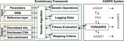
In the proposed framework depicted in Figure 4, the user provides the following information: (i) parameters controlling the run (Box 1), (ii) a DEM in raster grid file format (Box 2), and (iii) a reference layer (landscape attribute) in raster grid file format (Box 3). Parameters controlling the run include a list of acceptable CSA values, number of candidate solutions (population size), number of iterations (generations), percentage of crossover, percentage of mutation, and stopping criteria. In the initial iteration, the GA (Box 4) randomly generates a set of candidate solutions (population) in the form of a one-dimensional vector of floats and sends this information to the fitness module (Box 7), which converts each vector into two-dimensional arrays and applies the topographic parameterization algorithms (Box 9) to obtain a set of subdivided watersheds. Subdivided watersheds are individually discretized based on a majority voting procedure. The resulting discretized watershed is compared to the reference layer and a fitness score value is calculated. The set of fitness score values is sorted and genetic operations (Box 5) are performed on the candidate solutions with the top fitness score values (most fit individuals) to form the next set of candidate solutions (next population). Genetic operations considered include replication, crossover, and mutation. The new generation is then evaluated for fitness score calculation, and the entire process is repeated to form new populations with increasingly higher fitness score values until one of the stopping criteria is met (Box 8). To reduce computational overheads, the system was configured to perform the following DEM pre-processing steps prior to executing the evolutionary procedure: pit filling and reduction of small imperfections, flow direction, flow accumulation, local terrain slope, local terrain aspect, and other complementary topographic parameter calculations.

Once the evolutionary process concludes, the system produces: (i) a log file depicting a list of fitness scores for the most fit individuals throughout the evolutionary process – used to evaluate convergence; (ii) the candidate solution with the highest fitness score value – in one-dimensional vector format; and (iii) raster grid files containing the discretized sub-catchments (Box 9), CSA values in raster grid file format (Box 10), and the watershed sub-catchments and channel network in raster grid file format (Box 11). Inspection of fitness score values for all iterations (conversion) provides information on whether or not the optimal solution has been achieved.

Multi-objective design and convergence strategies

One important characteristic of the proposed framework is the two-objective optimization approach (Fig. 5). The first objective drives the evolutionary process to minimize the number of sub-catchments (Fig. 5(a)), while the second objective is designed to maximize the agreement between the discretized watershed and the user-provided reference GIS layer (Fig. 5(b)). Fitness score values from both objectives can be combined for graphical depiction of the evolutionary process (Fig. 5(c)).

Figure 5. Distribution of (a) number of sub-catchments, (b) kappa coefficient of agreement, and (c) combined fitness values for multiple generations (iterations) and individuals (candidate solutions). The multi-objective optimization methodology was devised to minimize the number of sub-catchments and to maximize the agreement between the discretized watershed and the reference dataset. These plots were generated using 10-m spatial resolution raster grids and soil type dataset as the reference layer.

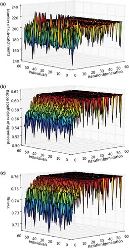
In this framework, the initial population is randomly generated. Individuals in this first set of candidate solutions often have poor fitness score values which iteratively increase as the evolutionary process advances. Additionally, there is a high level of fitness score value variance within population members. For instance, plotting the fitness score for the first objective illustrates the high variance in the number of sub-catchments during the earlier stages of the evolutionary process (Fig. 5(a)). Similar behavior can also be visualized for the second objective (Fig. 5(b)) and the combined fitness score value (Fig. 5(c)).

In these graphs, note the presence of individual candidate solutions with fitness score values significantly smaller than the remaining individuals within a generation, particularly towards the end of the evolutionary process. This “noise” is the result of mutation operations. The percentage of mutation was selected as the mechanism to control the overall diversity of the population: a key characteristic to assure genetic algorithms reach the global optimal solution rather than being trapped in a local sub-optimal solution.

Evaluation of the proposed system

Watershed description

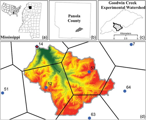
The proposed framework was evaluated through an application to a subset of the Goodwin Creek Experimental Watershed (GCW) located in Panola County, Mississippi, USA (Fig. 6). The GCW has been monitored by the US Department of Agriculture since 1982 for streamflow, sediment, farming practices, land use/land cover, and climate (Kuhnle et al. 1996). The GCW contains multiple streamgages and sediment sampling structures. Station 14 was selected as the drainage outlet for the determination of the basin used in this study (Fig. 6(c)). During the monitored period, land use/land cover consisted of crop agriculture, pasture, and forest; however, over the years, agricultural production has declined and row crop agriculture has been replaced by forest and pasture (Kuhnle et al. 2008). This site is located in the bluff hills region (just east of the flood plains of the Mississippi River), which is composed of silt loam soils; recognized as highly erodible soils when not protected by above-ground vegetation (Kuhnle et al. 1996). The main characteristic of precipitation events affecting soil erosion is isolated thunderstorms producing high intensity rainfall incidents. There were five precipitation gages that provided coverage of the spatial patterns of precipitation events within Station 14 (Fig. 6(d)). The average annual precipitation from these precipitation gages for 1982–1995 differed from each other by only 5%. The average annual precipitation at gages 14, 52, 53, 63, and 64 was 1399, 1353, 1346, 1342, and 1419 mm year⁻¹, respectively. Further information describing the physical watershed characteristics and the sediment sampling methods are provided in Kuhnle et al. (2008) and (1996), respectively.

Figure 6. (a) Study site located in southern USA, Mississippi State. (b) Site location in Panola County in (c) a subset of the Goodwin Creek Experimental Watershed. (d) Topography represented by DEM with 3-m spatial resolution; climate databases were created using information from five climate stations (dots), which were spatially assigned to sub-catchments based on their influence using the tessellation polygon method (dark polygons) and simulated runoff was compared to streamgage (star) information.

AnnAGNPS simulations

Changing how the physical watershed is internally represented as basic modeling units influences the AnnAGNPS estimations of surface flow and sediments. This was quantified through a relative comparison between multiple AnnAGNPS simulations where all the input parameters were held constant and only the watershed subdivision and, consequently, the watershed discretization for soils, management, and climate, was varied. A DEM generated from a LiDAR survey and resampled into a 3-m spatial resolution raster grid was used. The DEM was hydrologically corrected through manual removal of culverts and bridges for improved representation of surface water flow paths.

The application of AnnAGNPS to assess the impact of management practices has been demonstrated through various applications in the Conservation Effects Assessment Project (CEAP) and has been successfully used to accurately predict runoff and sediment in a variety of watersheds (Yuan et al. 2001, 2008, Baginska et al. 2003, Suttles et al. 2003, Licciardello et al. 2007). For example, AnnAGNPS-simulated monthly runoff and sediment were well correlated with observed values without calibration in Deep Hollow Lake watershed, located in Mississippi (R² = 0.9 for runoff on an event basis and 0.7 for monthly sediment; Yuan et al. 2001). AnnAGNPS has also been applied previously to the Goodwin Creek Watershed without calibration to estimate the effect of land use on sediment loads (Kuhnle et al. 1996, 1998). The application of AnnAGNPS for this study provides a tool that systemically integrates the most important processes that impact runoff and sediment load in a watershed, which is dependent on how the well the spatial variability of the watershed characteristics is described.

Watershed subdivision and sub-catchment discretization

Four reference GIS layers were used to evaluate the proposed framework: soil type (Fig. 7), landscape classification (Fig. 8), land use/land cover (farming management) (Fig. 9), and combined soil type and farming management (Fig. 10). Soil type layer was obtained from the NRCS database and clipped to the watershed boundaries. The landform classification layer consisted of segmenting the landscape hillslope position into five classes: summit, shoulder, backslope, footslope, and toeslope (Wysocki et al. 2000). This layer was generated using profile curvature, slope gradient, and relative elevation at different raster grid spatial resolutions and following the procedure proposed by Miller and Schetzl (2015). Farming management was developed based on annual land use/land cover unique rotations. A unique combination of yearly farming activities (crop types, irrigation, fertilization, and farming operations) for the entire simulation period was defined as a management practice. Farming management practices considered included different yearly rotations of forest, pasture, and row crops such as corn and soybeans. A total of 39 unique management practices were developed. Individual sub-catchments were assigned to a single management practice (Fig. 9(c)). Intersecting soil type with farming management formed the fourth reference layer (Fig. 10).

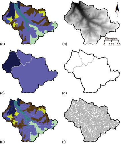
Figure 7. Utilization of spatially variable critical source area (a) to subdivide the watershed using topographic and soil type information (b) into 240 sub-catchments (c). The original soil type layer (b) can be compared to the soil type discretized watershed (d). A spatially constant critical source area of 0.1 ha was used to subdivide the watershed into 2170 sub-catchments (e), yielding the discretized soil type watershed (f).

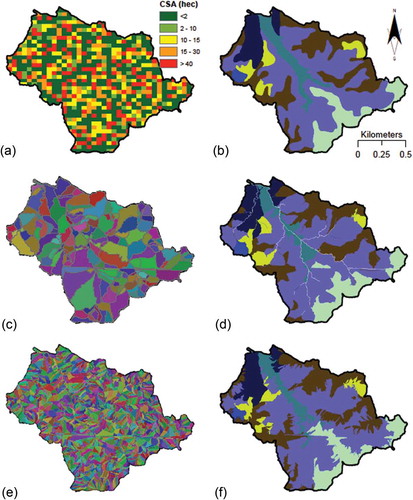
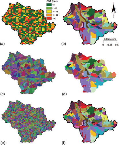
Figure 8. Utilization of spatially variable critical source area (a) to subdivide the watershed using topographic and landscape hillslope classification information (b) into 212 sub-catchments (c). The original hillslope classified layer (b) can be compared to the hillslope classification discretized watershed (d). A spatially constant critical source area of 0.1 ha was used to subdivide the watershed into 2170 sub-catchments (e), yielding the discretized landscape classification watershed (f).

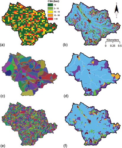
Figure 9. Utilization of spatially variable critical source area (a) to subdivide the watershed using topographic and farming management information (b) into 214 sub-catchments (c). The original management layer (b) can be compared to the management-discretized watershed (d). A spatially constant critical source area of 0.1 ha was used to subdivide the watershed into 2170 sub-catchments (e), yielding the discretized management watershed (f).

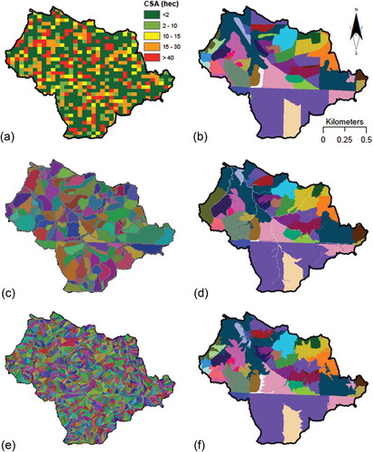
Figure 10. Utilization of spatially variable critical source area (a) to subdivide the watershed using topographic and merged soil type and management information (b) into 364 sub-catchments (c). The original reference layer (b) can be compared to the management/soil-discretized watershed (d). A spatially constant critical source area of 0.1 ha was used to subdivide the watershed into 2170 sub-catchments (e), yielding the discretized management watershed (f).

Multiple watershed subdivision scenarios were considered. One scenario consisted of a constant CSA value of 0.1 ha for the entire watershed (referred to herein as the constant scenario). This CSA value has been shown to be small enough to capture field sizes throughout the watershed and also closer in size to RUSLE experimental plot sizes. Additional scenarios were created using the proposed framework and the following reference layers: soil type, landscape hillslope classification, farming management, and intersection between soil type and farming management (referred to as merged).

A total of three realizations of the proposed framework for each scenario were executed and only the realization with the highest fitness value was recorded. This approach was adopted to minimize the influence of chance in the performance of the framework in developing the global optimal solution (Momm and Easson, 2010). Since the initial set of candidate solutions is randomly generated, it is possible that potential solution components are left out during the creation of the first population and, also, not included by mutation operations during the evolutionary process. When this occurs, the lack of important solution components in the genetic material set limits the convergence of the algorithm (algorithm arrives a local minimum rather than global minimum). All the parameters controlling the evolutionary process were the same for all realizations and all scenarios (Table 1). Finally, the watershed subdivision generated using the proposed framework was discretized using the remaining reference layers and a kappa coefficient of agreement calculated for each layer (Table 2).

Table 1. Parameters used to control genetic algorithm runs to evolve custom watershed subdivisions based on topography and landscape attributes.

Parameter	Value
Number of generations	150
Percentage of crossover	20%
Percentage of mutation	5%
CSA resampling factor	40
Population size	250
Weight for objective 1 (# sub-watersheds)	0.5, 1.0, 1.5
Weight for objective 2 (kappa statistics)	1.5, 1.0, 0.5
List of CSA possible values	40 values between 0.15–2.00 and 2.01–40.0

Table 2. Number of sub-catchments and kappa coefficient of agreement for scenarios with spatially varying CSA values derived using the integrated framework and the scenario with spatially constant CSA values.

				Kappa statistics
Reference layer	Weight Subwta	Weight kappa	Number of Subwta	Soil type	Landscape classification	Mngt	Merged
Soil type	0.5	1.5	240	0.62*	0.21	0.72	0.57
Landscape	1.5	0.5	212	0.56	0.24*	0.66	0.52
Management	0.5	1.5	214	0.59	0.19	0.75*	0.57
Merged	1.5	0.5	364	0.65	0.24	0.77	0.62*
Constant (0.1 ha)	n/a	n/a	2170	0.80	0.39	0.87	0.76

Subwta: sub-catchment; Mngt: farming management.

* Kappa statistic obtained from the evolutionary process.

Results and discussion

Streamflow and sediment load evaluation

The simulation period for all scenarios was 1982–1995 to match observed streamflow and sediment loads at the outlet. In this watershed, the main sources of suspended sediment at the outlet consisted of sheet and rill erosion (86%), with ephemeral gully and streambank erosion contributing the rest (Bingner 1998). A scenario was developed to include all sources of sediment for this period in a total load scenario including suspended and bedload material to compare the capabilities of AnnAGNPS to observed data. Simulations were performed without calibration as the AnnAGNPS parameters were determined with the best available information derived from field visits and expert knowledge of scientists working in the watershed for many years. In other watershed systems where effective values for model parameters are not available, calibration and validation of the simulation technology could provide for improved representation of local physical processes and add confidence to estimated values. The total amounts of annual streamflow at the outlet and at the end of the simulation period were 930 000 Mg year⁻¹ (estimated by AnnAGNPS) and 940 000 Mg year⁻¹ (observed). Similarly, the total sediment load simulated by AnnAGNPS was 2700 Mg year⁻¹, in comparison to observed total sediment load of 1860 Mg year⁻¹. The total fine sediment load simulated was 980 Mg year⁻¹ compared to 958 Mg year⁻¹ observed fine sediment load. The difference in observed and simulated total sediment loads is from the higher sand load produced by AnnAGNPS, which could be a result of the uncertainty of the sand to flow discharge relationships developed to produce observed sand values for every storm event (Kuhnle et al. 1996, 1998). In this study, to optimize the subdivision of the watershed, only sediment loads from sheet and rill sources were considered, as their sediment delivery estimation by existing modeling technology is very sensitive to how the watershed is subdivided and discretized.

Multiple AnnAGNPS simulations were performed where the only varying factor was the watershed subdivision and, consequently, the sub-catchments discretization and therefore the overall watershed characterization within the model under the homogeneity assumption (slope, CN, crop scheduling, soil properties, slope length, etc.). Simulated scenarios and observed annual streamflow at the outlet were compared (Fig. 11). Similarly, simulated and observed suspended sediment loads were compared (Fig. 12). The observed suspended sediment load represents the recording of suspended sediment from all erosional sources (sheet and rill, ephemeral gully, edge-of-field channel, streambank, etc.), while the simulated results constitute only estimates from sheet and rill erosion, particularly in agricultural fields. This limitation prevents a direct comparison between the observed and simulated, however, it is still possible to make assessments on the basis of temporal patterns between observed and simulated scenarios, and, more importantly, relative comparisons between each simulated scenario derived using the optimized framework (smaller number of sub-catchments) with the constant scenario (higher number of sub-catchments).

Sub-watershed discretization

During the pre-processing steps of AnnAGNPS input preparation efforts, each sub-catchment is discretized using multiple GIS layers representing different spatial landscape attributes. Using one layer as the input parameter into the optimized framework often yields a higher kappa coefficient of agreement for this particular layer than the alternatives discretized based on other layers (Table 2); for example, using the watershed subdivision obtained using topography and management layers as input to the optimized framework generated three discretized layers. The kappa statistic values obtained were 0.75, 0.72, and 0.66 for this particular watershed subdivision when discretized for farming management, soil type, and landscape form classification, respectively. These values indicate the customization of the watershed subdivision to the user-defined reference layer; in this example farming management. However, using as reference layer the intersection between management and soil type yielded higher agreements between the reference layer and the discretized sub-catchments at the cost of a higher number of sub-catchments: 364 compared to 214, 212, and 240 of the other scenarios.

Spatially variable CSA values, defined by the optimized framework, represented appropriately the spatial variation of soil type (Fig. 7), landscape hillslope classification (Fig. 8), farming management (Fig. 9), and merged soil type and farming management (Fig. 10). The final optimization-defined discretized reference layers were comparable to the respective discretized layers obtained with a watershed subdivision generated using a spatially constant CSA value but with a significantly higher number of sub-catchments. Each watershed discretized with the optimized framework was compared to the original reference layer. This comparison used the kappa coefficient of agreement to quantify the agreement between pairs of discretized watersheds represented as raster grid layers (calculations used all raster grid cells within watershed boundaries). The kappa coefficients of agreement calculated and number of sub-catchments obtained were 0.62/240, 0.24/212, 0.75/214, and 0.62/364 for each reference layer soil type, landscape hillslope classification, management, and merged soil type and management, respectively (Figs 7(d), 8(d), 9(d), and 10(d)). A watershed discretized using a spatially constant critical source area of 0.1 ha yielded 2170 sub-catchments (Figs 7(e), 8(e), 9(e), and 10(e)). Similar comparison between the discretized watershed using a constant CSA value and the reference layers produced kappa coefficient of agreement values of 0.79, 0.39, 0.87, and 0.76 for each reference layer soil type, landscape hillslope classification, management, and merged soil type and management, respectively (Figs 7(f), 8(f), 9(f), and 10(f)).

The scenario depicting the use of landscape form classification as the reference layer output the least agreement (Fig. 8). In this scenario, the lower agreement values can be attributed to the small scale on which landform classes varied spatially compounded with one landscape class occurring significantly more than others (light blue class in Fig. 8(c)); therefore shedding light on the existence of a potential lower bound limit of scale on which the homogeneity assumption needs to be re-evaluated. While landscape classification is not needed for AnnAGNPS simulations, this can be used to better represent watersheds with multiple topographic patterns.

Streamflow and sediment yield

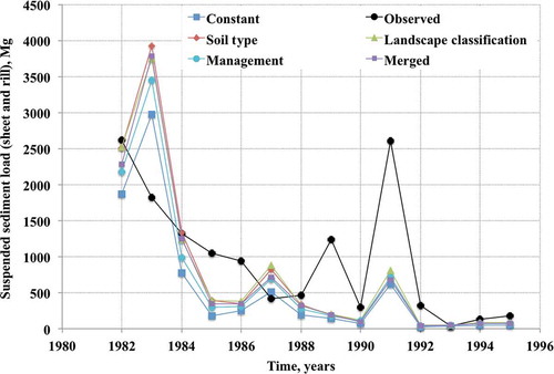
Similarly to documented studies, the level of watershed subdivision had a limited effect on the streamflow estimates at the outlet (Fig. 11). The relative trend of simulated and observed annual runoff matched the trends of annual precipitation, but with limited variability of runoff between scenarios. Conversely, varying watershed subdivision impacted the estimation of sediment loads. Studies have demonstrated a positive correlation between the average sub-catchment area and the annual average sediment yield (Arabi et al. 2006, Parker 2009, Pradhanang and Briggs 2013). However, the watershed subdivision impacted the estimation of sediment loads from sheet and rill erosion disproportionally, even among scenarios with a similar number of sub-catchments (Fig. 12). All of the scenarios demonstrated the same overall pattern. However, the scenario using farming management was significantly closer to the scenario generated using the constant CSA value, even closer than the scenario representing merged soil type and farming management. The overestimation of suspended sediment for 1983 could be a result of the significant amount of runoff from over 300 mm of precipitation from the event of 21 September 1983. The observed runoff could have overwhelmed the capability of the gage to allow accurate observations of the runoff and sediment from this event. Simulated runoff from this event was 200 000 m³ higher than observed and suspended sediment was over 1200 Mg higher than observed.

Figure 11. Observed and simulated annual streamflow at the outlet along with recorded total precipitation at the watershed. Different simulated curves were generated using varying watershed subdivisions using the optimized framework and distinct reference landscape attribute layers.

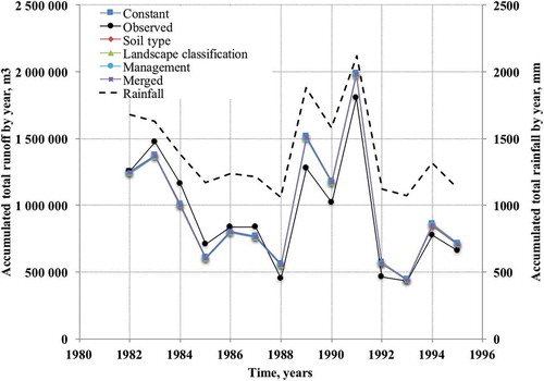
Figure 12. Observed and simulated suspended sediment load. Observed values represent values from all sources of sediment while simulated are from sheet and rill only. Different simulated curves were generated using varying watershed subdivisions using the optimized framework and distinct reference landscape attribute layers.

The effect of the watershed subdivision can be also evaluated through comparison of the ranked land area within the watershed and the estimated sediment contribution of each sub-catchment (Fig. 13). For instance, 40% of the watershed total area was shown by the simulation to produce 83% (landscape form classification and soil type), 86% (merged) and 89% (farming management and constant CSA value) of sediments delivered from sheet and rill erosion sources to the outlet. The identification of these critical areas (covering 40% of the watershed) supports the optimal allocation of limited resources that maximizes the reduction in sediment delivery. Furthermore, farming management and constant scenarios agree that 40% drainage area produces 89% of suspended sediment loads. However, the scenario developed using farming management represents 40% of the watershed drainage area with 75 sub-catchments, while the scenario using a constant CSA value represents the same area with 790 sub-catchments. This can be attributed to the significant effect of land use/land cover on the model’s ability to estimate daily variations in water balance (soil moisture, evapotranspiration, etc.) properties and curve number. Over-subdivision of the watershed tends to convert field slope lengths into defined channels and therefore transforming the model representation of laminar flow lengths, which are associated with sheet and rill erosion, into channel erosion processes (ephemeral gullies and streambank). Essentially, more sub-watersheds result in smaller LS-factor values for each sub-watershed used in the RUSLE calculation of sheet and rill erosion amounts, accompanied by additional reaches resulting in more channel erosion estimation (Pradhanang and Briggs 2013).

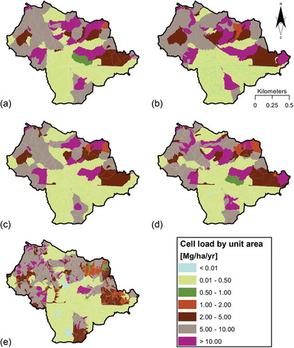
Comparisons of spatial patterns for suspended sediment loads per unit of area indicate agreement between all the scenarios considered (Fig. 14(a)–(d)) and the constant scenario (Fig. 14(e)). Comparison of AnnAGNPS simulation results of individual raster grid cells reveals, on average, a small underestimation of sediment loads (<1.5 Mg ha⁻¹ year⁻¹) between the optimized scenarios and the scenario generated using a spatially constant CSA of 0.1 ha, designated as the reference layer (Table 3), particularly between the optimized subdivision using management as reference layer (Fig. 14(c)). Although, it has been described in the literature that the selection of appropriate sub-catchment sizes is critical to proper estimation of sediment yield (Bingner et al. 1996, FitzHugh and Mackay 2000); this spatial agreement signifies an appropriate characterization of key parameters important for watershed models. The optimized “trial-and-error” fashion of the evolutionary algorithms selected the smallest number of spatially varying sub-catchment sizes that still “captured” the watershed land cover characteristics important for sediment yield estimation.

Table 3. Comparison of AnnAGNPS simulation results between watershed characterization using optimized watershed subdivision and watershed subdivision using constant CSA.

Dataset	Differences in sediment load per unit of area		Fitting linear model between optimized/distributed and constant CSA scenarios
	SD	Mean	Slope	Intercept	r value	p value	Standard error
Soil type	3.567	–1.419	0.897	1.772	0.700	<0.001	0.0022
Landform	3.982	–1.404	0.824	2.007	0.631	<0.001	0.0024
Management	3.343	–0.755	0.871	1.196	0.714	<0.001	0.0020
Merged	3.176	–1.118	0.991	1.148	0.770	<0.001	0.0019

SD: standard deviation.

Figure 13. Individual sub-catchment sediment load contribution by ranked unit area drainage area.

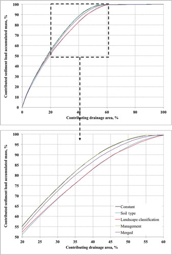
Figure 14. Spatial distribution of sediment load per unit of area for different watershed subdivisions generated with the optimized framework using different reference layers: (a) soil type, (b) landscape form classification, (c) farming management, and (d) merged soil type and farming management. (e) These layers are compared with a watershed subdivision generated using a spatially constant CSA of 0.1 ha.

Conclusions

A qualitative trial-and-error approach is commonly used to define the watershed subdivision used in hydrological simulation models. A small number of topographic threshold values are typically tested one at a time to generate a discretized watershed and visually compared with landscape attributes for watershed simulations. In the majority of these cases, a single constant threshold value is considered for the entire watershed.

In this study, a methodology is proposed to quantitatively determine the set of spatially variable threshold values using two landscape attributes: topography and another user-defined reference layer, such as soil type, farming management, landscape hillslope classification, and combinations of these layers. An optimization algorithm was integrated with topographic parameterization to evolve solutions to meet two objectives: minimize the number of watershed subdivisions and maximize the agreement between the discretized watershed and the reference layer.

Using the integrated framework to define the optimal watershed subdivision and discretization, some reference layers were found to be more significant than others when evaluating estimated sediment loads from AnnAGNPS. The scenario in which the watershed was subdivided using farming management as the reference layer yielded closer results to the scenario with approximately 10 times more sub-catchments.

Future investigations should be conducted to determine and quantify the lower-bound scale at which the homogeneity assumption does not hold. As seen with the scenario using the landscape classification reference layer, variations of a few raster grid cells in size were ignored by the discretization procedure. The size of the study site can also be a concern for future investigation, but the optimal framework described should be independent of scale, as the impact of the spatial variability of the associated soil, land use and climate characterizations would have the greatest impact compared to scale.

Watershed modeling and simulation technology has been recognized as a critical tool needed to support sustainable watershed management planning through timely and cost-effective allocation of resources and implementation of conservation practices. The quality and applicability of this technology depends on accurately representing and describing physical processes. This starts with appropriate characterization of watershed properties through a subdivision of the watershed into modeling basic spatial units and their suitable discretization.

Acknowledgments

We would like to thank Glenn Herring for his support in the integration of topographic parameterization algorithms with evolutionary computation technology. The authors also acknowledge NASA-Tennessee Space Grant Consortium for providing graduate student support.

Disclosure statement

No potential conflict of interest was reported by the authors.

References

- Arabi, M., et al., 2006. Role of watershed subdivision on modeling the effectiveness of best management practices with SWAT. Journal of the American Water Resources Association, 42, 513–528. doi:10.1111/jawr.2006.42.issue-2
- Baginska, B., Milne-Home, W., and Cornish, P.S., 2003. Modeling nutrient transport in currency Creek, NSW with AnnAGNPS and PEST. Environment Model Softw, 18 (8), 801–808. doi:10.1016/S1364-8152(03)00079-3
- Bingner, R.L., 1998. Systems analysis of runoff and sediment yield from a watershed using a simulation model. Thesis (PhD). Urbana, IL: University of Illinois, 305.
- Bingner, R.L., et al., 1996. Effect of watershed subdivision on simulation runoff and fine sediment yield. Transactions of the ASAE, 40 (5), 1329–1335. doi:10.13031/2013.21391
- Bingner, R.L. and Theurer, F.D., 2001. AGNPS 98: a suite of water quality models for watershed use. In: Proceedings of the Sedimentation: Monitoring, Modeling, and Managing, 7th Federal Interagency Sedimentation Conference, Reno, NV, 25–29 Mar. 2001 Washington, DC: United States Dept. of the Interior, Bureau of Land Management, p. VII-1–VII-8.
- Bingner, R.L., Theurer, F.D., and Yuan, Y., 2015. AnnAGNPS Technical Processes, Unpublished Report, USDA-ARS National Sedimentation Laboratory: Oxford, MS. Available from: http://www.wcc.nrcs.usda.gov/ftpref/wntsc/H&H/AGNPS/downloads/AnnAGNPS_Technical_Documentation.pdf [ Accessed March 2015].
- Chiang, L.C. and Yuan, Y., 2015. The NHDPlus dataset, watershed subdivision and SWAT model performance. Hydrological Sciences Journal, 60 (10), 1690–1708. doi:10.1080/02626667.2014.916408
- Cohen, J., 1960. A coefficient of agreement for nominal scales. Educational and Psychological Measurement, 20 (1), 37–46. doi:10.1177/001316446002000104
- Cronshey, R.G. and Theurer, F.D., 1998. AnnAGNPS: non-point pollutant loading model. In: 1st Federal Interagency Hydrologic Modeling Conference. Las Vegas, NV: U.S. Interagency Advisory Committee on Water Data, 1, 1-9–1-16.
- FitzHugh, T.W. and Mackay, D.S., 2000. Impacts of input parameter spatial aggregation on an agricultural nonpoint source pollution model. Journal of Hydrology, 236, 35–53. doi:10.1016/S0022-1694(00)00276-6
- FitzHugh, T.W. and Mackay, D.S., 2001. Impact of subwatershed partitioning on modeled source- and transport-limited agricultural nonpoint source pollution model. Journal of Soil Water Conservation, 56 (2), 137–143.
- Fogel, D.B., 2000. Evolutionary computation: toward a new philosophy of machine learning. New York, NY: IEEE Press.
- Garbrecht, J. and Martz, L., 1996. Digital landscape parameterization for hydrological applications. In: HydroGIS 96: application of Geographic Information Systems in Hydrology and Water Resources Management (Proceedings of the Vienna Conference, April). IAHS Publ. no. 235, 169–174.
- Garbrecht, J.D., Campbell, J., and Martz, L.W., 2004. TOPAZ user manual-updated manual. El Reno, OK: Grazinglands Research Laboratory Miscellaneous Publication No. GRL 04-3. 169.
- Jenness, J. and Wynne, J.J., 2004. Cohen’s kappa and classification table derived metrics: an ArcView 3x extension for the accuracy assessment of spatial-explicit models. http://www.jennessent.com/arcview/kappa_stats.htm [ Accessed April 2015].
- Jha, M., et al., 2004. Effect of watershed subdivisions on SWAT flow, sediment, and nutrient predictions. Journal of the American Water Association, 40 (3), 811–825. doi:10.1111/j.1752-1688.2004.tb04460.x
- Kalin, L., Govindaraju, R.S., and Hantush, M.M., 2003. Effect of geomorphological resolution on modeling of Runoff Hydrograph and sedimentograph over small watersheds. Journal of Hydrology, 276, 89–111. doi:10.1016/S0022-1694(03)00072-6
- Koza, J.R., 1992. Genetic Programming: on the programming of computers by means of natural selection. Cambridge, MA: MIT Press.
- Kuhnle, R.A., et al., 2008. Conservation practice effects on sediment load in the Goodwin Creek Experimental Watershed. Journal of Soil and Water Conservation, 63, 496–503. doi:10.2489/jswc.63.6.496
- Kuhnle, R.A., et al., 1996. Effect of land use changes on sediment transport in Goodwin Creek. Water Resources Research, 32 (10), 3189–3196. doi:10.1029/96WR02104
- Kuhnle, R.A., et al., 1998. Chapter 13 - Land use changes and sediment transport on Goodwin Creek. In: P.C. Klingeman, et al., eds. Gravel-Bed rivers in the environment. Highlands Ranch, CO: Water Resources Publications, LLC, 279–292.
- Licciardello, F., et al., 2007. Runoff and soil erosion evaluation by the AnnAGNPS model in a small Mediterranean watershed. Transactions of ASABE, 50 (5), 1585–1593. doi:10.13031/2013.23972
- Miller, B.A. and Schetzl, R.J., 2015. Digital classification of Hillslope Position. Soil Science Society of America Journal, 79, 132–145. doi:10.2136/sssaj2014.07.0287
- Momm, H.G., et al., 2011b. AGNPS GIS-based tool for watershed-scale identification and mapping of cropland potential ephemeral gullies. Applied Engineering in Agriculture, 28 (1), 1–13.
- Momm, H.G., et al., 2016. Characterization and placement of wetlands for integrated conservation practice planning. Transactions of the ASABE, 59 (5), 1345–1357. doi:10.13031/trans.59.11635
- Momm, H.G., et al., 2014. Spatial characterization of riparian buffer effects on sediment loads from watershed systems. Journal of Environmental Quality, 43 (5), 1736–1753. doi:10.2134/jeq2013.10.0413
- Momm, H.G. and Easson, G.L., 2010. Population restarting: a study case of feature extraction from remotely sensed imagery using textural information. In: The 12th Annual Conference on Genetic and Evolutionary Computation, July 7–11, Portland, OR.
- Momm, H.G., Easson, G.L., and Bingner, R.L., 2011. Evaluation of the use of remotely sensed evapotranspiration estimates into AnnAGNPS pollution model. Ecohydrology, 4, 650–660. doi:10.1002/eco.155
- Nour, M.H., et al., 2007. Effect of watershed subdivision on water-phase phosphorus modeling: an artificial neural network modeling application. Journal of Environmental Engineering Science, 7, S95–S108. doi:10.1139/S08-043
- Parker, G., 2009. Uncertainty metrics for coupled watershed models. Thesis (PhD). Ottawa, Canada: Department of Civil Engineering at University of Ottawa.
- Parker, G.T., Rennie, C.D., and Droste, R.L., 2011. Model structure and uncertainty for stochastic non-point source modeling applications. Hydrological Sciences Journal, 55 (5), 870–882. doi:10.1080/02626667.2011.586350
- Pradhanang, S.M. and Briggs, R.D., 2013. Effects of critical source area on sediment yield and streamflow. Water and Environmental Journal, 28, 222–232. doi:10.1111/wej.12028
- Renard, K.G., 1997. Predicting soil erosion by water: a guide to conservation planning with the revised universal soil loss equation (RUSLE). Agriculture Handbook Number 703. USDA: Washington, DC.
- Rouhani, R., Feyen, J., and Willems, P., 2006. Impact of watershed delineation on the SWAT runoff prediction: a case study in the Grote Nete catchment, Flanders, Belgium. In:Proceedings of the 2006 IASME/WSEAS int. Conf. on Water Resources, Hydraulics and Hydrology, Chalkida, May 11–13, Greece.
- Suttles, J.B., et al., 2003. Watershed-scale simulation of sediment and nutrient loads in Georgia Coastal Plain streams using the Annualized AGNPS model. Transactions of ASAE, 46 (5), 1325–1335. doi:10.13031/2013.15443
- Theurer, F.D. and Clarke, C.D., 1991. Wash load component for sediment yield modeling. In: 5th Federal Interagency Sedimentation Conference, Washington, DC: Interagency Advisory Committee on Water Data, Subcommittee on Sedimentation, Vol. 1: 7–1 –7–8.
- Tripathi, M.P., Raghuwanshi, N.S., and Rao, G.P., 2006. Effect of watershed subdivision on simulation of water balance components. Hydrological Processes, 20, 1137–1156. doi:10.1002/(ISSN)1099-1085
- USDA-SCS, 1972. National engineering handbook. Section 4: hydrology. Washington, DC: US Government Printing Office.
- Wales, P.M., 2005. Quantitative Analysis of Land Loss in Coastal Louisiana Using Remote Sensing. Thesis (Master). University, MS: University of Mississippi.
- Wang, X. and Lin, Q., 2011. Impact of critical source area on AnnAGNPS simulation. Water Science and Technology, 64 (9), 1767–1773. doi:10.2166/wst.2011.641
- Wysocki, D.A., Schoeneberger, P.J., and LaGarry, H.E., 2000. Geomorphology of soil landscapes. In: M.E. Sumner, editor. Handbook of soil science. Boca Raton, FL: CRC Press, E5–E40.
- Yuan, Y., Bingner, R.L., and Rebich, R.A., 2001. Evaluation of AnnAGNPS on Mississippi delta MSEA watersheds. Transactions of ASAE, 45 (5), 1183–1190.
- Yuan, Y., Locke, M.A., and Bingner, R.L., 2008. Annualized agricultural non-point source model application for Mississippi delta Beasley Lake watershed conservation practices assessment. Journal of Soil and Water Conservation, 63 (6), 542–551. doi:10.2489/jswc.63.6.542
- Zema, D.A., et al., 2012. Evaluation of runoff, peak flow and sediment yield for events simulated by the AnnAGNPS model in a Belgian agricultural watershed. Land Degradation and Development, 23, 205–215. doi:10.1002/ldr.1068