Extracting water-related features using reflectance data and principal component analysis of Landsat images

ABSTRACT

This study aimed to map water features using a Landsat image rather than traditional land cover. We involved the original bands, spectral indices and principal components (PCs) of a principal component analysis (PCA) as input data, and performed random forest (RF) and support vector machine (SVM) classification with water, saturated soil and non-water categories. The aim was to compare the efficiency of the results based on various input data. Original bands provided 93% overall accuracy (OA) and bands 4–5–7 were the most informative in this analysis. Except for MNDWI (modified normalized differenced water index, with 98% OA), the performance of all water indices was between 60 and 70% (OA). The PCA-based approach conducted on the original bands resulted in the most accurate identification of all classes (with only 1% error in the case of water bodies). We therefore show that both water bodies and saturated soils can be identified successfully using this approach.

KEYWORDS:

• multivariate analysis
• principal component analysis
• remote sensing
• Landsat
• classification uncertainty analysis
• spectral index

Editor A. Castellarin Associate editor F. Tauro

1 Introduction

Monitoring phenomena on the surface of the Earth is important in scientific research and decision making; in this context, remote sensing (RS) techniques are an effective tool to accomplish these tasks (Sawaya et al. 2003, Wallace et al. 2009). RS is widely used in landscape assessment to identify vegetation (even at the species level) over large areas, impervious surfaces, or water bodies (Xu 2005, Weng 2012, Li et al. 2013, Lu et al. 2014, Burai et al. 2015). Detecting surface water resources and saturated soil, and exploring how they change over time, is one of the most important issues related to future climate change (Vörösmarty et al. 2000, Barnett et al. 2004). Thus, soil moisture mapping plays an important role in operational drought management. One basis for predicting required regional water resources is the determination of the spatial distribution of the moisture stored in soil (Narasimhan and Srinivasan 2005). Organizations responsible for water resource management increasingly demand accurate RS data calibrated by ground measurements; therefore, in addition to the lack of water resources, surplus water mapping is also important (van Leeuwen et al. 2012). Nowadays, in many cases, the determination of the spatial extent of floods is performed based on ground observations, which are unsuitable for surveying saturated soils; but, because water can be identified with a high degree of accuracy using spectra due to their low reflectance rate above 700 nm, unique to this electromagnetic range (Schowengerdt 2007), flood mapping based on RS is appropriate to measure the extent of saturated areas as well as levels. Soils with maximum water capacity cause similar damage to agriculture as do floods; thus, water regime investigations based on accurate soil moisture measurements also can play an important role in describing runoff processes in hilly areas (Melesse and Shih 2002). The development of flash floods strongly depends on infiltration processes, which are themselves influenced by initial soil moisture content early phases (Hegedüs et al. 2015).

As a method, RS can be either passive (utilizing optical sensors) or active (utilizing radar or laser sensors). However, although radar-based RS has fewer limiting factors (e.g. images that are independent of cloud cover) and has been applied several times to water-related questions (Alsdorf et al. 2000, Di Baldassarre et al. 2009), we utilize just satellite images captured with optical sensors in this study because of their wide range of applications to land-cover mapping and because they can be interpreted and processed in several ways. Optical RS images can be interpreted using mathematical algorithms based on the different spectral characteristics of surface features and materials (Srivastava et al. 2012); one approach often used in land-cover classification is supervised or unsupervised classification of spectral bands (Lu and Weng 2007). Supervised classification requires preliminary knowledge of the area, however; i.e. to train algorithms to identify objects we need to classify them with the outcomes of this process comprising the classes we define (e.g. a forest, grassland, or water body). In contrast, unsupervised classifications are based on cluster analysis and use only the spectral information of the images; thus, the outcomes of this approach are spectral classes that can encompass the objects we try to extract. Supervised classification methods are therefore more reliable because of their thematic accuracy (Schowengerdt 2007, Sonka et al. 2014). One common and efficient type of classification that is often applied in this context is the maximum likelihood classifier (MLC), but newer methods, such as random forest (RF) or support vector machine (SVM), can also perform tasks with high efficiency (Jin et al. 2005, Otukei and Blaschke 2010).

Additional available image processing techniques are based on band ratios and use thresholds that indicate a phenomenon (e.g. biomass or water), usually as an index value derived from two or more bands (Singh 1989). Spectral indices are therefore often calculated with a red and a near-infrared band, enhancing the differences in the land-cover types with the aim of more accurately distinguishing them (Demetriades-Shah et al. 1990); vegetation indices (VI) are widely used to provide information about biomass (Liu et al. 2012, Marshall and Thenkabail 2015, Aly et al. 2016), and water indices (WIs) are also often applied in Earth systems research (Estoque and Murayama 2015, Kumar 2015).

Satellite bands and spectral indices usually correlate with one another and thus bias classification results. One common technique applied to mitigate this is a multivariate approach applying an ordination (dimension reduction), the use of fewer artificial non-correlating variables (factors or principal components; PCs) instead of the numerous original variables to enable total variance to be retained at a high level. Principal component analysis (PCA) is one ordination method that is frequently used to reduce multidimensional datasets (Eklundh and Singh 1993, Munyati 2004, Deng et al. 2008). Classifications using this approach can be performed on original bands, spectral indices or PCs.

The aim of satellite image classification is usually to delineate land-cover maps, but encapsulated spectral information can also be used to identify other features. Thus, the hypothesis tested in this paper is that water and water-related objects on the surface (such as saturated soils or vegetation under wet conditions) can also be identified using these images. Previous studies in this area have focused on the relationship between WIs and environmental factors (e.g. urban heat islands or soil moisture content; Chen et al. 2006, Gu et al. 2008) or their aims were restricted to the identification of water bodies (Ko et al. 2015). Although the performance of supervised classifications for water-related objects has not yet been quantified, it is nevertheless important to determine how accurately WIs can provide information on water bodies and wet surfaces even though their thematic accuracy remains unclear; in other words, where is the boundary between a water body and a wetland, and do the highest values in these classifications actually reflect water bodies? Image classification combined with accuracy assessment is one approach to these questions.

The image-acquisition satellite Landsat 7 was operational for 17 years (1999–2016) and provided a huge amount of data that was used for environmental monitoring. The aim of this study was therefore to utilize this dataset and to reveal its potential for water-related topics because of their relevance to climate change issues. We therefore test the efficiency of spectral indices and evaluate a PCA-based approach vs a traditional, satellite band-based technique for the identification of water bodies, saturated soils/vegetation under wet conditions, and non-water-related classes. We also evaluate the accuracy of WI efficiency in this study. Our hypothesis is that the use of uncorrelated PCs provides enhanced classification results compared to the use of original bands. We also summarize the advantages of different indices and explore their inter-relationships.

2 Materials and methods

2.1 Study area

The study area comprised the Rétköz micro-region (Fig. 1) in northeastern Hungary, a region (275 km²) that is regularly at risk of inundations of excess water and flooding. The area can be divided into two main zones according to their genetic and geomorphological characteristics: (a) the western part, with alluvial forms and soils with a high clay content, which leads to surface-layer impermeability; and (b) the eastern part, where eolic accumulations dominate and soils have a high sand content (Pásztor et al. 2016).

Figure 1. Location of the study area.

One common phenomenon in Hungary is the formation of surface water due to pluvial floods. These water bodies only form in plain areas, however, where runoff and infiltration is limited by topography and soils have a high clay content. Such surface water accumulations can have different extents (from 10–20 m² to hundreds of hectares) and persist for a number of weeks, but soils remain saturated for longer times, which causes problems for agriculture in ploughed lands as machine cultivation can be impossible at the start of the vegetation period and yields are weak (Kuti et al. 2006). The western part of the study area contains substantial regions that are endangered by this type of surface water, especially in the spring when the snow melts and precipitation is high (Pásztor et al. 2015). In contrast, the eastern part of the study region remains rather dry due to the high infiltration rate of the sandy soil. It is noteworthy that, because the Landsat images applied in this work do not cover the whole micro-region, results were interpreted based on the section that was covered.

2.2 Dataset and derived WIs

We used a LANDSAT 7 ETM+ (radiometrically and atmospherically corrected) image in this research, which was acquired on 23 April 2000. During the period 10 March–12 May 2000, a large flood wave had inundated the floodplain of the Tisza River and a relatively high proportion of this area was under water (Water Quality Report 2000).

We calculated nine spectral indices from Landsat image bands (Table 1), all developed to enhance the pixel intensity of those parts where the water component could be found, and to aid their identification. As these indices perform differently in this task; our aim was to identify the most effective.

Table 1. Derived spectral indices (B2: green band; B3: red band; B4: near-infrared band; B5: shortwave infrared band of the Landsat 7 image).

Index	Landsat band	Authors
AVI: Ashburn vegetation index	2B4 − B3	Ashburn (1979)
NDVI: normalized difference vegetation index	B4 − B3/B4 + B3	Rouse et al. (1974)
RVI: ratio vegetation index	B3/B4	Richardson and Wiegand (1977)
NRVI: normalized ratio vegetation index	RVI − 1/RVI + 1	Baret and Guyot (1991)
TVI: transformed vegetation index		Deering et al. (1975)
CTVI: corrected transformed vegetation index		Perry and Lautenschlager (1984)
TTVI: Thiam’s transformed vegetation index		Thiam (1997)
NDWI: normalized difference water index	B4 − B2/B4 + B2	McFeeters (1996)
NDWI: normalized difference water index	B5 − B4/B5 + B4	Gao (1996)
MNDWI: modified normalized difference water index	B5 − B2/B5 + B2	Xu (2006)

2.3 Principal component analysis (PCA) of original satellite bands and WIs

We utilized a standardized PCA with Varimax rotation in this study in order to reduce multi-dimensionality and to reveal correlations among variables, i.e. nine WIs or six TM bands (Davis 1986, Meglen 1992). We also applied a log(k_i + 1) transformation, where k_i is the ith element of the dataset, to improve the linearity and normal distribution of the variables (van den Berg et al. 2006). Thus, based on common features, we preserved all the variables in the PCA model and, according to Kaiser’s rule, extracted PCs with an eigenvalue greater than one (Jolliffe 2002). We then tested the classification performance of original bands and WIs separately to highlight the efficiency of the traditional approach and potential band ratio usage, performed a PCA on the training dataset, and plotted the results on a bi-plot diagram, which revealed the data distribution in ordination (multivariate) space as well as the variances and the correlations of the variables (Gabriel 1971, Kohler and Luniak 2005). Bi-plots are valuable tools to illustrate the discrimination of data points on the basis of pre-defined categories in multivariate space: if data points of different categories intersperse then classifications cannot be successful using the PCs, while if points occur in well-defined clusters (along 95% ellipses or convex hulls), this method provides a favourable classification.

We tested model fit using root mean square residuals (RMSR; Jöreskug and Sörbom 1996) calculated from the residuals of the correlation matrix determined from the original dataset and the PCA model estimation (Equation (1)), in addition to the adjusted goodness-of-fit index (AGFI; Jaccard and Wan 1996, Jöreskug and Sörbom 1996) (Equation (2)). Thus, RMSR values that are below 0.1 are considered good, while those below 0.05 reflect a very good fit; similarly, AGFI are indicative of a good fit if a recovered value is more than 0.9 and very good if above 0.95 (Basto and Pereira 2012). Our PCA led to generation of a new set of PC images.

(1)

(2)

where p + q refers to the number of observed variables, s_ij is the observed covariance, σ_ij is the reproduced covariances, d denotes the degree of freedom in the model, F₀ is the fit function when all parameters in the model are zero, and F_ML is the maximum likelihood estimation.

All PCAs in this study were performed using the software R 3.3 (R Core Team 2016) by applying the psych (Revelle 2015) and GPArotation packages (Bernaards and Jennrich 2005), while bi-plots were generated using the factoextra and FactoMineR packages (Lê et al. 2008, Kassambara and Mundt 2017).

2.4 Image classification

We utilized two classifier algorithms in this study, RF and SVM, to reveal the efficiency of different approaches, and distinguished three water-related classes: water bodies, saturated soils/vegetation under wet conditions (referred to as saturated soils), and non-water. Classifications were conducted using original bands as in the traditional approach, including the use of spectral indices (separately, and in different combinations), and utilizing a PCA-based image classification approach (Fig. 2).

Figure 2. Flowchart of the classification process.

The RF method is a modern machine learning technique that is based on decision trees (Ho 1995, Pal 2005). Thus, a large number of decision trees (in our case 500) were incorporated with different, randomly selected data and variables (i.e. spectral indices or Landsat TM bands). This means that the number of variables involved is the square root of all variables; in all cases these were chosen randomly in a single decision tree, and the procedure was repeated 500 times. Our final dataset used 500 independent classifications with different thematic accuracies; based on the effect of omitting a variable, this method is, however, able to rank the importance of those involved, which means that we were able to quantify the effect of dropping one given variable, so-called mean decrease accuracy (MDA; Breiman 2001, Louppe et al. 2013). The advantage of the method is that there is no prerequisite for normal distribution or homoscedasticity.

The alternative SVM method is another modern and robust approach for classification based on the search for optimal hyperplanes that maximize the margin of data points belonging to different classes (Vapnik 1995). In other words, this algorithm seeks the largest distance from the nearest data point of any class; therefore, the larger the distance, the smaller the generalization error (classification accuracy using data other than the training dataset; Mukherjee et al. 2006). Usually, datasets cannot be separated linearly, but due to further algorithm developments this approach can also cope with nonlinear data (Amari and Wu 1999). Data were transformed into a higher dimensional space, which enables easier separation; in these cases, data points were replaced with kernel functions, and a maximum-margin hyperplane fit was conducted in a so-called transformed feature space where an n-dimensional vector of numerical features represents the same objects. The method is independent of the number of dimensions because in feature space the input is the distance between the data points. We therefore applied the radial basis function, where parameters are determined automatically to minimize the upper limit of the expected test error (Schölkopf et al. 1997) when applying this approach. Both RF and SVM classifications were performed using the rattle package in the software R 3.3 (Williams 2011), and images were produced using the software Idrisi Selva (Clark Labs 2012).

We developed a training and a testing dataset for this study, taking water surfaces and the saturation state of soils into consideration (i.e. 1702, 292 and 426 pixels for non-water, saturated soils and water, respectively, in proportion to their dominance in the study area). The dataset was split 70:30 between training and testing for further analyses.

We reported thematic accuracy using a cross-tabulation matrix, where columns represent the reference data and rows denote classified (modelled) ones. Thus, based on this table, we report overall accuracy (OA) and producer’s accuracy (PA). In this case, OA represents the diagonal fields in which classified and reference pixels are the same (i.e. the model was accurate); this value is a general expression of percentage accuracy, while PA is the omission error when we summarize the accurate pixels and take into account misclassifications at the class level. As these values show how accurate the maps are for each class (Congalton 1991), we were able to evaluate the advantages and disadvantages of each classification in this study.

Similarly, ground truth data were collected with the help of thematic maps of surface water formed by pluvial floods (and soils with poor permeability) surveyed by the water management directorates each year, and we also used aerial images. The thematic maps used in this study contained surface water patches that encompassed a different extent each year, depending on the amount and distribution of melting snow and precipitation. We used these maps as auxiliary data to limit the area where surface water can occur and delineated just those pixels as a “water body” or “saturated soil” when discrimination was also obvious on satellite images. However, even though aerial images are usually not captured at the right time of year to be useful for mapping water features, these images nevertheless contain trait-based information which can be extracted via visual interpretation. Accordingly, we identified direct (e.g. water bodies or dark soil patches indicating saturation) and indirect (i.e. deviances in patch texture such as a dark/light patch within a larger patch) traits. We assembled a dataset of 2420 pixels (1702, 292 and 426 pixels for non-water, saturated soil and water, respectively, all proportional to dominance within the study area), shared 70:30 between training and testing.

We classified original bands as well as WIs and PCs into several combinations, defining target objects as water bodies, saturated soils/vegetation under wet conditions, and the dry environment (soils and vegetation with dry conditions) as categorical data. We initially performed classifications involving all possible input data via bands and WIs and then repeated the classification using MDA values of the RF classification incorporating the most relevant variables. This involved the first three components in the case of PCs, and we evaluated the final outcomes of this analysis using both PA and OA.

2.5 Uncertainty of pixel classification

Classifications result in different outcomes as certain pixels belong to the same class independently of the technique applied, while others change their category. Thus, depending on the variables involved, pixels are classified into any one of a number of possible classes. As the aim of this study was to determine whether or not different classification outcomes (using different input data and/or classification algorithm) result in the same categories considering a given pixel, and because our classes took numerical values between 1 and 3 (i.e. non-water: 1; saturated soil: 2; water body: 3), these numbers were also used for statistical evaluation. We chose the seven most accurate outcomes (having >98% OA) and then calculated their standard deviation (SD) by pixels. Lower values indicated lower uncertainty (i.e. zero values indicated that all the seven methods resulted the same category for a pixel, and 0.89 indicated pixels classified into several classes using the different methods). We then summarized these uncertainties based on the land-cover classes of Corine Land Cover (CLC) 2000 (EEA), calculating average SD values for each land-cover class.

We presented the proportional distribution of our classification categories on each map based on CLC land-cover classes. To do this, we calculated proportional ranges in a similar way to uncertainty analysis, involving the six most accurate classified maps. Because NDVI can be used to reflect the amount of biomass (positive values) or water bodies (negative values), as discussed in several previous studies (e.g. Wright and Gallant 2007, Nyarko et al. 2015, Szabó et al. 2016), we also determined these values using CLC classes to show that not just land-cover types determine water-related categories but that water and high soil moisture also have a significant influence.

2.6 Confirmation of our classification procedure

We performed a further classification based on the results of our initial algorithm and using input data from another satellite image as a confirmation that also included large inundated areas and surface water patches. The aim of this process was to prove that our classification is repeatable and can be successfully applied to other datasets. To do this, we used a Landsat 5 TM image captured on 19 June 2006 in the same study area. However, in this case, the amount of precipitation during the first half of 2006 was higher (373 mm) than the mean of the past 10 years (269 mm), which means that the occurrence of surface water patches related to pluvial floods was high, and thus this image was appropriate for evaluation (i.e. we were able find all the categories we had previously applied). We also defined training and test areas with the help of inundation maps from the water management directorate alongside aerial images, delineated 1836 pixels as our ground truth dataset, and again shared the training and testing samples 70:30. We repeated this analysis utilizing the experiences gained previously to focus on solutions with OA greater than 98%.

3 Results

3.1 Classification with TM bands

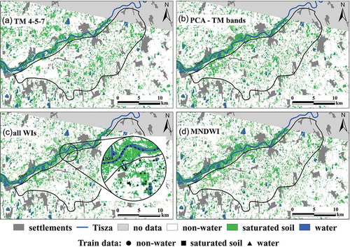
The results of this study show that when a classification was performed on the original bands of the Landsat image, this led to an acceptable outcome with a classification accuracy of 91%. Data show that all six available bands produced the same result (91%) with both RF and SVM; thus, using RF MDA values, we were able to reduce the number of bands involved in the analysis and retain just 4–5–7 (MDAs were 19–32–25, respectively; Fig. 3(a)) so that the MDA of all the others remained below 7%. This band selection process produced a slight improvement in accuracy to 94% when using the SVM classifier (Table 2).

Figure 3. RF classification results using (a) 4–5–7 TM bands; (b) PCA, all TM bands; (c) all WIs; and (d) MNDWI.

3.2 Classification with WIs

We also analysed the identification performance of all calculated WIs in each of our three categories. The results show that MNDWI was by far the best, producing a 98% OA (Table 3; Fig. 3(d)), and was also successful at identifying saturated soils (PA: 93%). However, all the other indices provided only 43–63% accuracy, which is far below the result produced on the basis of the original band approach.

Table 2. Producer’s accuracy of water features and overall accuracy (OA) % of the classifications performed on original Landsat 7 bands using RF and SVM classifiers.

Class	Original bands		4–5–7 bands
	RF	SVM	RF	SVM
Non-water	98	100	100	100
Saturated soil	74	76	78	81
Water	100	97	100	100
OA	91	91	93	94

Table 3. Producer’s accuracy of water features and overall accuracy (OA) % of the classifications performed on WIs derived from Landsat 7 bands using RF and SVM classifiers.

Class	MNDWI		AAVI		NDVI		NDWI Gao		NDWI McFeeters
	RF	SVM	RF	SVM	RF	SVM	RF	SVM	RF	SVM
Non-water	100	100	87	86	99	98	91	92	93	99
Saturated soil	93	91	3	4	9	6	14	5	7	0
Water	100	100	39	56	93	86	83	85	99	99
OA	98	97	43	49	64	63	63	61	67	65
Class	NRVI		RVI		TVI		CTVI		TTVI
	RF	SVM	RF	SVM	RF	SVM	RF	SVM	RF	SVM
Non-water	92	97	98	97	92	97	92	97	92	97
Saturated soil	8	4	9	7	9	7	9	7	9	7
Water	94	86	93	85	94	85	94	85	94	86
OA	65	62	64	63	65	63	65	63	65	63

We repeated the classification step involving all the WIs and showed that with RF it is possible to attain 98% accuracy, although this can also be achieved when just using MNDWI (Table 4; Fig. 3(c)). Next, and in order to avoid overfitting, we also reduced the number of variables based on the MDA values of RF; in this case, accuracy remained at 98% and the most important WIs were the MNDWI (MDA: 57), and the NDWIs (both of McFeeters (1996) and of Gao (1996), with MDA: 17 and 19, respectively; the MDA of all other WIs was <9). The classification accuracy of the saturated soil class was 94% with RF, but this varied between 75 and 78% with SVM, while omitting the Gao NDWI led to a reduction in accuracy of just 1%.

Table 4. Producer’s accuracy of water features and overall accuracy (OA) % of the classifications with all WIs and with a set of WIs (McF: McFeeters).

Class	All WI		Gao + NDWI(McF) + MNDWI		NDWI(McF) + MNDWI
	RF	SVM	RF	SVM	RF	SVM
Non-water	100	100	100	100	100	100
Saturated soil	94	59	94	72	90	75
Water	100	93	100	100	100	100
OA	98	84	98	91	97	92

3.3 PC classification

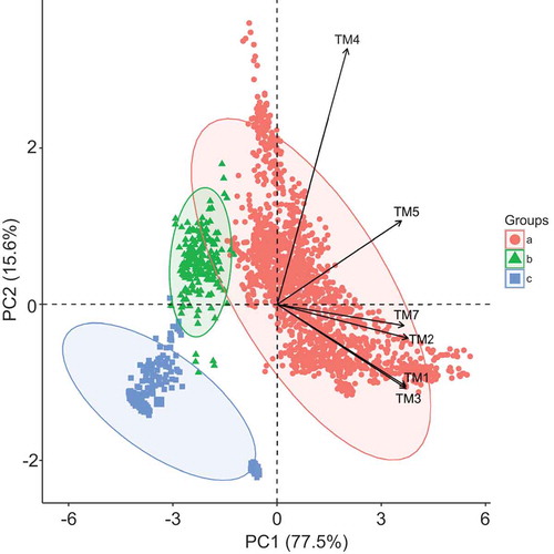
The PCA performed on the original TM bands explained 99.0% of the total variance and justified three PCs; of these, both RMSR and AGFI fit very well (0.01 and 0.99, respectively), while PC1 accounted for 50% of the variance and was correlated with B1–B3, PC2 explained 28% and was correlated with B5 and B7, and PC3 explained 21% and was correlated with B4.

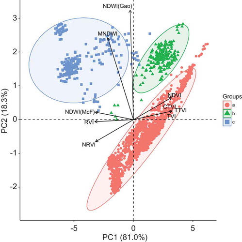
We also performed a PCA including WIs (we excluded the AAVI due to its low communality); this step explained 98.5% of the total variance and resulted in two PCs, justified by the RMSR (0.01) and AGFI (0.99, a very good fit). In this case, PC1 accounted for 72.2% of the variance and was strongly correlated with NRVI, NDVI, RVI, CTVI, TTVI, TVI and NDWI (McFeeters 1996), while PC2 accounted for 26.3% of the variance and was strongly correlated with the remaining two NDWIs, as well as NDWI (Gao 1996) and the MNDWI.

A further bi-plot of this PCA based on TM bands revealed an almost perfect class discrimination with just a small overlap between the non-water and saturated soil classes (Fig. 4). However, both RF (Fig. 3(b)) and SVM resulted in 100% OA (Table 6); the only misclassification in this case was in the use of RF, where one pixel was classified into the saturated soil class instead of as a body of water.

Table 5. Producer’s accuracy of water features and overall accuracy (OA) %of the classifications performed on PCs derived from original Landsat 7 bands (TM bands) and WIs, using RF and SVM classifiers.

Class	PCA (WIs)		PCA (TM bands)
	RF	SVM	RF	SVM
Non-water	100	100	100	100
Saturated soil	99	99	100	100
Water	98	100	99	100
OA	99	100	100	100

Table 6. Distribution of water-related categories by land-cover classes of CLC 2000 (minimum and maximum values).

CLC code	CLC type	Proportion of CLC type (%)	Non-water (%)	Saturated soil (%)	Water (%)	NDVI mean ± SD
112	Discontinuous urban fabric	4.30	3.83–4.20	0.09–0.45	0.01–0.02	–0.08 ± 0.10
211	Non-irrigated arable land	68.66	57.67–59.66	8.33–10.17	0.68–0.88	–0.05 ± 0.18
222	Fruit trees and berry plantations	1.46	1.26–1.43	0.03–0.2	0	0.11 ± 0.10
231	Pastures (grassland)	15.38	11.50–12.02	3.12–3.66	0.22–0.25	0.13 ± 0.15
242	Complex cultivation	2.76	2.41–2.48	0.25–0.32	0.02–0.03	–0.01 ± 0.13
243	Agriculture with natural vegetation	3.12	2.20–2.22	0.78–0.80	0.11–0.12	0.02 ± 0.15
311	Broad-leaved forest	1.62	1.03–1.20	0.39–0.56	0.03–0.04	0.14 ± 0.15
324	Transitional woodland shrub	0.50	0.34–0.35	0.12–0.16	0.01	0.16 ± 0.13
0.13	Inland marshes	1.75	0.97–1.03	0.67–0.73	0.06–0.07	0.01 ± 0.13
512	Water bodies	0.44	0.02–0.03	0.07–0.08	0.33–0.34	–0.26 ± 0.14

Figure 4. Bi-plot diagram of the PCs derived from TM bands (categories are grouped by colours: (a) non-water; (b) saturated soil; (c) water; 95% ellipses).

The bi-plot diagram of WIs, PC1 and PC2 revealed good discrimination between the categories of water-related features (Fig. 5). In this case, classification accuracy was 99% for RF and 100% for SVM; there were four pixel misclassifications using RF and just one for SVM (Table 5).

Figure 5. Bi-plot diagram of the PCs derived from WIs (categories are grouped by colours: (a) non-water; (b) saturated soil; (c) water; 95% ellipses).

3.4 Uncertainty of CLC class classifications

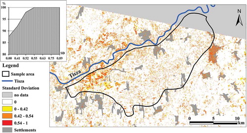
We calculated uncertainty from the following outcomes (input data and classifier) based on their relative performance (>98% OA): (a) PCs derived from TM bands with RF; (b) PCs derived from TM bands with SVM; (c) TM bands with RF; (d) WIs with RF; (e) Gao + NDWI + MNDWI with RF; (f) MNDWI with RF; and (g) PCs derived from WIs with SVM. The average SD was the largest in the case of linear artificial landscape elements summarized by CLC categories (i.e. roads and railways, Table 6), while the second largest value belonged to the water body class. This result indicates that, although these methods produced a good performance, there were relevant differences in terms of spatial projection.

The distribution of the calculated SD is shown in Figure 6. According to the six most accurate classification methods, more than half of the interpreted area is classified with maximal certainty (SD = 0). Larger SDs can be detected in the western part of the sample area, mostly covered by high clay-content sediments where persistent shallow water cover (or inland inundation) can occur.

Figure 6. Map of standard deviation (SD) calculated from the six most accurate classifications including the cumulative histogram of the SD values.

According to the proportional distribution of water-related categories based on classification by CLC class, we found that the category of saturated soils belongs to non-irrigated arable lands and pastures (Table 7). The NDVI values had large variance, indicating varied distribution and proportion of water features. However, while in the case of arable lands or pastures, negative values can refer to the presence of water, the “discontinuous urban fabric” class had artificial causes.

Table 7. Classification uncertainty of the best six classified maps (PCs derived from TM bands with RF; TM bands with RF; 4–5–7 TM bands with SVM; PCs derived from WIs with SVM; WIs with RF; MNDWI with RF) considering the standard deviation (SD) of the categories by CLC class.

CLC code	CLC class	Average SD by CLC class
512	Water body	0.252
324	Transitional woodland shrub	0.210
222	Fruit trees and berry plantations	0.145
311	Broad-leaved forest	0.138
112	Discontinuous urban fabric	0.133
231	Pastures (grassland)	0.126
243	Land principally occupied by agriculture, with significant areas of natural vegetation	0.120
211	Non-irrigated arable land	0.117
242	Complex cultivation	0.116
411	Inland marsh	0.079

3.5 Confirmation of the extraction of water-related features

The classification performed on the 2006 satellite image resulted in good results with an accuracy of 96–98% OA. In this case, PCs of PCA (either with TM bands or with WIs) did not perform better than the original variables and resulted in a slightly (1%) weaker accuracy (Table 8). The PCs were the most efficient to identify dry areas and water bodies but had misclassifications for saturated soils.

Table 8. Classification accuracies of the Landsat 5 image of 19 June 2006 using different input data (WIs: water indices; TM bands; and PCs of PCA solutions) and classification algorithms. RF: random forest; SVM: support vector machine.

Category	MNDWI (RF)	All WI (RF)	Gao + NDWI + MNDWI (RF)	PCA WIs (RF)	PCA WIs (SVM)	PCA TM bands (RF)	PCA TM bands (SVM)
Dry area	97	99	100	99	100	100	100
Saturated soil	96	96	96	93	91	96	95
Water body	98	100	99	99	100	99	100
OA	97	98	98	97	97	98	98

4 Discussion

A classification based on the original bands of a Landsat 7 image, as well as a WI-based classification, and ordinations (PCA) of TM bands and WIs represent four distinct approaches to identify water bodies, saturated soils and non-water areas. Traditional methods, using original bands, have usually been used for mapping land cover (Keuchel et al. 2003, Cingolani et al. 2004, Churches et al. 2014), to monitor changes in the surface based on multi-temporal images (Fichera et al. 2012), and to determine different urban surfaces, e.g. roofing materials (Szabó et al. 2014). However, OA values obtained using these methods were rarely above 90%. In contrast, other studies (Gao 1996, de Alwis et al. 2007) calculated spectral indices, and, with optimal thresholds, the accuracy in these cases, e.g. for water detection (McFeeters 1996), reached more than 99%. This kind of PCA-based classification has been widely applied, especially for change analysis; this method can reduce the dimensions of multi-temporal datasets and, using PCs, the areas most subject to change can be detected. Many authors have calculated PCs from original spectral bands (e.g. Munyati 2004, Khan et al. 2005, Forzieri et al. 2011, Kit et al. 2012), but these can also be determined from various sets of variables (Byrne et al. 1980, Richards 1984), or from spectral index time series (Hirosawa et al. 1996, Mills et al. 2013, Dronova et al. 2015). The accuracy demonstrated with PCA-based methodology varies in the relevant literature, and depends on the feature classes involved (Table 9).

Table 9. Accuracy of image analysis techniques by the data types involved in previous studies.

Author	Study area	Image	Accuracy	Note
Original bands
Keuchel et al. (2003)	Tenerife, Spain	Landsat	90%	Land-cover detection
Cingolani et al. (2004)	Argentina	Landsat	78%	Vegetation mapping
Atkinson (2004)	–	Simulated images	89–93%
Fichera et al. (2012)	Avellino, Italy	Landsat	86–95%	Land-cover change
Churches et al. (2014)	Haiti	Landsat	78%	Forest detection
Szabó et al. (2014)	Debrecen, Hungary	Airborne hyperspectral data	~85%	Asbestos roof identification
Spectral indices
de Alwis et al. (2007)	Town Brook, USA	Landsat	78–79%	Land-cover detection
Xu (2006)	Xiamen City; Luoyuan Bay; Min River, China	Landsat	99.85%	Water detection
Fisher and Danaher (2013)	New South Wales, Australia	SPOT	98%	LDAWI for water detection
PCA-based
Byrne et al. (1980)	Batemans Bay, New South Wales, Australia	Landsat		Land-cover change detection
Richards (1984)	New South Wales, Australia	Landsat		Change detection (bush fire)
Hirosawa et al. (1996)	Arizona, USA	AVHRR		Vegetation mapping
Munyati (2004)	Kaufe Flats, Zambia	Landsat
Khan et al. (2005)	Indus Basin, Pakistan	IRS LISS-II		Salt-affected soils detection
Koutsias et al. (2009)	Island of Samos, Greece	Landsat	Separability value was used: 1.89	Burnt land mapping, change detection
Forzieri et al. (2011)	Avisio River, Italy	SPOT-5	69.29%, Kappa 0.78	Land-cover extraction
Kit et al. (2012)	Hyderabad, India	QuickBird	Identification probability: 83.33%	Slum detection
Mills et al. (2013)	Southern Rockies–Colorado Plateau, USA	MODIS		Change detection
Dronova et al. (2015)	Poyang Lake, China	Beijing-1; ASAR	94.7% OA, Kappa 0.938	Land-cover mapping

Generally speaking, all the methods applied in this paper performed well, but usually exhibited classification errors when addressing the saturated soil class. This transitional category experienced most problems because we often identified a type of vegetation for this category and not the bare moist topsoil itself due to land cover. The situation was similar to that for the dry, non-water-related soil class, but was more obvious; if the soil is dry, the vegetation also reflects this. This means that a higher proportion of saturated soil misclassifications occurred with dry surfaces rather than with water bodies. This is noteworthy because, although the discrimination of water bodies seemed straightforward, they are not pure surfaces; thus, uncertainty analysis revealed that these areas, as well as transitional woodland shrub classes, had the largest variance through the six classes, leading to inaccurate results (Table 6). Permanent water bodies are also often covered with aquatic vegetation and surface water submerges grasslands and pastures, which can also add bias to the classification; shoreline areas were also misclassified in some cases, a result similar to that reported by Zlinszky et al. (2015).

The dominant land-cover type within the area discussed in this study was arable land, including all water-related categories. Mostly, however, this land-use type was considered as non-water (83–84%), although a smaller proportion was classified as saturated soil (14–15%) and as a water body in cases where the ratio was less than 1%, which is related to the high (68%) proportion of arable lands (Table 7). Considering the intensive rainfall and groundwater persistence during this period of the year, both dry areas and wet conditions can occur; this means that sand dunes are already dry while the valleys between them are still wet. Furthermore, arable land is covered with different types of plants in different phenophases, which biases the spectral features of the area. The results of this study nevertheless corroborate the idea that, in spite of various influencing factors, we are able to discriminate different water content classes. Pastures were mostly classified within the non-water category (74–75%) and as saturated soil (20–21%). Therefore, considering that NDVI values are usually negative in the case of water bodies and arable lands, and pastures had large variance for NDVI (Table 7), it is likely that these areas were inundated or in saturated states.

Compared to the satellite-based classification performed using an original WI-based band approach, use of MNDWI yielded better accuracy for both water bodies and wetlands. However, although PCA, especially with MNF transformation (Frassy et al. 2013), is often used successfully for hyperspectral images, i.e. a large number of bands (Rodarmel and Shan 2002), the best performance in this study was achieved via the use of PCs with just a few bands: the results show that both the PCA performed on the original bands and the one performed on WIs provided the most accurate results. Furthermore, misclassification errors per class were almost zero, between just one and four pixels were classified into another class in each case. RF usually provided slightly better results than SVM; however, when the PCs were introduced (which provided the best outcomes), SVM was the better classifier.

Taking into account all the input data used during this study, the most favourable option was to use the PCs of the original band ordination. Although WIs have usually performed better in other studies, we only achieved good results at a convincing level of accuracy in this case with MNDWI, as all other WIs had only 60–70% OA values. Although it is possible that WIs might provide better results via the addition of more dimensions, including two or more variables/bands (Afifi et al. 2012), in this case they did not augment any combinations either on their own, together, or as PCs in the creation of more accurate maps. In a similar work, Fisher and Danaher (2013) also applied the multivariate linear discriminant analysis (LDA) method using original bands and their linear combinations, and then compared their results with the McFeeters (1996) and Xu (2006) NDWIs. These authors all found that their multivariate approach performed with a higher degree of accuracy in identifying water bodies, as in this study. However, PCA without a target variable provided an errorless outcome in our case using just original bands. Our final conclusion is therefore that PCA increased the accuracy of class identifications with different water contents, while of the WIs, just the MNDWI was efficient.

Our confirmation analysis shows that a final classification outcome can be exact and report the right information, whether or not the extraction of water-related features is repeatable. This depends, however, on designating the right training areas using satellite image and auxiliary data sources, including the thematic map of surface water patches and aerial images. It is also important to ensure that training areas are carefully delineated, following the traces of current or former water cover, and that all collected information should correspond with the satellite image. In other words, only patches are allowed that can be found on both data sources. Our second analysis using the 2006 Landsat 5 satellite image required a new training dataset, as water-related features change temporally and depend on the level of soil saturation, precipitation and the combination of the two. In other words, it is important to know the saturation level due to melting snow after precipitation has fallen on the area in the spring. Our new analysis resulted in similar results to the previous statements except that PCA did not ensure better thematic accuracy: dry areas and water bodies were identified almost perfectly, but, as we pointed out previously, saturated soil, the transitional category, had misclassification issues. This means only 1% less OA and issues can originate from two sources: land cover of dry and saturated areas has similar reflectance profiles and their interspersion is natural, and/or training areas contained some pixel(s) belonging to the other category (Ozesmi and Bauer 2002).

Although satellite images enable a wide range of information extraction possibilities, they are nevertheless archive data, and thus it is always a challenge to collect the right information to validate the results of their processing. Our approach for data collection using direct (maps of water authorities) and indirect (with auxiliary data, i.e. searching the clues to saturated soils using aerial images) presents one possible solution. The method also has its limitations, but the final results are accurate, with a minimum OA of 97% and PA of 91%. Success depends on the given situation in a specific year and the date when the image was captured: when the amount of precipitation is large, and the image is captured close to the maximal extent of patches of pluvial flood, the predictable accuracy is good. However, when there is a time lag between the maximal extent and the date of the available image, or the amount of precipitation is not enough to fill all the possible sinks, the accuracy can be lower. This was the case with the image of 2006, when the classification performance was 91–96% (regarding the PA), which was lower but still acceptable compared to the image of 2000, where we obtained 98–99% PA.

Given the local future climate change scenarios for the Carpathian Basin, increasing drought sensitivity and extremes of weather have to be considered (Mika 2013, Ladányi et al. 2015). In view of the changing distribution of precipitation in both time and space, according to earlier predictions (Bartholy et al. 2009), periods of drought may last longer and surface water may be formed, both phenomena that threaten agricultural production. Therefore, research investigating water resources will also play a significant role in the future. The approach presented here can contribute to mapping those areas that are relevant for water management, where agricultural production will be threatened by the risk of drought, and where, as a consequence, the installation of watering systems will be needed, or crop type selection should be considered in line with the severity of decreasing water resources. Although this study has only dealt with the mapping phase itself, this methodology can also be used to reveal spatial and temporal trends.

5 Conclusions

Four approaches were tested in this study: (a) original bands; (b) WIs; (c) PCA conducted on original bands; and (d) PCA conducted on WIs. The performance of original bands was acceptable, with an overall accuracy of 93%. However, the use of WIs did not help to improve the outcomes, as their performance was between 60 and 70%, with the exception of MNDWI, which was very effective, with an overall accuracy of 98%. Combining the WIs did not bring any increase; in fact, the accuracy decreased to 96%. However, PCA, conducted both on the original bands and on WIs, had the best performance, with a 99–100% overall accuracy. SVM performed on the original bands provided slightly better results than RF. Although more variables can generally improve the accuracy of the classifications, only one WI (MNDWI) had a particularly good performance; in this case, the other variables reduced it and, therefore, PCA performed on the WIs was not as successful as was the case with original bands. Calculating standard deviation from different classification results can reveal the uncertainty of the classifications. Although there are limitations of the satellite images in mapping the water and water-related features, this study confirmed their applicability.

Disclosure statement

No potential conflict of interest was reported by the authors.

Additional information

Funding

The research of Boglárka Balázs was supported by the European Union and the State of Hungary, co-financed by the European Social Fund in the framework of the TÁMOP 4.2.4.A/2-11-1-2012-0001 “National Excellence Program”. The publication was supported by the SROP-4.2.2.B-15/1/KONV-2015-0001 project, the National Research, Development and Innovation Office (NKFIH; 108755), and by the University of Debrecen (RH/751/2015). The project is supported by the European Union, co-financed by the European Social Fund.

References

- Afifi, A., May, S., and Clark, V., 2012. Practical multivariate analysis. Boca Raton: CRC Press.
- Alsdorf, D.E., et al., 2000. Interferometric radar measurements of water level changes on the Amazon flood plain. Nature, 404, 174–177. doi:10.1038/35004560
- Aly, A.A., et al., 2016. Vegetation cover change detection and assessment in arid environment using multi-temporal remote sensing images and ecosystem management approach. Solid Earth, 7, 713–725. doi:10.5194/se-7-713-2016
- Amari, S. and Wu, S., 1999. Improving support vector machine classifiers by modifying kernel functions. Neural Networks, 12, 783–789. doi:10.1016/S0893-6080(99)00032-5
- Ashburn, P., 1979. The vegetative index number and crop identification. In: Proceedings of the technical session, Houston, TX, Vols. 1–2. NASA. Johnson Space Center Proc. of Tech., 843–855.
- Atkinson, P.M., 2004. Spatially weighted supervised classification for remote sensing. International Journal of Applied Earth Observation and Geoinformation, 5, 277–291. doi:10.1016/j.jag.2004.07.006
- Baret, F. and Guyot, G., 1991. Potentials and limits of vegetation indices for LAI and APAR assessment. Remote Sensing of Environment, 35, 161–173. doi:10.1016/0034-4257(91)90009-U
- Barnett, T., et al., 2004. The effects of climate change on water resources in the west: introduction and overview. Climatic Change, 62, 1–11. doi:10.1023/B:CLIM.0000013695.21726.b8
- Bartholy, J., et al., 2009. Analysis of regional climate change modelling experiments for the Carpathian Basin. International Journal of Global Warming, 1, 238–252. doi:10.1504/IJGW.2009.027092
- Basto, M. and Pereira, J.M., 2012. An SPSS R-menu for ordinal factor analysis. Journal of Statistical Software, 46 (4), 1–29. doi:10.18637/jss.v046.i04
- Bernaards, C.A. and Jennrich, R.I., 2005. Gradient projection algorithms and software for arbitrary rotation criteria in factor analysis. Educational and Psychological Measurement, 65, 676–696. doi:10.1177/0013164404272507
- Breiman, L., 2001. Random forests. Machine Learning, 45, 5–32. doi:10.1023/A:1010933404324
- Burai, P., et al., 2015. Classification of herbaceous vegetation using airborne hyperspectral imagery. Remote Sensing, 7, 2046–2066. doi:10.3390/rs70202046
- Byrne, G.F., Crapper, P.F., and Mayo, K.K., 1980. Monitoring land-cover change by principal component analysis of multitemporal Landsat data. Remote Sensing of Environment, 10, 175–184. doi:10.1016/0034-4257(80)90021-8
- Chen, X.-L., et al., 2006. Remote sensing image-based analysis of the relationship between urban heat island and land use/cover changes. Remote Sensing of Environment, 104, 133–146. doi:10.1016/j.rse.2005.11.016
- Churches, C.E., et al., 2014. Evaluation of forest cover estimates for Haiti using supervised classification of Landsat data. International Journal of Applied Earth Observation and Geoinformation, 30, 203–216. doi:10.1016/j.jag.2014.01.020
- Cingolani, A.M., et al., 2004. Mapping vegetation in a heterogeneous mountain rangeland using Landsat data: an alternative method to define and classify land-cover units. Remote Sensing of Environment, 92, 84–97. doi:10.1016/j.rse.2004.05.008
- Clark Labs, 2012. IDRISI Selva. Worcester: Clark University.
- CLC 2000, Corine Land Cover Programme, EEA. http://www.eea.europa.eu/data-and-maps/data/corine-land-cover-2000-clc2000-seamless-vector-database [Accessed September 2016].
- Congalton, R.G., 1991. A review of assessing the accuracy of classifications of remotely sensed data. Remote Sensing of Environment, 37, 35–46. doi:10.1016/0034-4257(91)90048-B
- Davis, J.C., 1986. Statistics and data analysis in geology. 2nd ed. New York: Wiley.
- de Alwis, D.A., et al., 2007. Unsupervised classification of saturated areas using a time series of remotely sensed images. Hydrology and Earth System Sciences, 11, 1609–1620. doi:10.5194/hess-11-1609-2007
- Deering, D.W., et al., 1975. Measuring “forage production” of grazing units from Landsat MSS data. In: Proceedings of the 10th International Symposium on Remote Sensing of Environment, Vol. 2, Ann Arbor: ERIM, 1169–1178.
- Demetriades-Shah, T.H., Steven, M.D., and Clark, J.A., 1990. High resolution derivative spectra in remote sensing. Remote Sensing of Environment, 33, 55–64. doi:10.1016/0034-4257(90)90055-Q
- Deng, J.S., et al., 2008. PCA-based land-use change detection and analysis using multitemporal and multisensor satellite data. International Journal of Remote Sensing, 29, 4823–4838. doi:10.1080/01431160801950162
- Di Baldassarre, G., Schumann, G., and Bates, P.D., 2009. A technique for the calibration of hydraulic models using uncertain satellite observations of flood extent. Journal of Hydrology, 367 (3–4), 276–282. doi:10.1016/j.jhydrol.2009.01.020
- Dronova, I., et al., 2015. Mapping dynamic cover types in a large seasonally flooded wetland using extended principal component analysis and object-based classification. Remote Sensing of Environment, 158, 193–206. doi:10.1016/j.rse.2014.10.027
- Eklundh, L. and Singh, A., 1993. A comparative analysis of standardised and unstandardised principal components analysis in remote sensing. International Journal of Remote Sensing, 14, 1359–1370. doi:10.1080/01431169308953962
- Estoque, R.C. and Murayama, Y., 2015. Classification and change detection of built-up lands from Landsat-7 ETM+ and Landsat-8 OLI/TIRS imageries: A comparative assessment of various spectral indices. Ecological Indicators, 56, 205–217. doi:10.1016/j.ecolind.2015.03.037
- Fichera, C.R., Modica, G., and Pollino, M., 2012. Land cover classification and change-detection analysis using multi-temporal remote sensed imagery and landscape metrics. European Journal of Remote Sensing, 45, 1–18. doi:10.5721/EuJRS20124501
- Fisher, A. and Danaher, T., 2013. A water index for SPOT5 HRG satellite imagery, New South Wales, Australia, determined by linear discriminant analysis. Remote Sensing, 5 (11), 5907–5925. doi:10.3390/rs5115907
- Forzieri, G., et al., 2011. Satellite multispectral data for improved floodplain roughness modelling. Journal of Hydrology, 407, 41–57. doi:10.1016/j.jhydrol.2011.07.009
- Frassy, F., et al., 2013. Minimum noise fraction transform for improving the classification of airborne hyperspectral data: two case studies. In: 5th Workshop on hyperstectral image and signal processing: evolution in remote sensing, Gainesville, FL: IEEE, 1–4. doi:10.1109/WHISPERS.2013.8080626.
- Gabriel, K.R., 1971. The bi-plot graphic display of matrices with application to principal component analysis. Biometrika, 58, 453–467. doi:10.1093/biomet/58.3.453
- Gao, B.-C., 1996. NDWI—a normalized difference water index for remote sensing of vegetation liquid water from space. Remote Sensing of Environment, 58, 257–266. doi:10.1016/S0034-4257(96)00067-3
- Gu, Y., et al., 2008. Evaluation of MODIS NDVI and NDWI for vegetation drought monitoring using Oklahoma Mesonet soil moisture data. Geophysical Research Letters, 35, L22401. doi: 10.1029/2008GL035772
- Hegedüs, P., et al., 2015. Analysis of spatial variability of near-surface soil moisture to increase rainfall-runoff modelling accuracy in SW Hungary. Open Geosciences, 7, 126–139. doi:10.1515/geo-2015-0017
- Hirosawa, Y., Stuart, E.M., and Kliman, D.H., 1996. Application of standardized principal component analysis to land-cover characterization using multitemporal AVHRR data. Remote Sensing of Environment, 58, 267–281. doi:10.1016/S0034-4257(96)00068-5
- Ho, T.K., 1995. Random decision forests. In: Proceedings of the 3rd international conference on document analysis and recognition, Montreal, QC, 14–16 August 1995. IEEE Computer Society, 278–282.
- Jaccard, J. and Wan, C.K., 1996. LISREL approaches to interaction effects in multiple regression. London: Quantitative Applications in the Social Sciences, SAGE Publications.
- Jin, S., Li, D., and Wang, J., 2005. A comparison of support vector machine with maximum likelihood classification algorithms on texture features. In: Proceedings. IEEE international geoscience and remote sensing symposium, IGARSS ‘05, Vol. 5, 3717–3720. doi:10.1109/IGARSS.2005.1526659
- Jolliffe, I.T., 2002. Principal component analysis. 2nd ed. New York: Springer.
- Jöreskug, K. and Sörbom, D., 1996. LISREL 8: user’s reference guide. Lincolnwood: Scientific Software International.
- Kassambara, A. and Mundt, F., 2017. Factoextra: extract and visualize the results of multivariate data analyses. R package version 1.0.4. https://CRAN.R-project.org/package=factoextra [Accessed September 2017].
- Keuchel, J., et al., 2003. Automatic land cover analysis for Tenerife by supervised classification using remotely sensed data. Remote Sensing of Environment, 86, 530–541. doi:10.1016/S0034-4257(03)00130-5
- Khan, N.M., et al., 2005. Assessment of hydrosaline land degradation by using a simple approach of remote sensing indicators. Agricultural Water Management, 77, 96–109. doi:10.1016/j.agwat.2004.09.038
- Kit, O., Lüdeke, M., and Reckien, D., 2012. Texture-based identification of urban slums in Hyderabad, India using remote sensing data. Applied Geography, 32, 660–667. doi:10.1016/j.apgeog.2011.07.016
- Ko, B.C., Kim, H.H., and Nam, J.Y., 2015. Classification of potential water bodies using landsat 8 OLI and a combination of two boosted random forest classifiers. Sensors, 15, 13763–13777. doi: 10.3390/s150613763
- Kohler, U. and Luniak, M., 2005. Data inspection using bi-plots. The Stata Journal, 5, 208–223.
- Koutsias, N., Mallinis, G., and Karteris, M., 2009. A forward/backward principal component analysis of Landsat-7 ETM+ data to enhance the spectral signal of burnt surfaces. ISPRS Journal of Photogrammetry and Remote Sensing, 64, 37–46. doi:10.1016/j.isprsjprs.2008.06.004
- Kumar, D., 2015. Remote sensing based vegetation indices analysis to improve water resources management in urban environment. Aquatic Procedia, 4, 1374–1980. doi:10.1016/j.aqpro.2015.02.178
- Kuti, L., Kerék, B., and Vatai, J., 2006. Problem and prognosis of excess water inundation based on agrogeological factors. Carpathian Journal of Earth and Environmental Sciences, 1, 5–18.
- Lê, S., Josse, J., and Husson, F., 2008. FactoMineR: an R package for multivariate analysis. Journal of Statistical Software, 25 (1), 1–18. doi:10.18637/jss.v025.i01
- Ladányi, Z., et al., 2015. Multi-indicator sensitivity analysis of climate change effects on landscapes in the Kiskunság National Park, Hungary. Ecological Indicators, 58, 8–20. doi:10.1016/j.ecolind.2015.05.024
- Li, X., et al., 2013. Comparative study of water-body information extraction methods based on electronic sensing image. Lecture Notes in Electrical Engineering, 178, 331–336. doi:10.1007/978-3-642-31528-2_52
- Liu, J., Pattey, E., and Jégo, G., 2012. Assessment of vegetation indices for regional crop green LAI estimation from Landsat images over multiple growing seasons. Remote Sensing of Environment, 123, 347–358. doi:10.1016/j.rse.2012.04.002
- Louppe, G., et al., 2013. Understanding variable importances in forests of randomized trees. In: Advances in neural information processing systems. NIPS proceedings, 431–439. Neural Information Processing Systems Conference, Lake Tahoe. Neural Information Processing Systems Foundation, Inc.
- Lu, D., et al., 2014. Methods to extract impervious surface areas from satellite images. International Journal of Digital Earth, 7, 93–112. doi:10.1080/17538947.2013.866173
- Lu, D. and Weng, Q., 2007. A survey of image classification methods and techniques for improving classification performance. International Journal of Remote Sensing, 28, 823–870. doi:10.1080/01431160600746456
- Marshall, M. and Thenkabail, P., 2015. Advantage of hyperspectral EO-1 Hyperion over multispectral IKONOS, GeoEye-1, WorldView-2, Landsat ETM+, and MODIS vegetation indices in crop biomass estimation. ISPRS Journal of Photogrammetry and Remote Sensing, 108, 205–218. doi:10.1016/j.isprsjprs.2015.08.001
- McFeeters, S.K., 1996. The use of the Normalized Difference Water Index (NDWI) in the delineation of open water features. International Journal of Remote Sensing, 17, 1425–1432. doi:10.1080/01431169608948714
- Meglen, R.R., 1992. Examining large databases: a chemometric approach using principal component analysis. Marine Chemistry, 39, 217–237. doi:10.1016/0304-4203(92)90103-H
- Melesse, A.M. and Shih, S.F., 2002. Spatially distributed storm runoff depth estimation using Landsat images and GIS. Computers and Electronics in Agriculture, 37, 173–183. doi:10.1016/S0168-1699(02)00111-4
- Mika, J., 2013. Meteorological extremes and their changes: phenomenology and empirical aproaches. Climatic Change, 121, 15–26. doi:10.1007/s10584-013-0914
- Mills, R.T., et al., 2013. Identification and visualization of dominant patterns and anomalies in remotely sensed vegetation phenology using a parallel tool for principal components analysis. Procedia Computer Science, 18, 2396–2405. doi:10.1016/j.procs.2013.05.411
- Mukherjee, S., et al., 2006. Learning theory: stability is sufficient for generalization and necessary and sufficient for consistency of empirical risk minimization. Advances in Computational Mathematics, 25, 161–193. doi:10.1007/s10444-004-7634-z
- Munyati, C., 2004. Use of principal component analysis (PCA) of remote sensing images in wetland change detection on the Kafue Flats, Zambia. Geocarto International, 19, 11–22. doi:10.1080/10106040408542313
- Narasimhan, B. and Srinivasan, R., 2005. Development and evaluation of Soil Moisture Deficit Index (SMDI) and Evapotranspiration Deficit Index (ETDI) for agricultural drought monitoring. Agricultural and Forest Meteorology, 133, 69–88. doi:10.1016/j.agrformet.2005.07.012
- Nyarko, B.K., et al., 2015. Floodplain wetland mapping in the White Volta River Basin of Ghana. GIScience & Remote Sensing, 52, 374–395. doi:10.1080/15481603.2015.1026555
- Otukei, J.R. and Blaschke, T., 2010. Land cover change assessment using decision trees, support vector machines and maximum likelihood classification algorithms. International Journal of Applied Earth Observation and Geoinformation, 12 (S1), S27–S31. doi:10.1016/j.jag.2009.11.002
- Ozesmi, S. and Bauer, M.E., 2002. Satellite remote sensing of wetlands. Wetlands Ecology and Management, 10, 381–402. doi:10.1023/A:1020908432489
- Pal, M., 2005. Random forest classifier for remote sensing classification. International Journal of Remote Sensing, 26, 217–222. doi:10.1080/01431160412331269698
- Pásztor, L., et al., 2015. Spatial risk assessment of hydrological extremities: inland excess water hazard, Szabolcs-Szatmár-Bereg County, Hungary. Journal of Maps, 11, 636–644. doi:10.1080/17445647.2014.954647
- Pásztor, L., et al., 2016. Integrated spatial assessment of wind erosion risk in Hungary. Natural Hazards and Earth System Sciences, 16, 2421–2432. doi:10.5194/nhess-16-2421-2016
- Perry Jr., C. and Lautenschlager, L.F., 1984. Functional equivalence of spectral vegetation indices. Remote Sensing of Environment, 14, 169–182. doi:10.1016/0034-4257(84)90013-0
- R Core Team, 2016. R: a language and environment for statistical computing. Vienna: R Foundation for Statistical Computing. https://www.R-project.org/ [Accessed 10 May 2015].
- Revelle, W., 2015. psych: procedures for personality and psychological research. Evanston: Northwestern University. http://CRAN.R-project.org/package=psych [Accessed September 2017].
- Richards, J.A., 1984. Thematic mapping from multitemporal image data using the principal components transformation. Remote Sensing of Environment, 16, 35–46. doi:10.1016/0034-4257(84)90025-7
- Richardson, A.J. and Wiegand, C.L., 1977. Distinguishing vegetation from soil background information. Photogramnetric Engineering and Remote Sensing, 43, 1541–1552.
- Rodarmel, C. and Shan, J., 2002. Principal component analysis for hyperspectral image classification. Surveying and Land Information Science, 62, 115–122.
- Rouse, Jr., J.W., et al., 1974. Monitoring the vernal advancement and retrogradation (green wave effect) of natural vegetation. In: NASA/GSFC type III final report, Greenbelt, MD, 371. Texas A&M University, Remote Sensing Center.
- Sawaya, K.E., et al., 2003. Extending satellite remote sensing to local scales: land and water resource monitoring using high-resolution imagery. Remote Sensing of Environment, 88, 144–156. doi:10.1016/j.rse.2003.04.006
- Schölkopf, B., et al., 1997. Comparing support vector machines with Gaussian kernels to radial basis function classifiers. IEEE Transactions on Signal Processing, 45, 2758–2765. doi:10.1109/78.650102
- Schowengerdt, R.A., 2007. Remote sensing. San Diego: Academic Press – Elsevier.
- Singh, A., 1989. Digital change detection techniques using remotely-sensed data. International Journal of Remote Sensing, 10 (6), 989–1003. doi:10.1080/01431168908903939
- Sonka, M., Hlavac, V., and Boyle, R., 2014. Image processing, analysis, and machine vision. 4h ed. Stamford: Cengage Learning.
- Srivastava, P.K., et al., 2012. Selection of classification techniques for land use/land cover change investigation. Advances in Space Research, 50, 1250–1265. doi:10.1016/j.asr.2012.06.032
- Szabó, S., et al., 2014. Testing algorithms for the identification of asbestos roofing based on hyperspectral data. Environmental Engineering and Management Journal, 143, 2875–2880.
- Szabó, S., Gácsi, Z., and Balázs, B., 2016. Specific features of NDVI, NDWI and MNDWI as reflected in land cover categories. Acta Geographica Debrecina Landscape and Environment, 10 (3–4), 194–202. doi:10.21120/LE/10/3-4/13
- Thiam, A.K., 1997. Geographic information systems and remote sensing methods for assessing and monitoring land degradation in the Sahel: the case of Southern Mauritania. Dissertation. Clark University, Worcester Massachusetts.
- van den Berg, R.A., et al., 2006. Centering, scaling, and transformations: improving the biological information content of metabolomics data. BMC Genomics, 7, 142. doi:10.1186/1471-2164-7-142
- van Leeuwen, B., et al., 2012. Identification of inland excess water floodings using an artificial neural network. Carpathian Journal of Earth and Environmental Sciences, 7, 173–180.
- Vapnik, V., 1995. The nature of statistical learning theory. New York: Springer-Verlag.
- Vörösmarty, C.J., et al., 2000. Global water resources: vulnerability from climate change and population growth. Science, 289, 284–288. doi:10.1126/science.289.5477.284
- Wallace, J., Behn, G., and Furby, S., 2009. Vegetation condition assessment and monitoring from sequences of satellite imagery. Ecological Management and Restoration, 7, S31–S36. doi:10.1111/j.1442-8903.2006.00289.x
- Water Quality Report, 2000. Chronology of the flood of spring of 2000. Vol. 7. Szolnok: Environmental Agency of the Middle-Tisza Region, 1–8 (in Hungarian).
- Weng, Q., 2012. Remote sensing of impervious surfaces in the urban areas: requirements, methods, and trends. Remote Sensing of Environment, 117, 34–49. doi:10.1016/j.rse.2011.02.030
- Williams, G.J., 2011. Data mining with Rattle and R: the art of excavating data for knowledge discovery, use R! New York: Springer.
- Wright, C. and Gallant, A., 2007. Improved wetland remote sensing in Yellowstone National Park using classification trees to combine TM imagery and ancillary environmental data. Remote Sensing of Environment, 107, 582–605. doi:10.1016/j.rse.2006.10.019
- Xu, H., 2005. A study on information extraction of water body with the Modified Normalized Difference Water Index (MNDWI). Journal of Remote Sensing, 9, 589–595.
- Xu, H., 2006. Modification of normalised difference water index (NDWI) to enhance open water features in remotely sensed imagery. International Journal of Remote Sensing, 27, 3025–3033. doi:10.1080/01431160600589179
- Zlinszky, A., et al., 2015. Mapping Natura 2000 habitat conservation status in a pannonic salt steppe with airborne laser scanning. Remote Sensing, 7, 2991–3019. doi:10.3390/rs70302991