An improved nonstationary model for flood frequency analysis and its implication for the Three Gorges Dam, China

ABSTRACT

This study proposes an improved nonstationary model for flood frequency analysis by investigating the relationship between flood peak and flood volume, using the Three Gorges Dam (TGD), China, for verification. First, the generalized additive model for location, scale and shape (GAMLSS) is used as the prior distribution. Then, under Bayesian theory, the prior distribution is updated using the conditional distribution, which is derived from the copula function. The results show that the improvement of the proposed model is significant compared with the GAMLSS-based prior distribution. Meanwhile, selection of a suitable prior distribution has a significant effect on the results of the improvement. For applications to the TGD, the nonstationary model can obviously increase the engineering management benefits and reduce the perceived risks of large floods. This study provides guidance for the dynamic management of hydraulic engineering under nonstationary conditions.

KEYWORDS:

• nonstationary model
• flood frequency analysis
• copula function
• teleconnection
• Three Gorges Dam
• China

Editor A. Castellarin; Associate editor T. Kjeldsen

Introduction

Floods threaten human lives and economic development worldwide and are one of the primary topics in hydrological studies. Flood frequency analysis (FFA) is an essential approach used widely in evaluating the occurrence probabilities of flood events, and a basis for hydraulic infrastructure planning. Traditional FFA methods usually assume stationarity of hydrological data, implying that floods in certain years are independent and identically distributed. However, due to the aggravating influences of human activity and global climate change, the frequency and magnitudes of flood disasters keep changing (Milly et al. 2008, 2015). Therefore, the stationary assumption of FFA cannot adequately meet practical needs and may present a great challenge for traditional hydrology research. Thus, it is essential to develop a nonstationary FFA model to adapt to the impacts of climate change and human activity.

Recent studies on flood mechanisms have indicated that large-scale modes of climate variability, e.g. El Niño Southern Oscillation (ENSO), the North Atlantic Oscillation (NAO), the Indian Ocean Dipole (IOD) and the Pacific Decadal Oscillation (PDO), have strong correlations with flood occurrence (Gershunov and Cayan 2003, Haylock et al. 2006, Henley et al. 2011, Willems 2013). Therefore, nonstationary univariate flood frequency models, which are coupled with climate indices as explanatory covariates, have been proposed. Among them, the generalized additive model for location, scale and shape (GAMLSS; Lane et al. 2005) is the most widely used tool for FFA. It assumes that the climate indices and distribution parameters (e.g. of location, scale and shape) have linear or nonlinear associations (Liu et al. 2014, Lima et al. 2015, Zhang et al. 2015, Zeng et al. 2017). Time is also taken as a covariate to describe the monotonic trend of hydrological variables (Aghakouchak et al. 2013, Cunderlik et al. 2007, Villarini et al. 2009, Gu et al. 2017, Um et al. 2017). In addition, there are some alternative approaches to the at-site nonstationary FFA. For example, Strupczewski et al. (2009) used the seasonal variability to analyse the nonstationary FFA. Strupczewski et al. (2016) proposed a new method which assumes that mean and standard deviation parameters are time-varying, and then Debele et al. (2017) compared this new method with GAMLSS.

Multivariate frequency analysis has also been proposed to describe a certain hydrological element at multiple stations (Renard 2011, Chen et al. 2014, Sun et al. 2014), or multiple hydrological elements at the same station (Mediero et al. 2010, Salas and Obeysekera 2014). These multivariate frequency analysis approaches take the relationship between hydrological elements into consideration, and thus can better represent the occurrence of floods (Mediero et al. 2010, Salas and Obeysekera 2014). They usually use some joint distribution functions, such as a copula function, to fit the joint distributions of multiple flood elements (Grimaldi and Serinaldi 2006, Zhang and Singh 2006, Renard and Lang 2007, Volpi and Fiori 2012, Callau Poduje et al. 2014). The nonstationary multivariate distributions were also analysed using time-varying copula functions. The distribution parameters of time-varying copula functions were correlated with some covariates (Bender et al. 2014, Jiang et al. 2015, Ahn and Palmer 2016).

Bayesian statistics has been applied in FFA for many years, as it can more easily consider the uncertainty of parameters. Kwon et al. (2008) used hierarchical Bayesian analysis to evaluate several factors that influence the frequency of extreme floods for a basin in Montana, USA. Renard (2011) gave a fully Bayesian framework to conduct regional frequency analysis. Sun et al. (2017) developed a Bayesian method to address missing rainfall estimation from runoff measurements based on a pre-calibrated conceptual rainfall–runoff model. García et al. (2018) used a hierarchical spatiotemporal Bayesian model with a generalized extreme value (GEV) parameterization to analyse the temporal trend in extreme rainfall in the region of Extremadura, Spain, for the period 1961–2009. Bracken et al. (2018) proposed a hierarchical Bayesian framework for conducting multivariate nonstationary frequency analysis and showed the advantages of multivariate distributions over the univariate distributions.

Even though a number of multivariate analyses have been conducted to consider the relationship between flood elements, the intrinsic relationship among flood elements is rarely used to improve univariate nonstationary flood distributions. Therefore, the first objective of this study is to propose an improved univariate nonstationary model for FFA using the relationship between flood elements from Bayesian statistics. Since GAMLSS has been used successfully in nonstationary FFA, GAMLSS (Li et al. 2018) is selected as the prior distribution in this study. Then, Bayesian statistics are used to update the GAMLSS-based prior distributions using the conditional distribution, which is derived from a copula function.

The Three Gorges Dam (TGD), as the largest key hydraulic engineering structure in China, was selected as the study target in this paper. There are many studies analysing the streamflow in the TGD. For example, Xu et al. (2007) identified climatic influences on summer monsoon inflow to the TGD and used indices of these influences to predict streamflow one season ahead. Kwon et al. (2009) predicted the seasonal flow and peak annual flow using sea-surface temperatures and upland snow cover one season ahead of the prediction period. Guo et al. (2012) evaluated the effects of the TGD on the Yangtze River flow and river interactions with downstream lakes and tributaries. Liu et al. (2014) established a climate-informed low-flow frequency analysis using climate indices as covariates. Yang et al. (2017) analysed the influence of the operation of TGD on water levels and flows in reaches below the dam. However, studies on nonstationary FFA in the TGD are still limited, and GAMLSS has not been compared extensively in the TGD (Kwon et al. 2009, Liu et al. 2014). Therefore, the second objective of this paper is to compare and select the best GAMLSS model for nonstationary FFA in the TGD.

Study area and data

The TGD is located in the middle reaches of the Yangtze River (30°44′18″N, 111°16′29″E), as shown in Figure 1. The TGD has the functions of flood control, hydropower generation and navigation, among other uses. Flood control serves as the most important function. The TGD ensures the safety of around 400 million people living in the middle and lower reaches of the Yangtze River basin (YRB) (Xu et al. 2007).

During the 20th century, the YRB experienced floods in 1924, 1926, 1931, 1935, 1954, 1983, 1998 and 1999. The flood in 1998 caused 3700 deaths, made 233 million people homeless, and resulted in US$4.5 billion of economic losses (Xu et al. 2007). Additionally, in 1978, drought across the whole basin led to harvest losses across 111.74 × 10³ km², and the affected population reached 66.44 million (Dai et al. 2010). After the construction of the TGD in 2003, the flood control standards of the Jingjiang River have risen from decade-scale return period to century-scale return period (Xiang et al. 2010). Scientific flood management can guarantee the safety of the population and economy, and FFA is the basis of statistical flood management.

Flood data and climate indices

Daily streamflow data from the period 1953–2013 at the Yichang hydrological station (YHS; Fig. 1) were collected to investigate the variations in flood elements. The Yichang hydrological station is a representative station at the TGD, being located 44 km downstream of the TGD, with the main measurement items including runoff (m³/s), sediment concentration (kg/m³) and water quality. We chose this site because it has been used to represent the TGD in many studies (Xu et al. 2007, Kwon et al. 2009, Liu et al. 2014). The Mann-Kendall (M-K) trend test showed that the annual maxima series from1953 to 2013 had a significant ($\alpha =0.05$) decreasing trend.

Figure 1. Location of the Three Gorges Dam in the Yangtze River Basin.

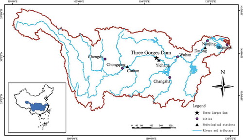
Before 2003, there were no major diversions or obstructions on the upstream reaches of the Yangtze River Basin (YRB) and, to the best of our knowledge, the streamflow values are not notably impacted by control structures (Xu et al. 2007). After 2003, with the construction of the TGD, the streamflow values, especially flood data at the YHS, were greatly influenced by the TGD. As a result, the streamflow data for the YHS after 2003 were adjusted to approximate natural flow, to keep the long-term records consistent by the principle of water balance. We collected the inflow, Q_i, and outflow, Q_o, of the TGD from the China Three Gorges Corporation¹ for the period after 2003. Let the observed streamflow at the Yichang site be Q_y, then the streamflow of the Yangtze River between the TGD and Yichang station is Q_y − Q_o; and this was added to the inflow of the TGD, Q_i. Finally, we replaced the observed streamflow after 2003 at the YHS by the adjusted streamflow (Q_y − Q_o + Q_i). The adjusted streamflow can serve as a practical estimate of natural streamflow at the YHS. The whole dataset (1953–2013) was used for subsequent FFA.

Flood peak (maximum annual daily discharge) and maximum annual 15-day volume were selected as the targets to analyse the joint distribution between flood elements. The day when maximum annual daily streamflow occurs must be located in the 15 days of maximum annual 15-day volume, ensuring that the flood peak and maximum annual 15-day volume are selected from the same flood in a given year. The Spearman correlation coefficient between flood peak and flood volume is 0.771, indicating that they are closely related and one cannot ignore the relationship in the FFA.

Candidate climate indices include 74 climate circulation parameters obtained from the China National Climate Center² and nine commonly used global climate indices: in terms of the Atlantic Ocean (North Atlantic Oscillation, NAO), the Pacific Ocean (North Pacific Index, NP; Eastern Pacific Oscillation, EPO; Pacific Decadal Oscillation, PDO), and three datasets of sea surface temperature, SST: Niño 3, Niño 3.4 and Niño 4). Details of these datasets are given in Table 1. The 74 climate circulation parameters include climate indices for the polar vortex in the Northern Hemisphere, the subtropical ridge over India, the subtropical ridge over the South China Sea, and the subtropical ridge over the Pacific, which have been used recently for meteorological or hydrological research in China (Zhang et al. 2017, Zhi-Yao et al. 2017). A polar vortex is an upper-level low-pressure area lying near the Earth’s poles. Some researchers have found an interaction between the polar vortex and outbreaks of severe cold, Arctic sea ice decline, reduced snow cover, evapotranspiration patterns, NAO anomalies, or weather anomalies in the Northern Hemisphere (e.g. Baldwin and Dunkerton 2001, Song and Robinson 2004, Overland 2013). The subtropical ridge, also known as the subtropical high, is a significant belt of atmospheric high pressure situated around the latitudes of 30°N in the Northern Hemisphere and 30°S in the Southern Hemisphere. It is a product of the global air circulation cell known as the Hadley Cell (Oliver 2005). As the subtropical ridge varies in position and strength, it can enhance or depress monsoon regimes around their low-latitude periphery (Wu et al. 2004).

Table 1. Candidate climate indices used in the study.

Climate index	Abbreviation	Source organization and associated website
74 circulation parameters		National Climate Center http://www.ncc-cma.net/cn/
North Atlantic Oscillation	NAO	Climatic Research Unit, University of East Anglia http://www.cru.uea.ac.uk/
North Pacific Index	NP	Climate Data Guide https://climatedataguide.ucar.edu/
Eastern Pacific Oscillation	EPO	NOAA ESRL Physical Sciences Division https://www.esrl.noaa.gov/psd/
Pacific Decadal Oscillation	PDO	Joint Institute for the Study of the Atmosphere and Ocean http://www.jisao.washington.edu/
Averaged SST for 5°S–5°N and 150–90°W	Niño 3	NOAA ESRL Physical Sciences Division https://www.esrl.noaa.gov/psd/
Averaged SST for 5°S–5°N and 170–120°W	Niño 3.4	NOAA ESRL Physical Sciences Division https://www.esrl.noaa.gov/psd/
Averaged SST for 5°S–5°N and 160°E–150°W	Niño 4	NOAA ESRL Physical Sciences Division https://www.esrl.noaa.gov/psd/
Pacific/North American pattern	PNA	Climate Prediction Center http://www.cpc.noaa.gov/
Northern Oscillation Index	NOI	Pacific Fisheries Environmental Laboratory http://www.pfeg.noaa.gov/

Identification of the climate covariates

Here, the climate indices were identified to find the explanatory covariates ($c_{1,i}$ and $c_{2,i}$) for subsequent GAMLSS-based prior distributions. The optimal number of covariates was determined to be two by referencing some similar studies (Steinschneider and Brown 2012, Liu et al. 2014, Lima et al. 2015, Zeng et al. 2017). Some studies have shown that the flood peak at the YHS during the flood season is influenced by ENSO (Dai and Wigley 2000, Xu et al. 2007). During the ENSO warm events, the East Asian monsoon circulation is weakened, causing less rainfall in northern China, leading to increased rainfall, streamflow and flooding in south central China, because the subtropical ridge remains to the south (Wu et al. 2004, Xu et al. 2007). Meanwhile, the Southern Oscillation Index (SOI) is closely related to ENSO. The SOI in April of the forecast year has a maximum Spearman correlation of −0.264 with the flood peak in the TGD for the preceding two years, and thus was selected as the first covariate for flood peak. Besides, the cold-air intrusion into China also influences precipitation in China (Wang et al. 2017). An index of the frequency of cold-air intrusions into China in April of the forecast year has a maximum Spearman coefficient of 0.419 for the preceding two years and was selected as the second covariate. The Spearman coefficient between the two covariates was 0.007, and they could therefore be regarded as independent.

The upper reaches of the YRB are located in the southwest region of China, subject to a subtropical monsoon climate. The precipitation in the YRB is influenced by the Indian subtropical ridge (Wu et al. 2004, Yang and Lau 2004, Xu et al. 2007, Zhou et al. 2011). The strength of the Indian subtropical ridge (65°E–95°E) in December of the antecedent year has a maximum Spearman coefficient of 0.259 for the preceding two years and was selected as the first covariate for flood volume. In addition, the polar vortex in the Northern Hemisphere has a great effect on the East Asian summer monsoon system and the rainfall in the YRB (Song et al. 2005). The index of the station of the polar vortex centre in the Northern Hemisphere in July of the antecedent year has a maximum Spearman coefficient of 0.350 for the preceding two years, and was therefore selected as the second covariate of flood volume. The Spearman coefficient between the two covariates was −0.111, so they were also almost independent.

Methods

Bayesian statistical methods were used to improve the GAMLSS-based prior distributions using the intrinsic relationship between flood peak and volume. Suppose x, y denote different flood elements, then the improved nonstationary model is expressed as:

(1) $f_i\left(x|y_i\right)=\frac{f(y_i|x)f_i\left(x\right)}{f_i\left(y_i\right)}$(1)

(2) $f_i\left(y_i\right)=\underset{-\mathrm{\infty }}{\overset{+\mathrm{\infty }}{\int }}f(y_i|x)f_i\left(x\right)\mathrm{d}x$(2)

where $f_i\left(x|y_i\right)$ is the posterior distribution of x in year i; $y_i$ is the observed predictand in year i, which gives the posterior information; $f(y_i|x)$ is the conditional probability distribution arising from the copula function; $f_i\left(x\right)$ is the GAMLSS-based prior distribution at year $i$; and $f_i\left(y_i\right)$ is the marginal density function of $y$ in year i when the variable $y$ is equal to $y_i$.

In this study, flood peak and flood volume were selected as targets, where x represents flood peak and y represents flood volume. The posterior distribution of flood peak was calculated. Then, the objects were reversed. The prior distribution $f_i\left(x\right)$ based on GAMLSS is described in Section ‘Prior distributions’, the conditional distribution $\left(y_i|x\right)$ derived from the copula distribution is shown in Section ‘Conditional probability function’, and the prediction of the $y_i$ is given in Section ‘Predictands’.

Prior distributions

The GAMLSS has been used successfully in nonstationary FFA (Liu et al. 2014, Lima et al. 2015, Zhang et al. 2015, Zeng et al. 2017) and was selected as the prior distribution herein, which assumes that the covariates and distribution parameters have linear or nonlinear association (Lane et al. 2005). The GEV distribution was selected to fit the distribution of flood peak and flood volume, as it has been used widely in hydrology and GAMLSS (Liu et al. 2014, Lima et al. 2015, Um et al. 2017). The GEV distribution contains three parameters: a location parameter, μ, a shape parameter, ξ, and a scale parameter, σ. According to previous studies (Liu et al. 2014, Lima et al. 2015, Kwon and Lall 2016), ξ and σ in this study were assumed to be invariant with time, while μ was taken as a nonstationary dependent variable with covariates. Then, the GLAMSS-based prior distribution $f_i\left(x\right)$ at year $i$ was as follows:

(3) $f_i\left(x\right)=\mathrm{G}\mathrm{E}\mathrm{V}\left({\mu }_i,\xi ,\sigma \right)$(3)

(4) ${\mu }_i=g\left(t,c_{1,i},c_{2,i},\alpha \right)$(4)

where t is the time covariate; $c_{1,i}$ and $c_{2,i}$ are the climate covariates (see Section ‘Identification of the climate covariates’); $\alpha$ represents the regression parameters that need to be estimated; and $g()$ is the function between μ_i and the covariates t$,c_{1,i}$and $c_{2,i}$. In this study, eight improved nonstationary models were established according to the different functions $g()$, which are listed in Table 2.

Table 2. Different functions $g()$ of the eight GAMLSS-based prior distributions used in the study.

Model	Function, $g()$
Model 1	${\mu }_i=a_0$
Model 2	${\mu }_i=a_0+a_{1}t$
Model 3	${\mu }_i=a_0+a_{1}t+a_2{t}^2$
Model 4	${\mu }_i=a_0+a_1{c}_{1,i}+a_2{c}_{2,i}$
Model 5	${\mu }_i=a_0+a_1{c}_{1,i}+a_2{c}_{2,i}+a_3{c}_{1,i}{c}_{2,i}$
Model 6	${\mu }_i=a_0+a_1{c}_{1,i}+a_2{c_{1,i}}^2+a_3{c}_{2,i}$
Model 7	${\mu }_i=a_0+a_1{c}_{1,i}+a_2{c}_{2,i}+a_3{c_{2,i}}^2$
Model 8	${\mu }_i=a_0+a_1{c}_{1,i}+a_2{c_{1,i}}^2+a_3{c}_{2,i}+a_4{c_{2,i}}^2$

The location parameter ${\mu }_i$ of Model 1 is constant, and the prior distribution 1 is the traditional stationary distribution; ${\mu }_i$ of Models 2 and 3 has linear and quadratic functions with the time covariates; and Models 4–8 consider linear or quadratic functions with $c_{1,i}$and $c_{2,i}$. The parameters of these eight models listed in Table 2 were estimated using the maximum likelihood (ML) method.

To sum up, three kinds of GAMLSS were considered in the prior distributions of eight models, including the stationary distribution (Model 1), time-informed nonstationary distributions (Models 2 3), and climate-informed nonstationary distributions (Models 4–8). These eight prior distributions can cover current GAMLSS distributions used for nonstationary FFA. Therefore, first we compared these eight prior distributions for nonstationary FFA and selected the best one for the TGD, and then the improvements of the proposed method to these eight prior distributions were evaluated.

Conditional probability function

The flood elements usually have an intrinsic relationship (Grimaldi and Serinaldi 2006, Mediero et al. 2010, Requena et al. 2013). It is necessary to consider the intrinsic relationship between flood peak and volume to inform the posterior distributions (e.g. the Spearman correlation coefficient between flood peak and flood volume of the TGD is 0.771). Due to the remarkable advances in the use of copula functions in hydrological research (Grimaldi and Serinaldi 2006, Zhang and Singh 2006, Renard and Lang 2007), a copula function was selected to fit the bivariate distributions, which may be expressed as follows:

(5) $F\left(x,y\right)=C\left(u,\mathrm{v}\right)$(5)

(6) $u=G\left(x\right),v=H\left(y\right)$(6)

where $C()$ is the copula function; $G\left(x\right)$ and $H\left(y\right)$ represent the cumulative density functions of $x$ and $y$, respectively; and $F()$ is the joint cumulative distribution between $x$ and $y$.

Based on the copula function, the conditional probability density function of a flood element may be expressed by Equation (7) (Grimaldi and Serinaldi 2006):

(7) $f\left(y|x\right)=\frac{f\left(x,y\right)}{g\left(x\right)}=\frac{\mathrm{d}C(G\left(x\right),H\left(y\right))}{\mathrm{d}x\mathrm{d}y}\times \frac{1}{g\left(x\right)}=\frac{\mathrm{d}C(G\left(x\right),H\left(y\right))}{\mathrm{d}G\left(x\right)\mathrm{d}H\left(y\right)}\times \frac{\mathrm{d}G\left(x\right)}{\mathrm{d}x}\times \frac{\mathrm{d}H\left(y\right)}{\mathrm{d}y}\times \frac{1}{g\left(x\right)}=\frac{\mathrm{d}C(G\left(x\right),H\left(y\right))}{\mathrm{d}G\left(x\right)\mathrm{d}H\left(y\right)}\times h\left(y\right)$(7)

In Equation (7) $g\left(x\right)$ and $h\left(\mathrm{y}\right)$ are the probability density functions of $x$ and $\mathrm{y}$, respectively; and $f\left(x,y\right)$ is the joint density function, which can be derived from the copula function.

Three commonly used copula functions, the Gumbel-Hougaard, Frank and Clayton copulas, were performed to fit the joint distributions between flood peak and volume based on (1) the maximum likelihood method (ML; Genest and Rivest 1993) and (2) the method-of-moments-like estimation (MOM; Genest et al. 1995, Reddy and Ganguli 2012). The MOM estimates the copula parameter $\theta$ using the one-to-one correspondence between $\theta$ and the Kendall correlation coefficient $\tau$. The probability distributions of copula functions and the relationships between $\theta$ and $\tau$ are shown in Table 3 (Nelsen 2006, Reddy and Ganguli 2012).

Table 3. Basic properties of the three copulas used in this study.

Copula	$C\left(u,v\right)$	Relationship with Kendall’s $\tau$
Gumbel-Hougaard	$\mathrm{e}\mathrm{x}\mathrm{p}\left\{-{\left({\left(-lnu\right)}^{\theta }+{\left(-lnv\right)}^{\theta }\right)}^{1/\theta }\right\}$	$\tau =\left(\theta -1\right)/\theta$
Clayton	${\left\{u^{-\theta }+v^{-\theta }-1\right\}}^{-1/\theta }$	$\tau =\theta /\left(\theta +2\right)$
Frank	$-\frac{1}{\theta }ln\left\{1+\frac{\left({\mathrm{e}}^{-\theta u}-1\right)\left({\mathrm{e}}^{-\theta v}-1\right)}{{\mathrm{e}}^{-\theta }-1}\right\}$	$\tau =1+\frac{4}{\theta }\left[\frac{1}{\theta }\underset{0}{\overset{\theta }{\int }}\frac{t}{e^t-1}\mathrm{d}t-1\right]$

Two criteria were selected to define the final copula function, the Akaike information criterion (AIC) and the Bayesian information criterion (BIC). The results are shown in Table 4.The Clayton copula determined using the ML method outperformed other copulas and was selected as the theoretical joint distribution function between flood peak and flood volume of the TGD. Then, the conditional distribution $f\left(y|x\right)$ could be derived from Equation (7).

Table 4. Parameters and AIC, BIC of copula functions. ML: maximum likelihood method; MOM: method-of-moments-like estimation. $\theta$: copula parameter; AIC: Akaike information criterion; BIC: Bayesian information criterion.

Candidate copula	Parameter estimation method	$\theta$	AIC	BIC
Gumbel-Hougaard	ML	2.186638	2530.002	2544.778
	MOM	2.458952	2531.232	2546.008
Frank	ML	3.155684	2498.527	2513.303
	MOM	2.917905	2498.779	2513.555
Clayton	ML	8.646803	2514.08	2528.856
	MOM	7.791	2514.606	2529.382

Predictands

After obtaining the prior distributions and the conditional probability function of flood elements, the marginal distribution of $y_i$ in Equation (1) still needed to be calculated. Therefore, a multiple linear regression model between flood elements and climate covariates was established. The climate indices in Table 1 from the preceding two years to April in the forecast year were selected as alternative predictors. The selection of predictors contains two steps. First, the Pearson correlation coefficients between climate predictors and flood peak and volume were calculated. The climate predictors whose Pearson coefficients relative to the flood elements were the highest 15 values were chosen to be the candidate predictors. Second, based on these 15 chosen candidate predictors, the “all subsets regression” method was used to select the final climate predictors based on adjusted R² using the “leap” package in R3.4.4 software.³ In the “all subsets regression” method, every possible model is inspected: the best one-predictor model is selected, followed by the best two-predictors model, the three-predictors model, up to a model with all 15 candidate predictors (Miller 2002). Finally, the predictors of the model with the largest adjusted R² are selected as the final predictors.

The final predictors used for prediction and their Pearson coefficients with flood elements are shown in Table 5. The climate indices in Table 5 are confirmed by some meteorological research on the YRB (Gong and Ho 2002, Xu et al. 2007, Qiang et al. 2013, Zhang et al. 2017) and are also consistent with the previous streamflow predictions in China (Xu et al. 2007, Qiang et al. 2013, Liu et al. 2014). The observed and predicted peak and volume of floods are shown in Figure 2. The Nash-Sutcliffe efficiency coefficient (Nash and Sutcliffe 1970) between observation and predictands was 0.676 and 0.601 for flood peak and flood volume, respectively. Thus, it is thought that the predictands $y_i$ are convincing.

Figure 2. Predictands of flood peak and flood volume for the period 1953–2013. The dashed (black) line is the observed value; the solid (blue) line is the predictand.

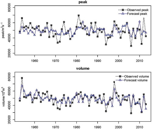
Table 5. Final climate covariates for flood peak and flood volume and their Pearson coefficients $p$ with flood elements.

Peak	$p$	Volume	p
① Index of the frequency of cold-air intrusion into China in April of the forecast year	0.413	① Index of the strength of the polar vortex centre in the Northern Hemisphere in December of the antecedent year	0.343
② Meridional index over Asia (60–150°E) in May of the forecast year	0.354	② Index of the strength of the subtropical ridge over North Africa, the Atlantic and North America (110°W–60°E) in December of the antecedent year	0.328
③ Index of the strength of the North African subtropical ridge (20°W–60°E) in March of the antecedent year	−0.326	③ Index of the northern extent of the North America–Atlantic subtropical ridge (110–20°W) in May of the antecedent two year	0.311
④ Index of the northern extent of the North America–Atlantic subtropical ridge (110–20°W) in July of the antecedent year	0.325	④ Index of the area of the subtropical ridge over the eastern Pacific (175–115°W) in September of the antecedent two years	0.308
⑤ Index of the area of the polar vortex in North America (120–30°W) in March of the antecedent two year	0.295	⑤ Index of the station of the polar vortex centre in the Northern Hemisphere in July of the antecedent year	0.303

Indices for model evaluation

The leave-one-out cross-validation method was used to reveal how well the Bayesian model can perform in truly out-of-sample predictions recognizing that different climate epochs may lead to different model performance (Chen et al. 2014, Thorarinsdottir et al. 2018). First, the first year is extracted, and the model is trained by the remaining years. Then, the posterior distribution of the first year is obtained based on the trained model. This process is then repeated for each year in the record until all predictive results are obtained. Finally, the model evaluation indices are calculated based on the results. In this paper, three indices were used to evaluate the prediction of flood peak and flood volume.

(1) The coefficient of efficiency, CE, which ranges from $-\mathrm{\infty }$ to +1, is similar to the statistic R² (Chen et al. 2014), and is given by:

(8) $\mathrm{C}\mathrm{E}=1-\frac{{\sum }_{i=1}^n{\left(O_i-S_i\right)}^2}{{\sum }_{i=1}^n{\left(O_i-O_c\right)}^2}$(8)

where $O_i$ and $S_i$ are, respectively, the observed values and the predicted posterior mean values of the flood elements in the year $i$, and $O_c$ is the mean value of the observed data. The CE is used to measure the goodness of fit of the model compared with the mean of the observed data; CE > 0 indicates that the predicted flood elements are better than the mean of the observed data, while CE < 0 indicates that the predictions are poorer than the mean of the observed data; in other words, the residual variance (described by the numerator in Equation (8)) is larger than the data variance (described by the denominator).

(2) Root mean square error of mean value, RMSEM. We refer to another commonly used index RMSE, and replace the predictands with the predicted posterior mean of the flood elements, then the RMSEM is defined as (Zeng et al. 2017):

(9) $\mathrm{R}\mathrm{M}\mathrm{S}\mathrm{E}\mathrm{M}=\sqrt{\frac{{\sum }_{i=1}^n{\left(O_i-S_i\right)}^2}{n}}$(9)

(3) Average band-width, AB. For a probability prediction, it is necessary to assess the uncertainty of the results. The AB was selected to represent the uncertainty of predictions (Xiong et al. 2009):

(10) $\mathrm{A}\mathrm{B}=\frac{1}{n}\sum _{i=1}^n\left(Q_i^{0.95}-Q_i^{0.05}\right)$(10)

where $Q_i^{0.95}$ and $Q_i^{0.05}$ are, respectively, the 0.95 and 0.05 quantiles of the result in year $i$. Therefore, AB represents the width of the 90% confidence interval. The smaller the AB, the better the prediction.

Results and discussions

Posterior distributions

The posterior distributions of eight models for flood peak and flood volume were calculated in this study. The evaluation indices of the eight models and their GAMLSS-based prior distributions are shown in Table 6. The improvement of all eight models was remarkable compared with their prior distributions. The CE values increased and the uncertainty parameters (AB) also declined in these eight models, indicating that the relationship between flood peak and flood volume could obviously improve GAMLSS-based prior distributions.

Table 6. Performance indices used for evaluating the performance of the eight models. CE: coefficient of efficiency; RMSEM: root mean square error of mean; AB: average band-width.

Flood element		Index	Model 1	Model 2	Model 3	Model 4	Model 5	Model 6	Model 7	Model 8
Peak	Prior distribution	CE	–0.036	–0.038	0.014	0.175	0.230	0.229	0.200	0.180
		RMSEM	8937.287	8942.337	8719.044	7975.218	7705.521	7706.872	7852.347	7951.692
		AB	29 109.870	29 168.710	30 453.670	25 850.250	26 041.750	25 201.850	25 860.950	25 185.750
	Posterior distribution	CE	0.242	0.190	0.203	0.355	0.393	0.377	0.361	0.340
		RMSEM	7644.610	7902.066	7836.732	7052.489	6837.970	6929.389	7017.287	7130.198
		AB	25 720.210	25 517.780	26 711.620	23 130.060	23 281.030	22 639.790	23 083.200	22 597.730
Volume	Prior distribution	CE	–0.046	–0.036	−0.088	0.218	0.232	0.287	0.208	0.296
		RMSEM	8789.316	8747.321	8964.565	7600.973	7530.565	7256.042	7649.529	7213.415
		AB	29 681.280	29 434.060	30 000.280	23 946.460	23 328.430	26 739.750	23 050.800	22 313.610
	Posterior distribution	CE	0.275	0.247	0.217	0.413	0.435	0.492	0.413	0.479
		RMSEM	7317.382	7459.847	7606.950	6583.274	6462.599	6128.806	6584.933	6206.965
		AB	26 041.100	25 990.610	26 366.260	21 391.440	20 768.280	23 401.980	20 989.630	20 401.970

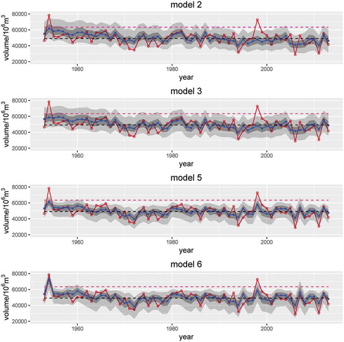
For flood peak estimation the optimal model was Model 5, and for flood volume estimation the optimal model was Model 6. Models 2 and 3 performed worst out of these eight models for flood peak and flood volume. The posterior distributions of Models 2, 3, 5 and 6 for flood peak and flood volume are plotted in Figures 3 and 4, respectively. In Figures 3 and 4, the uncertainty of Models 2 and 3 is larger than that of Models 5 and 6. The AB index also shows this phenomenon. In contrast, Models 5 and 6 performed much better and could describe some extreme floods. For example, there were extreme floods in the TGD in 1954 and 1998. The nonstationary flood volume of Models 2 and 3 was just equal to other ordinary years, whereas Model 6 could predict the extreme flood volume in these two years.

Figure 3. Posterior distributions of flood peak for Models 2, 3, 5 and 6. The solid (red) line is the observed flood peak; the shaded (grey) area is the 90% confidence interval, and the darker area is the 50% confidence interval; the solid lines are the 50% quantile (blue) and the dashed (red and black) lines represent the traditional 95% and 50% quantiles, respectively, under the stationarity assumption.

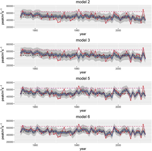
Figure 4. Posterior distributions of flood volume for Models 2, 3, 5 and 6. See Figure 3 for explanation.

Even though the prior distributions of these eight models are different, the conditional distribution used to obtain the posteriors of the eight models is the same; that is to say, they all used the same copula function to improve the GAMLSS-based prior distributions. Therefore, the different performance of these eight models may be mainly attributed to the GAMLSS-based prior distributions. Comparing prior distributions and posterior distributions, it was found that if the prior distribution performed better, then the posterior distributions would perform better too. Taking Model 2 as an example: the prior distribution performed worst compared with other prior distributions for flood peak, but the posterior distribution was also the worst of the eight models. Therefore, it is essential to choose an optimal nonstationary prior distribution as the prior distribution.

Influence on the dynamic management of TGD

The nonstationary model in this study used climate indices as covariates and can give results before the flood season occurs. Thus, the risks of coming floods are predicted and the managers of the TGD can receive information on these risks and adapt to the potential coming floods. As a result, the management of the TGD is dynamic and adapted to the risks of floods. The management of hydraulic projects based on nonstationary FFA is termed “dynamic management” in this paper. The results of Models 5 and 6 are used to discuss the influence of the nonstationary FFA on the dynamic management of the TGD due to their good performance for flood peak and flood volume out of the eight models.

The 1%, 5% and 10% design values were determined under stationary FFA, which is the prior distribution of Model 1. Then, the nonstationary exceedence probabilities of these design values were plotted, as shown in Figure 5. Under the stationary assumption, the exceedence probabilities were equal to 1%, 5% and 10% throughout. However, under the nonstationary assumption, the exceedence probabilities were less than 1%, 5% and 10% in most years and larger than these probabilities only in a few years, such as 1954 and 1998. Meanwhile, there were extreme floods in the TGD in 1954 and 1998. Therefore, if the nonstationary models were used for the management of the TGD, the exceedence probabilities would be much larger than those based on the stationary assumption when extreme floods occurred; so the risks of extreme floods would be reported as lower when compared to the stationary assumption.

From Figure 5, it can be seen that, when FFA evolves from stationarity to nonstationarity, the influence on the dynamic management of hydraulic engineering is significant. It is critical to propose a framework for dynamic management based on the nonstationary FFA to reduce the expected risks of some extreme floods. Meanwhile, given the studies of dynamic management based on short-term flood prediction (Xiang et al. 2010, Chen et al. 2013), dynamic management combining the short-term prediction and nonstationary FFA for certain hydraulic engineering projects, such as reservoirs, is a good choice for the future.

Figure 5. Nonstationary exceedence probabilities of stationary 1%, 5% and 10% design values, respectively, for (a, c, e) flood peak, and (b, d, f) flood volume. Dashed lines are the stationary exceedence probabilities, and the small circles are the nonstationary exceedence probabilities of stationary design values.

However, there are some flaws in nonstationary FFA that hamper the dynamic management of hydraulic projects. First, the choice of climate indices still needs further investigation. In this study, we selected climate indices based on previous studies and correlation coefficients. However, different researchers will have different criteria and may select different climate indices. As a result, the nonstationary FFA will be different. This difference will bring large uncertainty for dynamic management and is not allowed for management of some large hydraulic projects such as the TGD. Second, the reliability and robustness of nonstationary FFA need further investigation and improvement. The errors between nonstationary FFA and observed floods are smaller compared with stationary FFA, but are still large for dynamic management. The different nonstationary models used in this study can also produce entirely different results. For example, the nonstationary flood volume of Models 5 and 6 for 1954 is totally different, as shown in Figure 4. The error of Model 5 for flood volume in 1954 is too large and could bring danger for the TGD if the results of Model 5 were used.

Conclusions

In this paper, improved nonstationary models for flood peak and volume of the TGD were established by making use of the intrinsic relationship between flood elements. Then, the influence of the nonstationary assumption on the management of hydraulic engineering was analysed. The primary conclusions of this study can be summarized as follows:

Compared with the GAMLSS-based prior distributions, the improved model clearly increases the accuracy and reduces the uncertainty of the flood distribution. It will be a good choice to update prior nonstationary distributions by the intrinsic relationship between hydrological elements in the future.

The prior distributions of Models 1, 2 and 3 exhibited inferior performance compared with other GAMLSS-based prior distributions. The prior distributions that used climate indices as covariates gave the best performance and were much better than the others. In addition, the weaknesses of prior distributions can always make posterior distributions worse. Thus, it is necessary to select an optimal prior distribution in the improved nonstationary model.

The nonstationary FFA could be helpful for the dynamic management of hydraulic engineering. From the case study of the TGD, it is seen that the dynamic management strategies under the nonstationarity assumption are more secure and economical. It is important to propose a framework for dynamic management based on nonstationary FFA, especially in the context of climate change.

Disclosure statement

No potential conflict of interest was reported by the authors.

Additional information

Funding

This research was supported financially by the National Key R&D Programme of China [Grant no. 2016YFC0402708], the National Science Foundation of China [Grant nos. 51439007, 91647119, 91547205], the Innovation group of Hubei Natural Science Foundation [Grant no. 2017CFA015], and the Youth Innovation Promotion Association CAS [no. 2017074].

Notes

¹ http://www.ctg.com.cn/.

² http://ncc.cma.gov.cn.

³ https://cran.r-project.org/web/packages/leaps/.

References

- Aghakouchak, A., et al., 2013. Extremes in a changing climate. Trends in Antarctic Terrestrial & Limnetic Ecosystems, 65 (10), 954.
- Ahn, K.H. and Palmer, R.N., 2016. Use of a nonstationary copula to predict future bivariate low flow frequency in the Connecticut £river £basin. Hydrological Processes, 30 (19), 3518–3532. doi:10.1002/hyp.10876
- Baldwin, M.P. and Dunkerton, T.J., 2001. Stratospheric harbingers of anomalous weather regimes. Science, 294 (5542), 581–584. doi:10.1126/science.1063315
- Bender, J., Wahl, T., and Jensen, J., 2014. Multivariate design in the presence of non-stationarity. Journal of Hydrology, 514, 123–130. doi:10.1016/j.jhydrol.2014.04.017
- Bracken, C., et al. 2018. A Bayesian hierarchical approach to multivariate nonstationary hydrologic frequency analysis. Water Resources Research, 54 (1), 377–384. doi:10.1002/2017WR020403
- Callau Poduje, A.C., Belli, A., and Haberlandt, U., 2014. Dam risk assessment based on univariate versus bivariate statistical approaches: A case study for Argentina. Hydrological Sciences Journal, 59 (12), 2216–2232. doi:10.1080/02626667.2013.871014
- Chen, J., et al. 2013. Joint operation and dynamic control of flood limiting water levels for cascade reservoirs. Water Resources Management, 27 (3), 749–763. doi:10.1007/s11269-012-0213-z
- Chen, X., et al. 2014. Climate information based streamflow and rainfall forecasts for Huai River Basin using hierarchical Bayesian modeling. Hydrology and Earth System Sciences, 18 (4), 1539–1548. doi:10.5194/hess-18-1539-2014
- Cunderlik, J.M., et al. 2007. Local non-stationary flood-duration-frequency modelling. Canadian Water Resources Journal, 32 (1), 43–58. doi:10.4296/cwrj3201043
- Dai, A. and Wigley, T.M.L., 2000. Global patterns of ENSO-induced precipitation. Geophysical Research Letters, 27 (9), 1283–1286. doi:10.1029/1999GL011140
- Dai, Z.J., et al. 2010. Assessment of extreme drought and human interference on baseflow of the Yangtze River. Hydrological Processes, 24 (6), 749–757. doi:10.1002/hyp.7505
- Debele, S.E., Strupczewski, W.G., and Bogdanowicz, E., 2017. A comparison of three approaches to non-stationary flood frequency analysis. Acta Geophysica, 65 (4), 863–883. doi:10.1007/s11600-017-0071-4
- García, J.A., et al. 2018. A Bayesian hierarchical spatio-temporal model for extreme rainfall in Extremadura (Spain). Hydrological Sciences Journal, 63 (6), 878–894. doi:10.1080/02626667.2018.1457219
- Genest, C., Ghoudi, K., and Rivest, L.P., 1995. A semiparametric estimation procedure of dependence parameters in multivariate families of distributions. Biometrika, 82 (3), 543–552. doi:10.1093/biomet/82.3.543
- Genest, C. and Rivest, L.P., 1993. Statistical inference procedures for bivariate Archimedean copulas. Publications of the American Statistical Association, 88 (423), 1034–1043. doi:10.1080/01621459.1993.10476372
- Gershunov, A. and Cayan, D.R., 2003. Heavy daily precipitation frequency over the contiguous United States: sources of climatic variability and seasonal predictability. Journal of Climate, 16 (16), 2752–2765. doi:10.1175/1520-0442(2003)016<2752:HDPFOT>2.0.CO;2
- Gong, D.Y. and Ho, C.H., 2002. Shift in the summer rainfall over the Yangtze River valley in the late 1970s. Geophysical Research Letters, 29 (10), 78–88. doi:10.1029/2001GL014523
- Grimaldi, S. and Serinaldi, F., 2006. Asymmetric copula in multivariate flood frequency analysis. Advances in Water Resources, 29 (8), 1155–1167. doi:10.1016/j.advwatres.2005.09.005
- Gu, X., et al. 2017. Nonstationarity-based evaluation of flood risk in the Pearl River basin: changing patterns, causes and implications. Hydrological Sciences Journal, 62 (2), 246–258. doi:10.1080/02626667.2016.1183774
- Guo, H., et al., 2012. Effects of the Three Gorges Dam on Yangtze River flow and river interaction with Poyang Lake, China: 2003–2008. Journal of Hydrology, 416, 19–27. doi:10.1016/j.jhydrol.2011.11.027
- Haylock, M.R., et al. 2006. Trends in total and extreme South American rainfall in 1960–2000 and links with sea surface temperature. Journal of Climate, 19 (8), 1490–1512. doi:10.1175/JCLI3695.1
- Henley, B.J., et al., 2011. Climate-informed stochastic hydrological modeling: incorporating decadal-scale variability using paleo data. Water Resources Research, 47, W11509. doi:10.1029/2010WR010034
- Jiang, C., et al. 2015. Bivariate frequency analysis of nonstationary low-flow series based on the time-varying copula. Hydrological Processes, 29 (6), 1521–1534. doi:10.1002/hyp.10288
- Kwon, H.H., Brown, C., and Lall, U., 2008. Climate informed flood frequency analysis and prediction in Montana using hierarchical Bayesian modeling. Geophysical Research Letters, 35 (5), L05404. doi:10.1029/2007GL032220
- Kwon, H.H., et al. 2009. Seasonal and annual maximum streamflow forecasting using climate information: application to the Three Gorges Dam in the Yangtze River basin, china. Hydrological Sciences Journal, 54 (3), 582–595. doi:10.1623/hysj.54.3.582
- Kwon, H.H. and Lall, U., 2016. A copula-based nonstationary frequency analysis for the 2012–2015 drought in California. Water Resources Research, 52 (7), 5662–5675. doi:10.1002/2016WR018959
- Lane, P.W., et al. 2005. Generalized additive models for location, scale and shape – discussion. Applied Statistics, 54, 544–554.
- Li, J., et al. 2018. Nonstationary flood frequency analysis for annual flood peak and volume series in both univariate and bivariate domain. Water Resources Management, 32 (13), 4239–4252. doi:10.1007/s11269-018-2041-2
- Lima, C.H.R., et al., 2015. A climate informed model for nonstationary flood risk prediction: application to Negro River at Manaus, Amazonia. Journal of Hydrology, 522, 594–602. doi:10.1016/j.jhydrol.2015.01.009
- Liu, D., et al. 2014. Climate-informed low-flow frequency analysis using nonstationary modelling. Hydrological Processes, 29 (9), 2112–2124. doi:10.1002/hyp.10360
- Mediero, L., Jimenez-Alvarez, A., and Garrote, L., 2010. Design flood hydrographs from the relationship between flood peak and volume. Hydrology and Earth System Sciences, 14 (12), 2495–2505. doi:10.5194/hess-14-2495-2010
- Miller, A., 2002. Subset selection in regression. 2nd. New York: Chapman and Hall.
- Milly, P., et al. 2008. Stationarity is dead. Science, 319 (5863), 573–574. doi:10.1126/science.1151915
- Milly, P.C.D., et al., 2015. On critiques of “Stationarity is dead: whither water management”. Water Resources Research. doi:10.1002/2015WR017408
- Nash, J.E. and Sutcliffe, J.V., 1970. River flow forecasting through conceptual models part 1 — a discussion of principles. Journal of Hydrology, 10 (3), 282–290. doi:10.1016/0022-1694(70)90255-6
- Nelsen, R.B., 2006. An introduction to copulas. New York: Springer.
- Oliver, J.E., 2005. Hadley cell. In: J.E. Oliver, ed.. Encyclopedia of world climatology. Dordrecht: Springer Netherlands, 398.
- Overland, J.E., 2013. Atmospheric science: long-range linkage. Nature Climate Change, 4 (1), 11–12. doi:10.1038/nclimate2079
- Qiang, A., et al. 2013. Research on the changes of local weather and climate in the three gorges reservoir. Disaster Advances, 6, 498–504.
- Reddy, M.J. and Ganguli, P., 2012. Bivariate flood frequency analysis of Upper Godavari River flows using Archimedean copulas. Water Resources Management, 26 (14), 3995–4018. doi:10.1007/s11269-012-0124-z
- Renard, B., 2011. A Bayesian hierarchical approach to regional frequency analysis. Water Resources Research, 47 (11), 602–610. doi:10.1029/2010WR010089
- Renard, B. and Lang, M., 2007. Use of a Gaussian copula for multivariate extreme value analysis: some case studies in hydrology. Advances in Water Resources, 30 (4), 897–912. doi:10.1016/j.advwatres.2006.08.001
- Requena, A.I., Mediero, L., and Garrote, L., 2013. A bivariate return period based on copulas for hydrologic dam design: accounting for reservoir routing in risk estimation. Hydrology and Earth System Sciences, 17 (8), 3023–3038. doi:10.5194/hess-17-3023-2013
- Salas, J.D. and Obeysekera, J., 2014. Revisiting the concepts of return period and risk for nonstationary hydrologic extreme events. Journal of Hydrologic Engineering, 19 (3), 554–568. doi:10.1061/(ASCE)HE.1943-5584.0000820
- Song, C., et al. 2005. The relation between Yichang drought and climate atmospheric circulation ed. The volume of papers of Chinese Meteorological Society in 2005. (in Chinese).
- Song, Y. and Robinson, W.A., 2004. Dynamical mechanisms for stratospheric influences on the troposphere. Journal of the Atmospheric Sciences, 61 (14), 1711–1725. doi:10.1175/1520-0469(2004)061<1711:DMFSIO>2.0.CO;2
- Steinschneider, S. and Brown, C., 2012. Forecast-informed low-flow frequency analysis in a Bayesian framework for the northeastern United States. Water Resources Research, 48 (10), 18132–18137. doi:10.1029/2012WR011860
- Strupczewski, W.G., et al. 2016. Comparison of two nonstationary flood frequency analysis methods within the context of the variable regime in the representative polish rivers. Acta Geophysica, 64 (1), 206–236. doi:10.1515/acgeo-2015-0070
- Strupczewski, W.G., et al., 2009. On seasonal approach to nonstationary flood frequency analysis. Physics & Chemistry of the Earth Parts A/B/C, 34(10-12), 612–618. doi:10.1016/j.pce.2008.10.067
- Sun, S., et al. 2017. A Bayesian method for missing rainfall estimation using a conceptual rainfall–runoff model. Hydrological Sciences Journal, 62 (15), 2456–2468. doi:10.1080/02626667.2017.1390317
- Sun, X., et al., 2014. A general regional frequency analysis framework for quantifying local-scale climate effects: A case study of ENSO effects on southeast Queensland rainfall. Journal of Hydrology, 512, 53–68. doi:10.1016/j.jhydrol.2014.02.025
- Thorarinsdottir, T.L., et al. 2018. Bayesian regional flood frequency analysis for large catchments. Water Resources Research, 54 (9), 6929–6947. doi:10.1029/2017WR022460
- Um, M.-J., et al. 2017. Modeling nonstationary extreme value distributions with nonlinear functions: an application using multiple precipitation projections for U.S. cities. Journal of Hydrology, 552 (Supplement C), 396–406. doi:10.1016/j.jhydrol.2017.07.007
- Villarini, G., et al. 2009. Flood frequency analysis for nonstationary annual peak records in an urban drainage basin. Advances in Water Resources, 32 (8), 1255–1266. doi:10.1016/j.advwatres.2009.05.003
- Volpi, E. and Fiori, A., 2012. Design event selection in bivariate hydrological frequency analysis. Hydrological Sciences Journal, 57 (8), 1506–1515. doi:10.1080/02626667.2012.726357
- Wang, C., et al. 2017. Analysis of rainstorm induced by interaction between typhoon Chan-hom (2015) and cold air in northeast China. Plateau Meteorology, 36 (5), 1257–1566.
- Willems, P., 2013. Adjustment of extreme rainfall statistics accounting for multidecadal climate oscillations. Journal of Hydrology, 490, 126–133. doi:10.1016/j.jhydrol.2013.03.034
- Wu, M.C., Chang, W.L., and Leung, W.M., 2004. Impacts of El Niño Southern Oscillation events on tropical cyclone landfalling activity in the western north pacific. Journal of Climate, 17 (6), 1419–1428. doi:10.1175/1520-0442(2004)017<1419:IOENOE>2.0.CO;2
- Xiang, L., et al. 2010. Dynamic control of flood limited water level for reservoir operation by considering inflow uncertainty. Journal of Hydrology, 391 (1), 124–132. doi:10.1016/j.jhydrol.2010.07.011
- Xiong, L.H., et al. 2009. Indices for assessing the prediction bounds of hydrological models and application by generalized likelihood uncertainty estimation. Hydrological Sciences Journal, 54 (5), 852–871. doi:10.1623/hysj.54.5.852
- Xu, K.Q., et al. 2007. Climate teleconnections to Yangtze River seasonal streamflow at the Three Gorges Dam, China. International Journal of Climatology, 27 (6), 771–780. doi:10.1002/joc.1437
- Yang, F.L. and Lau, K.M., 2004. Trend and variability of china precipitation in spring and summer: linkage to sea-surface temperatures. International Journal of Climatology, 24 (13), 1625–1644. doi:10.1002/joc.1094
- Yang, Y.P., et al. 2017. Influence of large reservoir operation on water-levels and flows in reaches below dam: case study of the Three Gorges Reservoir. Scientific Reports, 7, 14.
- Zeng, H., et al. 2017. Nonstationary extreme flood/rainfall frequency analysis informed by large-scale oceanic fields for Xidayang Reservoir in North China. International Journal of Climatology, 37 (10), 3810–3820. doi:10.1002/joc.4955
- Zhang, L. and Singh, V.P., 2006. Bivariate flood frequency analysis using the copula method. Journal of Hydrologic Engineering, 11 (2), 150–164. doi:10.1061/(ASCE)1084-0699(2006)11:2(150)
- Zhang, Q., et al., 2015. Evaluation of flood frequency under non-stationarity resulting from climate indices and reservoir indices in the East River Basin, China. Journal of Hydrology, 527, 565–575. doi:10.1016/j.jhydrol.2015.05.029
- Zhang, Y.Q., et al. 2017. Spatio-temporal characteristics and possible mechanisms of rainy season precipitation in Poyang Lake Basin, China. Climate Research, 72 (2), 129–140. doi:10.3354/cr01455
- Zhi-Yao, H.E., et al., 2017. Annual average runoff ensemble forecast for Jinping I-stage hydropower station based on Elman neural network. Water Resources & Power, 35 (10), 25–28.
- Zhou, M., et al. 2011. Insights from a joint analysis of Indian and Chinese monsoon rainfall data. Hydrology and Earth System Sciences, 15 (8), 2709–2715. doi:10.5194/hess-15-2709-2011