A two-stage fuzzy-stochastic factorial analysis method for characterizing effects of uncertainties in hydrological modelling

ABSTRACT

In this study, a two-stage fuzzy-stochastic factorial analysis (TFFA) method is developed and applied to the Vakhsh watershed (upper reaches of Aral Sea basin, Central Asia) for daily streamflow simulation. TFFA has advantages in identifying the major parameters that have important individual and interactive effects on model outputs, as well as assessing multiple uncertainties resulting from randomness and vagueness characteristics of model parameters. The results reveal that (a) nine major parameters (from a total of 24) have significant effects on Soil Water Assessment Tool (SWAT) simulation performance for the study watershed; and (b) snowmelt-related parameters (including snowfall temperature, threshold temperature for snowmelt and s nowmelt factor) and runoff curve number (CN2) are most sensitive parameters for the runoff generation. The results also show that the proposed TFFA method can help enhance the hydrological model’s capability for runoff simulation/prediction, particularly for in data-scarce and high-mountainous watersheds.

KEYWORDS:

• Central Asia
• fuzzy sets
• Markov Chain Monte Carlo (MCMC)
• SWAT
• two-stage factorial analysis
• uncertainty effects

Editor A. Fiori;Associate editor R. Singh

1 Introduction

Hydrological models are useful tools for operational applications, such as water resource management, flooding control and hydropower generation, as well as scientific research to understand hydrological processes (Li et al. 2017a, Remesan et al. 2018, Tegegne et al. 2019). Hydrological models usually contain a large number of parameters to represent complex hydrological cycles and watershed/basin system characteristics (Behrouz et al. 2020). These parameters must be estimated through a calibration process before the implementation of a hydrological model. The estimation of model parameters contains significant uncertainties, which may be attributed to over-parameterization of the model structure, correlation among parameters, vagueness of feasible ranges and the spatiotemporal heterogeneity of a hydrological system. Ignoring these uncertainties can lead to complex calibration processes and waste of computing resources, as well as potentially yield biased and misleading results (Fan et al. 2016, Gan et al. 2018, Ahmadi et al., 2019). In particular, the scarcity of data in many regions (e.g. Central Asia) may further intensify the complexity of a hydrological modelling system, resulting in poor parameter identifiability. In response to such complexities and uncertainties, more robust uncertainty analysis approaches are desired for facilitating reliable hydrological simulation/prediction.

In the past, many research works have been conducted for uncertainty assessment in hydrological models. For example, Abbaspour et al. (2015) implemented the Sequential Uncertainly Fitting (SUFI-2) method to calibrate a continental-scale hydrological model based on the Soil and Water Assessment Tool (SWAT) for Europe. Han and Zheng (2018) conducted the uncertainty analysis of a SWAT model through coupling Markov Chain Monte Carlo (MCMC) and Bayesian Model Averaging (BMA). Their results showed that the Bayesian-based method provides an efficient way to identify the uncertainty characteristics of model parameter and structure. Ahmadi et al. (2019) proposed a fuzzy general regression neural network (FGRNN) to evaluate the parameter uncertainty in a hydrological model and their results showed that fuzzy logic-based methods were ideal means to deal with the uncertainty of a hydrological model system. Tran and Kim (2019) coupled the Generalized Likelihood Uncertainty Estimation (GLUE) model and polynomial chaos expansion to assess the parameter uncertainty for a lumped hydrological model in the Thu Bon basin, Vietnam. Lee et al. (2020) compared the simulation performance of three modelling structures for the SWAT model in the Choptank River watershed, USA, where BMA was employed to evaluate the structural uncertainty in the SWAT model. In general, these previous studies focused on quantifying parameter uncertainties in hydrological modelling. For instance, MCMC is effective for drawing the posterior distributions of uncertain parameters based on Bayesian statistical inference. However, many hydrological models with the detailed structure are controlled by a large number of parameters, which may result in complex calibration processes and a waste of computing resources. In addition, different parameter combinations may lead to equifinality, which is defined as multiple parameter sets with equally acceptable calibration and validation results which potentially yields greater parameter uncertainties (Enrique et al. 2014, Arsenault and Brissette 2015, Kelleher et al. 2017). Thus, it is imperative to assess the effects/implications of hydrological parameters on model outputs and identify the major parameters that exert the most influence on the performance of model simulation.

Factorial analysis (FA), as an attractive variance-based sensitivity analysis method, is useful for quantifying the impacts of hydrological parameters on model outputs and assessing potential inter-relationships among uncertain parameters. Previously, FA was widely used in biochemical areas and environmental modelling systems due to its easy implementation and effectiveness (Panic et al. 2015, Wang et al. 2015, El-Helaly et al. 2018). However, since the number of model runs required for a FA experiment increases exponentially with the number of parameters, the conventional FA has rarely been employed in more complex hydrological simulation (e.g. SWAT). Thus, a two-stage factorial analysis (TFA) method is advanced to overcome this limitation. TFA contains a prerequisite step to screen out important parameters and an in-depth analysis stage to provide good information about the individual and interactive relationships among multiple parameters. However, the feasible ranges of hydrological parameters are often accompanied by various complexities (e.g. errors of input data, spatiotemporal heterogeneity of hydrological systems and watershed characteristics) and there is not sufficient information to represent these ambiguous characteristics. Fuzzy set analysis (FSA) is helpful for dealing with the vagueness of parameters and is based on fuzzy set theory, which has the advantage of directly handling uncertain parameters without generating a large number of samples (Li et al. 2019). Therefore, a potential approach for effectively identifying the major parameters and their interactions on model outputs is to incorporate FSA within a factorial analysis framework.

The Aral Sea (in Central Asia), once the fourth largest lake in the world, has shrunk sharply since the 1960s due to a combination of the consumption of water for agricultural irrigation, the construction of hydropower infrastructure and climate change (Shen et al. 2019). The decline of water flow in the Aral Sea basin (i.e. the Syr Darya and Amu Darya rivers) brings severe eco-environmental problems, such as vegetation degradation, soil salinization and agricultural drought (Cretaux et al. 2013). Thus, accurately modelling the hydrological conditions in the Aral Sea is urgent to support water resource management and ensure eco-environmental sustainability, especially in the upper reaches of these rivers. The SWAT model, as a typical process-based hydrological model, can not only achieve the reliable hydrological simulation/prediction, but also provide the physical description of hydrological processes (Krysanova and White 2015). Unfortunately, due to both a lack of data and the high elevation of the upper reaches, few previous studies have been conducted to model hydrological processes and analyse the relationships between model parameters and watershed characteristics through the SWAT model in the Aral Sea area.

Therefore, the objective of this study is to develop a two-stage fuzzy-stochastic factorial analysis (TFFA) method through incorporating the techniques of TFA, FSA and MCMC into a general framework. The main novelty and contribution of this study are as follows:

1. an innovative method of TFFA is developed for assessing parameter uncertainties in hydrological modelling;

2. TFFA is shown to be effective for screening out important parameters and investigating the individual and interactive effects of multiple parameters on model responses;

3. TFFA is used to reflect the vagueness and randomness characteristics of hydrological parameters with FSA and Bayesian inference;

4. TFFA is applied to the SWAT model of the Vakhsh watershed in Central Asia, a high-mountain watershed with a lack of data; and

5. multiple parameter sets under different feasible ranges are analysed, which can facilitate the understanding of watershed hydrological processes, especially in the data-scarce watershed.

This paper is organized as follows: Section 2 presents the development of TFFA method; Section 3 describes the study area, data acquisition and hydrological model set-up; Section 4 presents the results and discussion, and Section 5 draws main conclusions and potential extensions of the proposed method.

2 Methodology

Figure 1 shows the general framework of TFFA, which involves three main procedures: (a) simulating watershed rainfall–runoff processes through SWAT; (b) assessing the effects of individual and interactive parameters on model outputs based on TFA and FSA; and (c) quantifying the uncertainties of parameters through MCMC.

Figure 1. Schematic of the two-stage fuzzy-stochastic factorial analysis (TFFA) method.

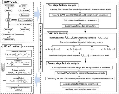
The SWAT model is used for simulating daily rainfall–runoff processes; it is a physically based semi-distributed hydrological model operating on a daily/monthly time step (Malago et al. 2018, Brighenti et al. 2019). SWAT is controlled by a large number of parameters, such as runoff curve number (CN2), soil hydraulic conductivity (SOL_K) and snowfall temperature (SFTMP). Factorial analysis derived from design of experiment (DOE), is an effective multivariate inference method for quantifying the individual and interactive effects of parameters on model response. The FA processes used in SWAT can be summarized as: (i) setting up the running table of factorial design for uncertain parameters (e.g. CN2, SOL_K and SFTMP); (ii) running the hydrological model according to the table to obtain the corresponding model responses; (iii) calculating the standardized effect of parameters and multi-parameter interactions; and (iv) identifying the important/sensitive parameters for the hydrological model. Since the number of model runs required for the FA experiment increases exponentially with the number of parameters, the full factorial design has rarely been employed in more complex hydrological simulators (e.g. SWAT).

A two-stage factorial analysis (TFA) method is proposed based on Plackett-Burman design and $2_R^{k-p}$ design. In this process, the parameters (CN2, SOL_K and SFTMP) are called factors and the output variables (i.e. simulated runoff) are called responses. The first stage is a Plackett-Burman design experiment, which is conducted for screening out important/sensitive parameters. The second stage is a series of $2_R^{k-p}$ design experiments, which are employed to explore both individual and interactive impacts of selected parameters, as follows (Montgomery 2012):

(1) $E_i=\frac{\mathrm{C}\mathrm{o}\mathrm{n}\mathrm{t}\mathrm{r}\mathrm{a}\mathrm{s}{\mathrm{t}}_i}{2^{k-p-1}}$(1)

(2) $\mathrm{S}{\mathrm{S}}_i=\frac{{\left(\mathrm{C}\mathrm{o}\mathrm{n}\mathrm{t}\mathrm{r}\mathrm{a}\mathrm{s}{\mathrm{t}}_i\right)}^2}{2^{k-p}}$(2)

where E_i is the standardized effect of factor i or multi-factor interaction; Contrast_i is calculated by using plus and minus signs in column i of Yates’ order table; and SS_i is the sum of squares for factor i or multi-factor interaction. Details on the theoretical background and methodology of Plackett-Burman design and $2_R^{k-p}$ design can be found in Montgomery (2012).

In the TFA processes, the feasible ranges of model parameters (CN2, SOL_K and SFTMP) are often surrounded with vagueness and ambiguity due to insufficient information to represent the watershed characteristics. FSA is used for dealing with the vagueness of parameters and is based on fuzzy set theory. A fuzzy parameter number ${\tilde{\theta }}_n$ with continuous membership function can be expressed as (Bortolan and Degani 1985):

(3) ${\mu }_{\tilde{\theta }}\left(x\right)=\left\{\begin{array}{c}{f}_{\tilde{\theta }}\left(x\right)if{\theta }_n^{-}\le x\le d_n^{-}\\ 1if{d}_n^{-}\le x\le d_n^{+}\\ g_{\tilde{\theta }}\left(x\right)if{d}_n^{+}\le x\le {\theta }_n^{+}\\ 0\mathrm{o}\mathrm{t}\mathrm{h}\mathrm{e}\mathrm{r}\mathrm{w}\mathrm{i}\mathrm{s}\mathrm{e}\end{array}\right.$(3)

where ${\theta }_n^{-}$, $d_n^{-}$, $d_n^{+}$, ${\theta }_n^{+}$ ∈ R and ${\theta }_n^{-}\le d_n^{-}\le d_n^{+}\le {\theta }_n^{+}$; $f_{\tilde{\theta }}\left(x\right)$ and $g_{\tilde{\theta }}\left(x\right)$ are a continuously and monotonically increasing function and decreasing function, respectively. The interval $\left[{\theta }_n^{-},{\theta }_n^{+}\right]$ represents the initial ranges of fuzzy parameter ${\tilde{\theta }}_n$. A trapezoidal fuzzy number can be converted into a group of intervals associated with multiple α-cut levels and the possibility ranges of parameters can be represented as follows (Yager 1999):

(4) ${\tilde{\theta }}_n\left(\alpha \right)=\begin{array}{c}\{0\le \alpha \le 1\left|\alpha d_n^{-}+\left(1-\alpha \right){\theta }_n^{-}\le {\theta }_n\le \alpha d_n^{+}\right.\\ +\left(1-\alpha \right){\theta }_n^{+}\}\end{array}$(4)

Then, the intervals $\left[{\theta }_n^{-}\left(\alpha \right),{\theta }_n^{+}\left(\alpha \right)\right]$ under different α-cut levels from all fuzzy sets can be obtained. In this study, the different combinations of intervals of hydrological parameters are used as inputs of the TFA experiments. After screening out the most sensitive parameters through TFA, the randomness characteristics of hydrological parameters are assessed through MCMC approach. Implementation of the MCMC method is dependent on the principles of Bayesian inference (Vrugt et al. 2008):

(5) $p\left(\theta \left|Y_{\mathrm{o}\mathrm{b}\mathrm{s}}\right.\right)=\frac{p\left(\theta \right)\cdot p\left(Y_{\mathrm{o}\mathrm{b}\mathrm{s}}|\theta \right)}{p\left(Y_{\mathrm{o}\mathrm{b}\mathrm{s}}\right)}$(5)

where p(θ) is the prior distribution of the model parameter; p(θ|Y_obs) is the posterior distribution of the model parameter; p(Y_obs|θ) is the likelihood function; and p(Y_obs) represents marginal likelihood and is not required in practice. The statistical inferences of p(θ|Y_obs) can then be formulated as (Vrugt et al. 2008):

(6) $p\left(\theta \left|Y_{\mathrm{o}\mathrm{b}\mathrm{s}}\right.\right)\propto p\left(\theta \right)\cdot p\left(Y_{\mathrm{o}\mathrm{b}\mathrm{s}}|\theta \right)$(6)

In this study, the simulation errors are assumed to have independent Gaussian distribution; then, the likelihood function is provided as follows:

(7) $p\left(Y_{\mathrm{o}\mathrm{b}\mathrm{s}}|\theta \right)={\prod }_{t=1}^n\frac{1}{\sqrt{2\pi }}\mathrm{e}\mathrm{x}\mathrm{p}\left(-\frac{{\left(y_t-y_{\mathrm{o}\mathrm{b}\mathrm{s},t}\right)}^2}{2{\sigma }_e^2}\right)$(7)

Nevertheless, it is difficult to obtain the calculated or analytical posterior distributions of parameters because of the nonlinear and complicated structure of hydrological models. Based on Bayesian inference, MCMC methods provide a simple and efficient way to sample the posterior distribution from a Markov chain. In this study, the DREAM (DiffeRential Evolution Adaptive Metropolis) algorithm is conducted to infer the posterior distributions; this is an effective MCMC sampler and has been widely used for model optimization and uncertainty quantification in hydrological modelling (Leta et al. 2015, Sun et al. 2017). The Nash-Sutcliffe model efficiency (E_NS) and Kling-Gupta efficiency (KGE) are used for goodness-of-fit testing of the model simulation; these are defined as follows (Nash and Sutcliffe 1970, Gupta et al. 2009):

(8) $E_{\mathrm{N}\mathrm{S}}=1-\frac{{\sum }_{i=1}^n{\left(H_{\mathrm{o}\mathrm{b}\mathrm{s},i}-H_{\mathrm{s}\mathrm{i}\mathrm{m},i}\right)}^2}{{\sum }_{i=1}^n{\left(H_{\mathrm{o}\mathrm{b}\mathrm{s},i}-{\bar{H}}_{\mathrm{o}\mathrm{b}\mathrm{s}}\right)}^2}$(8)

(9) $\mathrm{K}\mathrm{G}\mathrm{E}=1-\sqrt{{\left(\alpha -1\right)}^2+{\left(\beta -1\right)}^2+{\left(\gamma -1\right)}^2}$(9)

(10) $\alpha ={\sigma }_{\mathrm{s}\mathrm{i}\mathrm{m}}/{\sigma }_{\mathrm{o}\mathrm{b}\mathrm{s}}$(10)

(11) $\beta =\left({\mu }_{\mathrm{s}\mathrm{i}\mathrm{m}}-{\mu }_{\mathrm{o}\mathrm{b}\mathrm{s}}\right)/{\sigma }_{\mathrm{o}\mathrm{b}\mathrm{s}}$(11)

(12) $\gamma =\frac{\mathrm{c}\mathrm{o}\mathrm{v}\left(H_{\mathrm{s}\mathrm{i}\mathrm{m},i},H_{\mathrm{s}\mathrm{i}\mathrm{m},i}\right)}{{\sigma }_{\mathrm{s}\mathrm{i}\mathrm{m}}\cdot {\sigma }_{\mathrm{o}\mathrm{b}\mathrm{s}}}$(12)

where H_obs,i and H_sim,i are, respectively, the observed and simulated values on day i; n is the number of simulated days; ^―H_obs is the average observed value; μ_obs and μ_sims are the means of observed and simulated values, respectively; and σ_obs and σ_sims are the standard deviation of observed and simulated values, respectively. Values of ENS and KGE close to 1 indicate that the better calibration/validation is achieved.

3 Case study

3.1 Study area

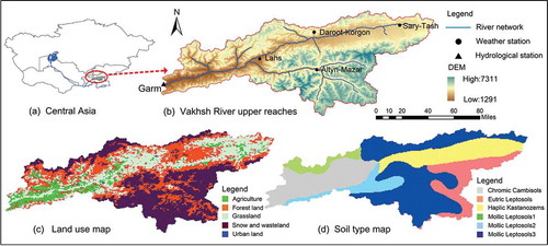
The Vakhsh watershed in Central Asia is chosen as the study area (Fig. 2), which is located between 38°66′N–39°86′N and 70°28′E–73°71′E. The elevation of the Vakhsh River varies from 1291 to 7311 m a.s.l. and the catchment area above Garm station is 19 638 km². The average annual precipitation for the study watershed in the period 1979–1986 is 1506 mm/year, and the average minimum and maximum temperatures are – 9.9°C and 0.7°C, respectively. Forest land (31%), grassland (21%), snow and wasteland (35%) are the main vegetation types in the watershed. Mollic leptosols (50%), chromic cambisols (17%), haplic kastanozems (19%) and eutric leptosols (14%) are the major soil types. The Vakhsh River is one of the main tributaries of Amu Darya River, with a length of 524 km, and originates from the Pamir-Alai Mountains (Kai et al. 2007). The Amu Darya River follows a gradient from the mountains to the plains and from east to west; the annual precipitation in this river basin is less than 100 mm/year in the plains and about 1000–2000 mm in the mountains (Jiang et al. 2017). For this reason, the mountain ranges are a very important source of water in the Amu Darya River basin and runoff is mainly fed by melting snows and glaciers (Lee and Jung 2018). The effective hydrological modelling is desired to facilitate the local water resource management. However, few modelling studies have focused on the hydrological processes in the Amu Darya River, especially in the upper reaches of the watershed, which are mountainous and have a very important contribution to the river flow.

Figure 2. Location and spatial data in Vakhsh watershed for the SWAT model: (a) position of the studied watershed; (b) DEM and position of the gauging stations; (c) land-use map; and (d) soil type map.

3.2 Data acquisition and model set-up

The data requirement for SWAT modelling primarily includes spatial data (i.e. DEM, soil types and land-use map), geological characteristic data (i.e. soil and land-use properties) and hydro-meteorological data (i.e. rainfall, air temperature, wind speed, solar radiation, relative humidity and daily runoff data). As shown in Fig. 2, digital elevation model (DEM) data with 90-m resolution were obtained from the Consortium on Spatial Information of Consultative Group on International Agricultural Research (CGIAR¹). Land-use maps (1990) with 1-km resolution were obtained from the Global Land Cover Facility (GLCF²) and land-use properties (e.g. agriculture land, forest land and grass land) were directly obtained from the SWAT model database. A soil type map and soil properties were derived from the Harmonized World Soil Database.³ For the meteorological data, precipitation and air temperature were observed at four meteorological stations (Sary-Tash, Daroot-Korgon, Lahs and Altyn-Mazar) in the Vakhsh catchment for the period 1979–1986. Daily runoff data (Garm hydrometric station) for the Vakhsh River were acquired from the Global Runoff Data Centre (GRDC⁴), and included discharge data for the period 1979–1986, which was used for calibration and validation of the model.

For the model set-up, the ArcSWAT 2012 interface is conducted to parameterize the processes of hydrological simulation. Based on the DEM map, the watershed is divided into 25 sub-watersheds, which are further subdivided into 91 hydrological response units (HRUs). The calibration period is from 1981 to 1984, where the first two years are a burn-in period for initialization and the validation period is from 1985 to 1986. The 24 parameters related to surface runoff simulation are evaluated by the proposed method and the descriptions of these parameters are shown in Table 1.

Table 1. Description of model parameters and their initial ranges.

Category	Parameter ^a	Description	Initial range
Groundwater	v__GW_DELAY	Groundwater delay (d)	[0, 500]
	v__ALPHA_BF	Baseflow recession constant (d)	[0, 1]
	v__GWQMN	Threshold depth of water in the shallow aquifer required for return flow to occur (mm)	[0, 2000]
	v__GW_REVAP	Groundwater revap coefficient	[0.02, 0.2]
	v__REVAPMN	Threshold depth of water in the shallow aquifer for revap (mm)	[0, 500]
	v__RCHRG_DP	Deep aquifer percolation fraction	[0, 1]
Surface runoff	r__CN2	Initial SCS runoff curve number to moisture condition II	[−0.6, 0.2]
	v__SURLAG	Surface runoff lag time	[1, 24]
Soil water	r__SOL_Z	Depth from soil surface to bottom of layer (mm)	[−0.99, 5]
	r__SOL_BD	Soil bulk density (g/cm^3)	[−0.5, 0.5]
	r__SOL_AWC	Available water capacity of the soil layer	[−0.99, 5]
	r__SOL_K	Soil hydraulic conductivity (mm/d)	[−0.99, 5]
	r__SOL_ALB	Moist soil albedo	[−0.99, 5]
Main channel	v__CH_N2	Manning’s n value for the main channel	[0, 0.3]
	v__CH_K2	Effective hydraulic conductivity of channel (mm/h)	[0, 500]
Evapotranspiration	v__ESCO	Soil evaporation compensation factor	[0, 1]
	v__EPCO	Plant uptake compensation factor	[0, 1]
Snow water	v__SFTMP	Snowfall temperature (°C)	[−10, 10]
	v__SMTMP	Snow melt base temperature (°C)	[−10, 10]
	v__SMFMX	Melt factor for snow on June 21 (mm/°C)	[0, 20]
	v__SMFMN	Melt factor for snow on December 21 (mm/°C)	[0, 20]
	v__TIMP	Snowpack temperature lag factor	[0, 1]
	v__SNOCOVMX	Minimum snow water content corresponding to 100% snow cover	[0, 500]
	v__SNO50COV	Fraction of snow volume corresponding to 50% snow cover	[0, 1]

^av_ and ‘r_ represent a replacement and a relative change to the original parameter values, respectively.

4 Results and discussion

4.1 Screening main parameters

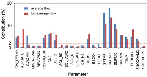
After running SWAT in a total of 28 treatment combinations of a Plackett-Burman design, the main effects of the 24 parameters on model responses (i.e. average flow and log-average flow) are obtained. The main effects are calculated as the difference between the average responses of each parameter made at a high level and a low level. Figure 3 presents the contributions of individual parameters to average flow and log-average flow, and those with a contribution of either average flow or log-average flow larger than 2% are defined as important parameters. From the results, the following 14 parameters have important effects on model responses: GW_DELAY, ALPHA_BF, GWQMN, RCHRG_DP, CN2, SOL_Z, CH_K2, SFTMP, SMTMP, SMFMX, SMFMN, TIMP, SURLAG and SNOCOVMX. The main limitation of the Plackett-Burman design is its incapability of reflecting interactive effects among multiple parameters; it can only reflect the main effects of parameters. More importantly, it has a complex alias structure and main effects may be partially aliased with some interactions (Phoa et al. 2009). Therefore, an in-depth analysis of important parameters is desired to make a clear test of main effects and interactions.

Figure 3. Contribution of individual parameters to modelling responses (24 parameters).

4.2 Effects of parameters

To further identify the relationships between parameters, a $2_{\mathrm{V}\mathrm{I}}^{14-5}$ fractional factorial design is conducted to identify both individual and interactive effects of uncertain parameters on model responses, where 14 is the number of parameters and 5 indicates the 1/2⁵ fraction of the 2¹⁴ full factorial design. The vagueness of feasible range is expressed by fuzzy sets and their fuzzy intervals based on trapezoidal membership function are illustrated in Fig. 4. The intervals [${\theta }_n^{-}$,${\theta }_n^{+}$] are defined by the initial ranges of parameters and the intervals [$d_n^{-}$,$d_n^{+}$] are obtained from the modellers’ experience. The parameter numbers and the two levels of each parameter under four α-cut levels (i.e. 0.25, 0.5, 0.75, 1) are presented in Table 2.

Table 2. Levels of factors for the 2¹⁴⁻⁵ experiment design.

Parameter number	Parameter	Factor level	α-cut levels
			0.25	0.5	0.75	1
1	v__GW_DELAY	Low	25	50	75	100
		High	475	450	425	400
2	v__ALPHA_BF	Low	0.05	0.1	0.15	0.2
		High	0.95	0.9	0.85	0.8
3	v__GWQMN	Low	100	200	300	400
		High	1900	1800	1700	1600
4	v__RCHRG_DP	Low	0.05	0.1	0.15	0.2
		High	0.95	0.9	0.85	0.8
5	r__CN2	Low	–0.54	–0.48	–0.42	–0.36
		High	0.18	0.16	0.14	0.12
6	r__SOL_Z	Low	–0.891	–0.792	–0.693	–0.594
		High	4.5	4	3.5	3
7	v__CH_K2	Low	25	50	75	100
		High	475	450	425	400
8	v__SFTMP	Low	–9	–8	–7	–6
		High	9	8	7	6
9	v__SMTMP	Low	–9	–8	–7	–6
		High	9	8	7	6
10	v__SMFMX	Low	1	2	3	4
		High	19	18	17	16
11	v__SMFMN	Low	1	2	3	4
		High	19	18	17	16
12	v__TIMP	Low	0.05	0.1	0.15	0.2
		High	0.95	0.9	0.85	0.8
13	v__SURLAG	Low	2.15	3.3	4.45	5.6
		High	22.85	21.7	20.55	19.4
14	v__SNOCOVMX	Low	2.15	50	75	100
		High	25	450	425	400

Figure 4. Fuzzy intervals based on trapezoidal membership function (14 parameters).

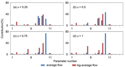
After running the SWAT model for a total of 512 treatment combinations for each α-cut level, the individual and interactive effects of uncertain parameters on model response (i.e. the average flow and log-average flow) can be identified. Figure 5 illustrates the individual contributions of 14 parameters for the model responses, including average flow and log-average flow. From the results, three snowmelt-related parameters (SFTMP, SMTMP, SMFMX and SMFMN) are seen to have important influence on the model responses. The importance of the snowmelt-related parameters is mainly because snow and glaciers are widely distributed in the Vakhsh watershed and snowmelt runoff is an important contributor to streamflow in the ablation period (Armstrong et al. 2018). In addition, three groundwater-related parameters (GW_DELAY, ALPHA_BF and RCHRG_DP), one surface runoff-related parameter (CN2) and one channel-related parameter (CH_K2) have obvious effects on model responses. The results show that streamflow generation in the study watershed is controlled by different hydrological processes (percolation, groundwater recharge and the transmission losses of the river channel). In addition, the contribution of parameters to average flow and log-average flow is different. This is because of the considerable differences between the values of high and low runoff in the study watershed and the response of log-average flow is mainly used to emphasize the baseflow (Cheng et al. 2014). There are several important hydrological processes affecting baseflow in the Vakhsh watershed, including rainfall runoff during summer, groundwater recharge and main channel transmission losses.

Figure 5. Contribution of individual parameters to modelling responses (14 parameters).

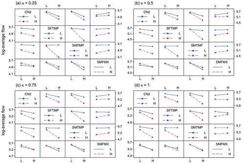
Figures 6 and 7 show the effects of individual parameters on model responses (average flow and log-average flow) under different α-cut levels. If the slope of the line is positive, there is a positive effect of the parameter on model response; and the steeper the slope, the greater the effect on model response. From the results, three parameters (SMFMX, SMFMN and CN2) have obviously positive effects and two parameters (SFTMP and SMTMP) have obviously negative effects on average flow. Parameters SMFMX and SMFMN are the snowmelt factor for 21 June and 21 December, respectively, and these control the speed rate of snowmelt. The positive effects are mainly because a higher rate of snowmelt would result in a greater amount of snowmelt runoff. Parameter CN2 is the initial runoff curve number, which relates to the potential of runoff generation. The positive effect of CN2 is because the rainfall in the spring and summer can cause infiltration and saturation excess runoff and thus result in an increase in average flow. Parameter SFTMP is snowfall temperature, which is used to categorize precipitation as rainfall or snowfall and has a significant negative effect on average flow. This is mainly because higher snowfall temperature leads to a smaller amount of snowfall, which would further decrease the generation of snowmelt runoff. Parameter SMTMP, which is the threshold temperature for snowmelt and controls the process of snowpack accumulation, has a significant negative impact on average flow. This is because a high SMTMP value leads to a high amount of snowpack accumulation, which would further result in the decrease of snowmelt runoff.

Figure 6. Main effect plots on modelling responses (α = 0.25 and α = 0.5).

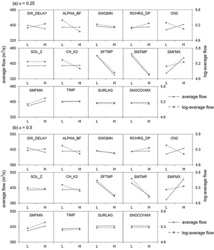
Figure 7. Main effect plots on modelling responses (α = 0.75 and α = 1).

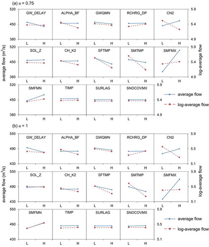
For log-average flow, four parameters (GW_DELAY, RCHRG_DP, SMFMX and SMFMN) have obviously positive effects and five parameters (ALPHA_BF, CN2, CH_K2, SFTMP and SMTMP) have obviously negative effects. It is noted from the results that some parameters (GW_DELAY, RCHRG_DP, ALPHA_BF and CH_K2) have important effects on log-average flow that is used to emphasize the baseflow, but little effect on average flow. Parameter GW_DELAY is the groundwater delay time and RCHRG_DP is the deep aquifer percolation fraction. The negative effects of these two parameters on baseflow are mainly because they control the processes of groundwater recharge and higher GW_DELAY and RCHRG_DP would increase the groundwater recharge to baseflow. Parameter CH_K2 is the effective hydraulic conductivity of the main channel, which has an important negative effect on baseflow. This is because CH_K2 controls the main channel transmission losses and higher CH_K2 values would increase the loss of baseflow with a constant loss rate in the main channel. Parameter ALPHA_BF represents the baseflow recession constant, which has a significant effect on baseflow but no obvious effect on peak flow. This is because ALPHA_BF controls the recharge of groundwater flow and higher ALPHA_BF values would result in the fast recharge of groundwater flow. The average flow is the mean value of daily discharge, which is highly influenced by peak flow. The lesser effects of GW_DELAY, RCHRG_DP, ALPHA_BF and CH_K2 on average flow may due to the fact that the processes of groundwater recharge and channel transmission losses are important contributors to baseflow and not sensitive to peak flow.

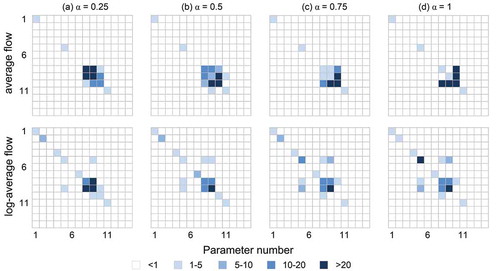
Two-factor interactions are also revealed by the $2_{\mathrm{V}\mathrm{I}}^{14-5}$ fractional factorial designs, which demonstrate some important model processes and especially how one process affects another. Figure 8 presents the individual and interactive contributions of 14 parameters to model responses under each α-cut level. The parameter numbers in the x- and y-axes are shown in Table 2. The results indicate that SFTMP, SMTMP, SMFMX and SMFMN have a lot of interactive effects on average flow. This is mainly because snowmelt runoff volume is abundant in the ablation period, leading to higher impacts of snowmelt-related parameters. The different processes of snow water movement controlled by these parameters mean that they would be interacting with each other. For example, the volume of snowfall controlled by SFTMP would affect the amount of snowpack accumulation controlled by SMTMP. For log-average flow, CN2, SFTMP, SMTMP and SMFMX have a lot of interactive effects, mainly because CN2 relates to the potential of runoff generation, which has important effects on the baseflow. In fact, both rainfall and snowmelt have important effects on the streamflow of the Vakhsh River, where the baseflow is dominated by the processes of snowmelt as well as infiltration excess and saturated excess mechanisms.

Figure 8. Individual and interactive contributions of 14 parameters to modelling responses under each α-cut level.

To further understand how the parameter interactions would affect the model responses, Figs. 9 and 10 present the interaction plots of uncertain parameters. These plots reveal the effect of one parameter on model output under the influence of another parameter: large differences in slope indicate there are greater interactive effects of two parameters on model responses. Parallel lines indicate there is no influence on model responses of parameter interactions.

Figure 9. Interactive plots for average flow response.

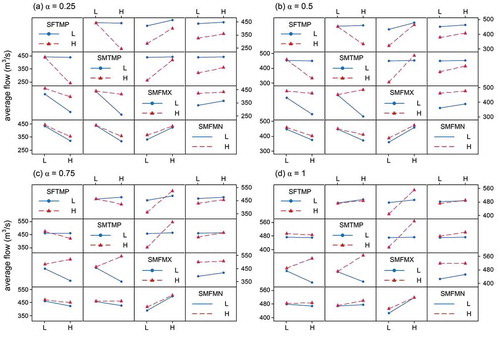
Figure 10. Interactive plots for log-average flow response.

Figure 9 presents the interaction plots of four parameters (SFTMP, SMTMP, SMFMX and SMFMN) for average flow under each α-cut level. In detail, when SFTMP is at the high level, SMTMP would have a higher negative effect on average flow. This is because both SFTMP and SMTMP have significant effects on the processes of snowmelt runoff. The high value of SFTMP leads to more precipitation being categorize as snowfall, which can increase the effects of snowmelt threshold temperature represented by SMTMP. Similarly, when SMTMP is high, SMFMX would have a higher positive effect on average flow. This is mainly because a higher SMTMP would lead to increased snowpack accumulation and thus increase the effect of snowmelt speed represented by SMFMX.

Figure 10 presents the interaction plots of four parameters (CN2, SFTMP, SMTMP and SMFMX) for log-average flow under each α-cut level. In comparison, the effects of SFTMP, SMTMP and SMFMX are large, while CN2 is fixed at the high level and small when CN2 is at the low level. This is because the high level of the initial runoff curve number would improve the potential of runoff generation and thus influence the effect of other parameters including threshold temperature for snowmelt, snowfall temperature and snowmelt factor.

4.3 Uncertainty analysis

Based on the results of both individual and interactive effects, nine parameters are selected for model calibration and uncertainty analysis based on MCMC; these are GW_DELAY, ALPHA_BF, RCHRG_DP, CN2, SFTMP, SMTMP, SMFMX and SMFMN. In this study, an effective MCMC algorithm named DREAM was used for inferring the parameters’ posterior distributions. For the DREAM algorithm parameterization, prior distributions of model parameters are assumed to be uniform distribution within their initial ranges and eight Markov chains are selected with 50 000 iterations for each one, leading to 400 000 model simulations. The first 50% of samples in each Markov chain are excluded as a burn-in period and the mean acceptance rate is 18.2%. The convergence criterion of $\hat{R}$ = 1.2 is often realized within 16 000 iterations for each Markov chain. The posterior distributions of parameters are obtained based on 20 000 parameter sets sampled after $\hat{R}$ convergence. For efficient model evaluation, given our computer resources (an Intel Core i7-6700 CPU 3.40 GHz processor), 10 000 iterations of eight Markov chains with nine parameters require about 4 hours to finish. However, when 24 parameters are all within the evaluation of the DREAM algorithm, the 10 000 iterations would require more than 12 hours. Moreover, evaluation with 24 parameters would result in over-parameterization of the hydrological model and would make the Markov chains difficult to converge.

Figure 11 presents the histograms of the posterior distribution of the parameters at the initial ranges (α-cut = 0). Compared with their initial ranges, all parameter ranges occur in relatively small intervals. The distribution of some parameters (GW_DELAY, ALPHA_BF, CN2, CH_K2, SFTMP, SMTMP and SMFMX) is approximately normal, while the distribution of RCHRG_DP largely concentrates on the upper bound and is negatively skewed. Parameter RCHRG_DP is the aquifer percolation coefficient that controls the amount of water moving into the deep aquifer; its negatively skewed distribution shows that the recharge of the deep aquifer in the Vakhsh watershed is very high. In addition, the distribution of SMFMN is largely concentrated on the lower bound and is positively skewed. Parameter SMFMN, representing melt factor on 21 December, can affect the speed of snowmelt; its posterior distribution shows that the snowmelt speed for the winter is slow in the study watershed. Table 3 presents a summary of the basic statistics (mean, standard deviation, as well as the 2.5th, 50th and 97.5th percentiles) of the posterior pdfs of the nine parameters. The 95PCI values of some parameters (RCHRG_DP, SFTMP, SMTMP, SMFMX and SMFMN) appear in quite narrow ranges, while other parameters (GW_DELAY, ALPHA_BF, CN2, CH_K2) show considerably wider ranges, indicating that the latter contain more uncertainties.

Table 3. Summarizing the basic statistics of the posterior pdfs of nine parameters. SD: standard deviation.

Parameter	Mean	SD	2.5th percentile	50th percentile	97.5th percentile
v_GW_DELAY	308.0	37.6	281.9	305.7	332.9
v_ALPHA_BF	0.361	0.0221	0.344	0.359	0.374
v_RCHRG_DP	0.986	0.0120	0.979	0.989	0.996
r_CN2	–0.392	0.0412	–0.419	–0.389	–0.364
v_CH_K2	177.3	18.9	163.4	170.8	188.4
v_SFTMP	0.0267	0.0499	–0.0129	0.0336	0.0694
v_SMTMP	9.39	0.180	9.28	9.39	9.49
v_SMFMX	2.75	0.204	2.62	2.74	2.86
v_SMFMN	0.132	0.122	0.0428	0.0982	0.188

Figure 11. Posterior pdfs of the parameters at different α-cut levels.

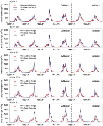
To further investigate how the vagueness of feasible ranges affected the performance of uncertainty analysis and model simulation, Fig. 11 presents histograms of the posterior distributions of the parameters at different α-cut levels. All parameter values are well identified and different from their initial ranges. The parameters SFTMP, SMFMX and SMFMN remain at their upper or lower bounds. From these results, quite different parameter values are obtained when the vagueness characteristics of the parameter ranges are considered. Figure 12 illustrates the observed and simulated daily discharge in calibration and validation periods under different α-cut levels, as well as the 95PCI of simulated discharge. The performance results of the hydrological model, evaluated based on E_NS and KGE for the calibration (1981–1984) and validation (1985–1986) periods, are presented in Table 4. According to the definition, the values of α, β and γ measure, respectively, the relative variability, bias and linear correlation between the simulated and observed values. The best calibration performance occurs under α-cut = 0 with E_NS and KGE of 0.918 and 1.049, respectively; and the best validation performance occurs under α-cut = 0.5 with E_NS and KGE of 0.762 and 1.004, respectively. The results show that nine parameters (GW_DELAY, ALPHA_BF, RCHRG_DP, CN2, SFTMP, SMTMP, SMFMX and SMFMN) out of 24 are needed to adequately capture the total model variance. Poor simulation performances occur under α-cut = 0.15 and 1, which do not capture the magnitude of high discharge events well. The model performance appears to decrease with the rise in α-cut level. This is due to the fact that a higher α-cut level is associated with a reduced interval of feasible range of the parameters; a wider feasible range can result in better calibration performance. However, the best validation performance is given by α-cut = 0.5, indicating that the parameter sets with better performance in the calibration period may not ensure the better performance in the validation period. The nonuniformity of model performance between calibration and validation periods may be attributed to systematic and random errors of input data, over-fitting in the calibration process, nonstationarity of streamflow and imperfection of objective function (Gupta et al. 2009).

Table 4. Model performance indicators at different α-cut levels. E_NS: Nash-Sutcliffe efficiency; KGE: Kling-Gupta efficiency; α, β and γ: respectively, the relative variability, bias and linear correlation between the simulated and observed values.

Period	α-cut level	ENS	KGE	α	β	γ
Calibration	0	0.918	1.049	1.021	–0.048	0.961
	0.25	0.911	1.054	1.035	–0.052	0.959
	0.5	0.672	1.171	1.151	–0.155	0.878
	0.75	0.613	1.163	1.205	–0.137	0.865
	1	0.369	1.076	1.328	–0.005	0.803
Validation	0	0.743	0.774	1.282	0.280	0.961
	0.25	0.664	0.750	1.333	0.329	0.956
	0.5	0.762	1.004	1.214	0.022	0.921
	0.75	0.675	1.125	1.182	–0.104	0.881
	1	0.337	0.769	1.394	0.355	0.863

Figure 12. Observed discharge (red triangle), simulated discharge at the maximum of the posterior pdfs (blue line) and the 95% confidence intervals of daily discharge (grey area) at different α-cut levels.

5 Conclusions

In this study, a two-stage fuzzy-stochastic factorial analysis (TFFA) method was developed for assessing parameter uncertainty in a hydrological model. The TFFA incorporates two-stage factorial analysis (TFA), fuzzy set analysis (FSA), Markov Chain Monte Carlo (MCMC) and Soil Water Assessment Tool (SWAT) within a general framework. TFFA can help (a) identify the major parameters that have important individual and interactive effects on model outputs; and (b) assess the multiple uncertainties resulting from randomness and vagueness characteristics of model parameters. The developed method is applied to the Vakhsh watershed (the upper reaches of the Aral Sea basin, Central Asia) for daily streamflow simulation. A total of 2048 factorial experiments were designed for examining the impacts of parameter uncertainty on model performance. Several findings are summarized below:

Nine major parameters (i.e. GW_DELAY, ALPHA_BF, RCHRG_DP, CN2, SFTMP, SMTMP, SMFMX and SMFMN) of a total of 24 are identified, which is sufficient for model parameterization and plays an important role in model performance and uncertainty quantification.

Snowmelt-related parameters (SFTMP, SMTMP, SMFMX and SMFMN), which represent snowfall temperature, threshold temperature for snowmelt and snowmelt factor for 21 June and 21 December, respectively, have important effects on average flow and baseflow. This implies that snowmelt runoff is an important contributor to streamflow for the Vakhsh watershed, where the snow and glaciers are widely distributed.

Parameter CN2, which relates to the potential of runoff generation, has a large effect on average flow and baseflow. This implies that the summer rainfall in the study watershed can cause infiltration and saturation excess runoff, which is an important contributor to streamflow in the study watershed.

The parameters GW_DELAY, RCHRG_DP, ALPHA_BF and CH_K2, which represent groundwater delay time, deep aquifer percolation fraction, baseflow recession constant and effective hydraulic conductivity of the main channel, respectively, have important effects on baseflow, but no obvious effects on average flow. This implies that the processes of groundwater recharge and channel transmission losses are important contributors to baseflow.

The parameters SFTMP, SMTMP, SMFMX and SMFMN have important interactions on average flow, implying that the different processes of snow water movement controlled by these parameters affect each other.

The vague nature of the parameter ranges has an important effect on model performance and uncertainty quantification; a lower α-cut level associated with a larger feasible parameter range could result in better model performance. These findings can help to specify the inter-relationships among the uncertain parameters and thus help to enhance the model’s applicability.

The feasibility of TFFA is demonstrated by assessing parameter uncertainty of the SWAT model in the Vakhsh watershed, Central Asia. The results indicate that multiple uncertainties, including over-parameterization of the model structure and the randomness and vagueness characteristics of model parameters, can be handled effectively. However, there are also some potential extensions of the proposed method. For example, from the results, some observation of high discharge events failed to be well captured; this may be the result of input and calibration data errors, as well as model structural imperfections. Although both parameter uncertainties and their effects on model responses are addressed through TFFA, input data errors and model structural uncertainties need to be explored in the future study. Secondly, this study used only one hydrological model (i.e. SWAT) to demonstrate the feasibility of TFFA. Additional research should include other hydrological models (e.g. HBV, VIC and TOPMODEL) to provide an ensemble simulation of water cycle processes in the Vakhsh watershed and analyse their parameter effects on model responses. Finally, compared with other uncertainty analysis methods (e.g. Bayesian model averaging), TFFA cannot obtain an aggregated simulation from multiple parameter sets and model structure. Therefore, the proposed TFFA method should be further improved through introducing other advanced uncertainty analysis algorithms that can handle these complexities.

Acknowledgements

The authors are grateful to the editors and the anonymous reviewers for their insightful comments and suggestions.

Disclosure statement

No potential conflict of interest was reported by the authors.

Additional information

Funding

This research was supported by the Strategic Priority Research Program of the Chinese Academy of Sciences [Grant no. XDA20060302].

Notes

¹ http://srtm.csi.cgiar.org.

² http://glcf.umd.edu.

³ https://daac.ornl.gov/.

⁴ https://www.bafg.de.

References

- Abbaspour, K.C., et al., 2015. A continental-scale hydrology and water quality model for Europe: calibration and uncertainty of a high-resolution large-scale swat model. Journal of Hydrology, 524, 733–752. doi:10.1016/j.jhydrol.2015.03.027
- Ahmadi, A., Nasseri, M., and Solomatine, D.P., 2019. Parametric uncertainty assessment of hydrological models: coupling UNEEC-P and a fuzzy general regression neural network. Hydrological Sciences Journal, 64 (9), 1080–1094. doi:10.1080/02626667.2019.1610565
- Armstrong, R.L., et al., 2018. Runoff from glacier ice and seasonal snow in high Asia: separating melt water sources in river flow. Regional Environmental Change, 19, 1249–1261. doi:10.1007/s10113-018-1429-0
- Arsenault, R. and Brissette, F.P., 2015. Continuous streamflow prediction in ungauged basins: the effects of equifinality and parameter set selection on uncertainty in regionalization approaches. Water Resources Research, 50, 6135–6153. doi:10.1002/2013WR014898
- Behrouz, M.S., et al., 2020. A new tool for automatic calibration of the Storm Water Management Model (SWMM). Journal of Hydrology, 581, 124436. doi:10.1016/j.jhydrol.2019.124436
- Bortolan, G. and Degani, R., 1985. A review of some methods for ranking fuzzy subsets. Fuzzy Sets and Systems, 15 (1), 1–19. doi:10.1016/0165-0114(85)90012-0
- Brighenti, T.M., et al., 2019. Simulating sub-daily hydrological process with SWAT: a review. Hydrological Sciences Journal, 64 (12), 1415–1423. doi:10.1080/02626667.2019.1642477
- Cheng, Q.B., et al., 2014. Improvement and comparison of likelihood functions for model calibration and parameter uncertainty analysis within a Markov Chain Monte Carlo scheme. Journal of Hydrology, 519, 2202–2214. doi:10.1016/j.jhydrol.2014.10.008
- Cretaux, J., Letolle, R., and Bergé-Nguyen, M., 2013. History of Aral Sea level variability and current scientific debates. Global and Planetary Change, 110, 99–113. doi:10.1016/j.gloplacha.2013.05.006
- El-Helaly, S.N., Habib, B.A., and El-Rahman, M.K.A., 2018. Resolution V fractional factorial design for screening of factors affecting weakly basic drugs liposomal systems. European Journal of Pharmaceutical Sciences, 119, 249–258. doi:10.1016/j.ejps.2018.04.028
- Enrique, M., et al., 2014. Identifiability analysis: towards constrained equifinality and reduced uncertainty in a conceptual model. Hydrological Sciences Journal, 59 (9), 1690–1703. doi:10.1080/02626667.2014.892205
- Fan, Y.R., et al., 2016. Parameter uncertainty and temporal dynamics of sensitivity for hydrologic models: a hybrid sequential data assimilation and probabilistic collocation method. Environmental Modelling & Software, 86, 30–49. doi:10.1016/j.envsoft.2016.09.012
- Gan, Y., et al., 2018. A systematic assessment and reduction of parametric uncertainties for a distributed hydrological model. Journal of Hydrology, 564, 697–711. doi:10.1016/j.jhydrol.2018.07.055
- Gupta, H.V., et al., 2009. Decomposition of the mean squared error and NSE performance criteria: implications for improving hydrological modelling. Journal of Hydrology, 377, 80–91. doi:10.1016/j.jhydrol.2009.08.003
- Han, F. and Zheng, Y., 2018. Joint analysis of input and parametric uncertainties in watershed water quality modeling: a formal Bayesian approach. Advances in Water Resources, 116, 77–94. doi:10.1016/j.advwatres.2018.04.006
- Jiang, L., et al., 2017. Vegetation dynamics and responses to climate change and human activities in Central Asia. Science of the Total Environment, 599-600, 967–980. doi:10.1016/j.scitotenv.2017.05.012
- Kai, W., Olsson, O., and Froebrich, J., 2007. Reliving the past in a changed environment: hydropower ambitions, opportunities and constraints in Tajikistan. Energy Policy, 35, 3815–3825. doi:10.1016/j.enpol.2007.01.024
- Kelleher, C., Mcglynn, B., and Wagener, T., 2017. Characterizing and reducing equifinality by constraining a distributed catchment model with regional signatures, local observations, and process understanding. Hydrology & Earth System Sciences, 21, 1–46. doi:10.5194/hess-21-3325-2017
- Krysanova, V. and White, M., 2015. Advances in water resources assessment with SWAT-an overview. Hydrological Sciences Journal, 60 (5), 771–783.
- Lee, S., et al., 2020. Use of multiple modules and Bayesian Model averaging to assess structural uncertainty of catchment-scale wetland modeling in a Coastal Plain landscape. Journal of Hydrology, 582, 124544. doi:10.1016/j.jhydrol.2020.124544
- Lee, S.O. and Jung, Y., 2018. Efficiency of water use and its implications for a water-food nexus in the Aral Sea basin. Agricultural Water Management, 207, 80–90. doi:10.1016/j.agwat.2018.05.014
- Leta, O.T., et al., 2015. Assessment of the different sources of uncertainty in a SWAT model of the river Senne (Belgium). Environmental Modelling & Software, 68, 129–146. doi:10.1016/j.envsoft.2015.02.010
- Li, S., et al., 2017a. Development of a distributed hydrologic model to facilitate watershed management. Hydrological Sciences Journal, 62 (11), 1755–1771. doi:10.1080/02626667.2017.1351029
- Li, Z., et al., 2019. A fuzzy gradient chance-constrained evacuation model for managing risks of nuclear power plants under multiple uncertainties. Journal of Environmental Informatics, 33, 129–138.
- Malago, A., et al., 2018. The hillslope length impact on SWAT streamflow prediction in large basins. Journal of Environmental Informatics, 32, 82–97.
- Montgomery, D.C., 2012. Design and analysis of experiments. 8th ed. New York: John Wiley &Sons.
- Nash, J.E. and Sutcliffe, J.V., 1970. River flow forecasting through conceptual models part I―a discussion of principles. Journal of Hydrology, 10, 282–290. doi:10.1016/0022-1694(70)90255-6
- Panic, S., et al., 2015. Optimization of thiamethoxam adsorption parameters using multi-walled carbon nanotubes by means of fractional factorial design. Chemosphere, 141, 87–93. doi:10.1016/j.chemosphere.2015.06.042
- Phoa, F.K.H., Xu, H., and Weng, K.W., 2009. The use of nonregular fractional factorial designs in combination toxicity studies. Food & Chemical Toxicology, 47, 2183–2188. doi:10.1016/j.fct.2009.06.003
- Remesan, R., Bray, M., and Mathew, J., 2018. Application of PCA and clustering methods in input selection of hybrid runoff models. Journal of Environmental Informatics, 31, 137–152.
- Shen, H., et al., 2019. Remote sensing-based land surface change identification and prediction in the Aral Sea bed, Central Asia. International Journal of Environmental Science and Technology, 16, 2031–2046. doi:10.1007/s13762-018-1801-0
- Sun, S., et al., 2017. A Bayesian method for missing rainfall estimation using a conceptual rainfall–runoff model. Hydrological Sciences Journal, 62 (15), 2456–2468. doi:10.1080/02626667.2017.1390317
- Tegegne, G., et al., 2019. Hydrological modelling uncertainty analysis for different flow quantiles: a case study in two hydro-geographically different watersheds. Hydrological Sciences Journal, 64 (4), 473–489. doi:10.1080/02626667.2019.1587562
- Tran, V.N. and Kim, J., 2019. Quantification of predictive uncertainty with a metamodel: toward more efficient hydrologic simulations. Stochastic Environmental Research & Risk Assessment, 33 (7), 1453–1476. doi:10.1007/s00477-019-01703-0
- Vrugt, J.A., et al., 2008. Treatment of input uncertainty in hydrologic modeling: doing hydrology backward with Markov Chain Monte Carlo simulation. Water Resources Research, 44, 5121–5127. doi:10.1029/2007WR006720
- Wang, S., et al., 2015. A fractional factorial probabilistic collocation method for uncertainty propagation of hydrologic model parameters in a reduced dimensional space. Journal of Hydrology, 529, 1129–1146. doi:10.1016/j.jhydrol.2015.09.034
- Yager, R.R., 1999. Decision making with fuzzy probability assessments. IEEE Transactions on Fuzzy Systems, 7 (4), 462–467. doi:10.1109/91.784209