A multi-model approach for analysing water balance and water-related ecosystem services in the Ouriyori catchment (Benin)

ABSTRACT

Freshwater supply remains limited in West Africa due to lack of operational governance frameworks. In this study, the Water flow and balance Simulation Model (WaSiM) and the Soil and Water Assessment Tool (SWAT) were applied in the Ouriyori catchment (14.5 km², Benin) to assess hydrological ecosystem services (HES) in terms of service flow and service capacity using the ecosystem accounting framework. The modelling exercises indicated satisfactory goodness-of-fit coefficients greater than 75% with an absolute bias of less than 25%. The HES capacity was in general higher than the HES flow for crop and household (surface/groundwater) water supplies, indicating that the catchment can potentially supply more water under optimal storage and management conditions. Positive and negative shifts in service capacities of crop water and household supplies were observed over the simulation period. These significant results can support sustainable interventions in securing water and food productions through increasing HES flow and capacity.

KEYWORDS:

• multi-modelling
• SWAT
• WaSiM
• catchment
• hydrological ecosystem services
• Benin

Editor S. Archfield Associate editor M. Piniewski

1 Introduction

Agriculture is the main activity in many regions of West Africa. However, the agricultural sector exhibits poor performance although it is characterized by a high labour turnover (Wani et al. 2011, Biazin et al. 2012, Hollinger and Staatz 2015, Tomšík et al. 2015, Sultan and Gaetani 2016). This partly stems from a high rainfall variability leading to crop water stress. Though many people and large areas in the region are suffering from insufficient water supply, spatially and temporally detailed information on water availability is rather limited (Schuol et al. 2008). Generating and providing information on water resources (status and trend) over a specific period of time therefore becomes a priority.

Several studies in West Africa have investigated water resources and factors influencing its availability (including climate and land use) at both local and regional scales (Hiepe 2008, Kasei 2009, Bossa and Diekkrüger 2012, Aich et al. 2015, Yira et al. 2016, Badou et al. 2017, Liersch et al. 2019). A common approach used in these studies is the application of hydrological simulation models to evaluate feedbacks between environmental factors, human activities and water resources (Boorman and Sefton 1997). Furthermore, models were applied to improve water resources planning and allocation, as well as to quantify ecosystem services and diffuse potential water security issues (Sunsnik 2010).

Notwithstanding sustained efforts devoted to the development and improvement of hydrological models, still no single model is fully capable of capturing the response of hydrological processes under different conditions and for all catchments (Beven 2006, Duan et al. 2007). There are always trade-offs among models, and selection of the most appropriate one depends upon the objectives and data availability (Thapa et al. 2017). Indeed, several models with different assumptions and complexities have been used for water balance assessment in the region (Table 1). Among numerous physically based models, models such as SWAT (Arnold et al. 1998) and WaSiM (Schulla 2014, 2015) are widely used and accepted for water resources modelling and catchment management under different land-use and climate conditions at different scales (Legesse et al. 2010, Alam et al. 2011, Bossa et al. 2014). Moreover, these models account for the process-dependent hierarchization of landscape elements from local to regional scales (Bossa et al. 2014). The study of Kannan et al. (2007) in a small catchment (142 ha) using SWAT showed acceptable performance in flow simulation/partitioning for contaminant modelling. Nowadays, although the relevance of applying SWAT and WaSiM from local to regional scales in a West African context is no longer questionable, related uncertainties due to internal model structure, and procedures for discretization, aggregation, parameterization, etc., are still challenging issues when it comes to practical understanding and use of the model results to generate indicators such as service flow and capacity. Table 1 reveals the use of one single model to evaluate water availability (Sintondji 2005, Bormann 2005; Hiepe 2008, Giertz et al. 2010, Bossa and Diekkrüger 2012, Yira 2016). However, the single model application is subject to some criticism, as it does not explicitly estimate the uncertainty associated with the choice of the hydrological model. The application of two or more models is suggested (Jian et al. 2007, Breuer et al. 2009, Huisman et al. 2009, Foley 2010, Kebede et al. 2013, Golmohammadi et al. 2014, Badou 2016). Multi-model assessment is highly preferred as it adds confidence in the model outputs (Haddeland et al. 2011, Nasseri et al. 2014, Hattermann et al. 2018). The approach offers the possibility of identifying, within a set of models, the most suitable for hydrological prediction of a particular catchment. Various studies have applied a multi-model approach to compare their performance and thus identify the most robust one under specific conditions (e.g. Badou 2016).

Table 1. Selected relevant studies on hydrology in tropical regions using SWAT and WaSiM models

Study	Models	Location	Resolution (spatial/temporal)	Catchment/Plot size	Key results
Bossa et al. 2014	SWAT	Ouémé catchment Benin	90 m, 250 m/daily	6980 km^2	0.6 ≤ NSE ≤ 0.9 (discharge performance) and groundwater and runoff increase up to 22% and 11%, respectively
Sintondji 2005	SWAT	Terou sub-catchment/Benin	90 m/Weekly and monthly	2336 km^2	Model performance: R^2 = 0.7; ME = 0.7; IA > 0.9 Decrease in discharge and runoff up to 10% and increase in sediment up to 16.6 tons
Obuobie and Diekkrüger 2008	SWAT	White Volta River basin/Ghana	90 m/monthly and daily	106 000 km^2	Mixed trend of future annual discharge, surface runoff and baseflow under of future climate change
Kankam-Yeboah et al. 2013	SWAT	Pra and White Volta basins/Ghana	90/monthly	23 000–105 000 km^2	Mean annual streamflow for the 2020s and 2050s showed a decrease of 22% and 50%, respectively, and a decrease in streamflow (Pra basin)
Badou 2016	SWAT, HBV-light,UHP-HRU,WaSiM	Benin Portion of the Niger River Basin/Benin	30 m/Daily	39 726 km^2	SWAT yielded the best score compared to other models: runoff, interflow and baseflow varied, respectively, by 56%–96%, 2%–41%, 0–42% for SWAT and 31%–48%, 37%–59%, 7%–15% for WaSiM
Cornelissen et al. 2013	WaSiM, SWAT, UHP-HRU, GR4J	Térou catchment, Benin	90 m/-	344 km^2	Good performance achieved: runoff, interflow and baseflow represent, respectively, 50%, 26%, 24% for WaSiM and 45%, 0% and 55% for SWAT
Yira et al. 2016	WaSiM	Dano catchment, Burkina Faso	90 m/daily	195 km^2	Successful multi-variate model validation using soil moisture, groundwater level and discharge Increase in discharge up to 5% Runoff, interflow and baseflow varied, respectively, by 60–83 mm, 4–11 mm and 71–80 mm
Wagener et al. 2004	WaSiM-ETH	White Volta catchment/Ghana-Burkina Faso	1 km^2/daily	94 000 km^2	No LULC change impact was observed, but at sub-catchment scale up to 7% increase in total discharge was simulated.

Hydrological resources and processes have been identified as delivering ecosystem services that are fundamental to human livelihoods and the maintenance of natural resources (Pert et al. 2010, Leh et al. 2013). However, the multi-model approach to hydrological ecosystem services (HES) assessment in the region is rare. Previous single model application studies have mapped and quantified HES using different approaches (e.g. Chan et al. 2006, Le Maitre et al. 2007, Maes et al. 2012, Liu et al. 2013, Leh et al. 2013, Duku et al. 2015). It is worth mentioning that the evaluation of catchment hydrologic response enables the assessment of the multiple services provided by the ecosystem of the catchment. Ecosystem services can be defined as the profits people obtain from ecosystems, as defined in the Millenium Ecosystem Assessment (MA). Specifically, hydrological ecosystem services are the benefits produced by freshwater at landscape scale to humans. It is an inherently holistic concept which moves away from the traditional silo-based approach dealing with discrete areas impacting on environmental quality, e.g. soil, water, to one that considers the interconnectivity of the natural environment and the need to consider this in decision-making (Sheate et al. 2012). The suggested modelling approach to HES in this study sustains the above need of considering the interconnectedness of the natural environment. Beyond this aspect, one should emphasize the need of improved knowledge of HES, since humans have changed ecosystems more rapidly and extensively in the last 50 years than in any similar time period in human history, degrading 60% of the world ecosystem services (MEA 2005). Overall, it is still critically challenging to implement an ecosystem service approach to environmental decision-making processes and to quantify the potential for such service provision in the future (Sheate et al. 2012).

This study is carried out in Ouriyori, a headwater catchment of the Volta Basin, that exhibits seasonally limited water availability. The study aims to evaluate hydrological ecosystem services potential and use in the catchment, using the above-discussed physically based hydrological models (SWAT and WaSiM). More specifically, it: (i) evaluates the ability of both models to simulate the water flow regime of the Ouriyori catchment, thus providing a first insight about the water balance of the catchment, (ii) evaluates the possible range of water balance components following the multi-modelling approach, and (iii) assesses the capacities and the flows of multiple hydrological ecosystem services. The outputs of this work may be useful for policy- and decision-makers for tackling human-induced water issues along with climate impacts at the catchment level.

2 Material and methods

2.1 Description of research area

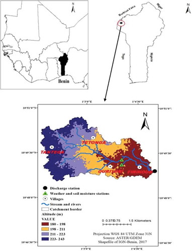
This study was carried out in the Ouriyori catchment (Fig. 1). The research area is located in the northwest of Benin, between 10°44ʹ12ʹʹN–10°55ʹ48ʹʹN and 1°01ʹ30ʹʹW–1°14ʹ30ʹʹW. The catchment is within the Dassari basin and covers an area of 14.5 km². The Ouriyori catchment is characterized by a hillslopes (in the West) drained by a tributary of the Pendjari River. The slope across the basin is 4%. The long-term (1971–2013) average monthly rainfall from the nearest rainfall station at 15 km (Tanguieta) was about 87 mm with two seasons: a rainy season, from May to mid-October, during which the maximum precipitation is reached in the months of August and September, and a dry season from November to April. The long-term temperature (1952–2010) of the nearest weather station located at 50 km (Natitingou) shows a daily range of between 15 and 39°C (Chabi 2016). The catchment is mainly dominated by croplands and fallow lands. The main soil types in the study area are tropical ferruginous soils that are relatively indurate and leached, hydromorphic soil and tropical ferruginous soils with a dominant presence of Dystric Plinthosol. There is a lot of variation in the texture and structure of the soils. The texture of the soil is mostly sandy loam characterized by a lot of gravel. Based on the census data of the Institut National de la Statistique et de l’Analyse Economique (INSAE), the Benin population growth rate was around 2.54% per year and the population density ranged from 11 to 49 inhabitants per km² during the period 2002–2013 (INSAE 2015).

Figure 1. Location of the study area

2.2 Modelling approach

2.2.1 Applied hydrological models

In this study, the WaSiM and SWAT models were applied. A brief description of the main processes used in both models is presented in Table 2. More details of the WaSiM model structure and various processes involved are provided in the WaSiM model description manual (Schulla 2015) and several early papers (e.g. Sintondji 2005, Hirekhan et al. 2007, Fasinmirin et al. 2012, Kasei 2009, Jung et al. 2012). Also, details on the SWAT model are provided in the SWAT description manual (Arnold et al. 1998) and extensively presented in previous studies (e.g. Obuobie and Diekkrüger 2008, McCartney et al. 2012, Kankam-Yeboah et al. 2013). The SWAT model is suitable for evaluating the effects of land management practices on water resources in both large and small river basins (Sudjarit 2015, Me et al. 2015).

Table 2. Different components of the models (adapted from Cornelissen et al. 2013)

	SWAT 2012	WaSiM
Soil module	Soil is divided into root and unsaturated zones	Richards’ equation
Percolation	Storage routing; travel time, up and downward flow	Function based on soil saturation and saturated conductivity
Infiltration	SCS CN procedure (1972)	Minimum of the fillable porosity and rainfall intensity
Overland flow	SCS CN procedure (1972)	Horton overland flow
Interflow	Kinematic storage model	Storage approach; comparing maximum and actual rate
Interception	Storage approach; function of LAI	Storage approach; function of LAI
Baseflow	Linear storage approach	Linear storage approach
Actual evapotranspiration	Calculated separately for evaporation (soil depth, water content) and transpiration (PET, LAI)	Separate calculation of evaporation from vegetated soils considering all soil layers and from bare soil for the first soil layer; both reduced by soil moisture content of first soil layer
Potential evapotranspiration	Priestley-Taylor, Penman-Monteith or Hargreaves	Penman-Monteith (Monteith 1975)
Routing	Lane’s Method, Continuity equation using Manning’s equation	Kinematic wave approach considering retention and translation
Spatial resolution	HRU (Hydrological Response Unit) based	Grid-based spatial discretization
Temporal resolution	Daily	Daily
Input data	DEM, Land use map and properties, soil map and properties, climate variables (rainfall, temperature, wind speed, relative humidity, solar radiation,)	DEM, land-use map and properties, soil map and properties, climate variables (rainfall, temperature, wind speed, relative humidity, solar radiation)

2.2.1.1 WaSiM

The Water flow and balance Simulation Model (WaSiM) is a deterministic, spatially distributed and physically based model for the simulation of the water cycle above and below the land surface (Schulla 2014). The hydrological processes simulated by the model include unsaturated flow, saturated flow, solute and sediment transport, surface energy balances and streamflow generation and routing. It also captures spatial variability of the catchment characteristics using spatially distributed data or boundary conditions such as vegetation, land use and soil properties, rainfall, topography, and climate among others (Schulla 2014). The model can be run in various spatial resolution (metre to kilometre grid up to 5 km) and temporal resolution (minutes to days) depending on time resolution, the catchment size, the meteorological data and the available computing power (e.g. Kasei 2009, Fasinmirin et al. 2012, Yira 2016).

2.2.1.2 SWAT

The Soil Water Assessment Tool (SWAT) is a semi-distributed model. The model delineates the catchment and its sub-basins based on a digital elevation model (DEM). The model was developed by the US Department of Agriculture - Agricultural Research Service (USDA - ARS). Water balance is computed based on meteorological, soil, and land-use data (Arnold et al. 1998, Bansode and Patil 2016, Ayele 2017). SWAT can be used to evaluate the impact of land management on water, sediment yield, and agricultural chemical transportation in large or complex catchments for various periods of time. For pre- and post-processing purposes, the model applies its continuous long-term simulations of hydro-climatic variables (Sudjarit 2015) to give significant insights into the water balance, sediments, and pollutant transfer (Bossa 2012).

2.2.2 Applied dataset

The data used for this study are summarized in Table 3. The DEM was extracted from the Advanced Spaceborne Thermal Emission and Reflection Radiometer Global Digital Elevation Model (ASTER GDEM) at the US Geological Service (USGS) website. Daily meteorological and hydrological observed data within the catchment were collected from the Benin Meteorological Directorate (Benin Meteo) and from WASCAL Data portal (wascal-dataportal.org/). Other rainfall stations close to the study area were also used. Meteorological data gaps for a given station of the catchment were filled using data of the nearest stations (Natitingou and Tanguieta). The soil map of the Ouriyouri catchment was produced based on field surveys and following the Soil and TERrain (SOTER) approach within the frame of the WASCAL project-2013. Soil properties were mainly obtained from field survey and laboratory works. The van Genuchten parameters were used to derive the soil water retention function using the pedotransfer functions (PTF) after van Genuchten (1980). The land-use maps used for the study were obtained from WASCAL data portal (Forkour 2014). Other land-use properties such as leaf area index (LAI), albedo, interception factor, root depth, etc., were derived from previous works carried out in neighbouring catchments (Kasei 2009, Bossa and Diekkrüger 2012, Cornelissen et al. 2013, Yira et al. 2016) and from the general literature. Soil moisture data were obtained from the WASCAL data portal (at the soil moisture station in the catchment). Due to dysfunction of the equipment, soil moisture data were collected only during the year 2016 under fallow and cropland.

Table 3. Summary of the data collected and used in this study

Data	Properties of the data	Parameters	Sources
DEM	30 m x 30 m	Slope, aspect, channel, curvature, sub-basin, etc	ASTER GDEM
Climate	8 weather stations, 1 synoptic station	Daily rainfall, temperature, wind speed, relative humidity, solar radiation	https://wascal-dataportal.org/geonetwork/apps/search/ and field data
Soil	1:200 000	Soil physical and chemical properties; van Genuchten parameters, Ks, θs, θres, BD etc.	https://wascal-dataportal.org/geonetwork/apps/search/ and field works
Land use	5 to 200 m	Land use classes, root depth, leaf area index, albedo, interception factor, etc.	Landsat images 2012 (Kasei 2009, Forkuor et al. 2012, Cornelissen et al. 2013, Yira et al. 2016), field works
Soil moisture	Daily (2016)	Field and fallow	https://wascal-dataportal.org/geonetwork/apps/search/ and field work
Discharge	Daily (2014–2017)	Discharge	https://wascal-dataportal.org/geonetwork/apps/search/ and field work

2.2.3 Model calibration and validation

The SWAT and the WaSiM models were run at a daily time step using the same climate, land use, soil and discharge dataset. Both models were calibrated for the period 2014–2015 and validated for the period 2016–2017. The choice of calibration and validation periods in this study was based on the length of available hydroclimatic data. In addition, 3 years of data were considered as warm-up period for the models.

A number of parameters (nine in this study) need to be calibrated to set up WaSiM (Shulla 2014). These parameters include the saturated hydraulic conductivity with soil depth (K_rec), the interflow drainage density (dr), the coefficient for surface flow (kd), the interflow storage coefficient (ki), the soil surface resistance for evaporation (rs_evaporation), the interception surface resistance (rs_interception), the baseflow coefficient (K) in the equation $q_b=Q_o.\mathrm{e}\mathrm{x}{\mathrm{p}}^{\left(-k/z\right)}$ with $Q_o$ the baseflow coefficient, the saturated hydraulic conductivity (K_s) and the soil moisture parameters. For the SWAT model, a semi-automatic and uncertainty analysis was performed applying the SUFI-2 procedure (Sequential Uncertainty Fitting version 2, SWAT-CUP interface (Abbaspour 2008)), involving 13 parameters. The SUFI-2 algorithm searches for the best-fitted parameter values by predicting uncertainties related to model structure, input and output data, model parameters (Abbaspour et al. 2004, 2007). Following the SUFI-2 approach and according to Abbaspour (2011) as well as Narsimlu et al. (2015), all the uncertainties are expressed by coefficients such as the p-factor (percentage of measured data bracketed by the 95% prediction uncertainty) and r-factor (ratio between the average thickness of the 95PPU band and the standard deviation of the measured data). The p-factor ranges between 0 and 1. The close the r-factor is to 1, the better is the model performance. Thus, these coefficients show the performance of the model during the simulation process (Taghvaye et al. 2016).

To evaluate the goodness of fit between the simulated and observed variables for both models, four evaluation criteria were applied: (i) the coefficient of determination (R²), (ii) the Nash-Sutcliffe efficiency coefficient (NSE) (Nash and Sutcliffe 1970), (iii) the Kling-Gupta efficiency (KGE) (Kling et al. 2012), and (iv) the percent bias (PBIAS) (Gupta et al. 1999). Simulations were deemed satisfactory when NSE ≥ 0.5; KGE ≥ 0.5; R² ≥ 0.5 following Moriasi et al. (2007) and absPBIAS ≤ 25%.

2.3 Assessment of hydrological ecosystem services

The Organization for Economic Co-operation and Development (OECD) and European Commission (EC) (2013) showed that the service flow of a catchment’s ecosystems can be classified into the capacity of the catchment to provide the services and the flow of hydrological services itself. Service flow is the contribution of an ecosystem, in space and time, to a utility function or a production function for human’s benefit. At the same time, the service capacity refers to the ecosystem condition and extent at a point in time and the resulting potential to provide service flows (EC et al. 2013).

The calibrated and validated model results are analysed along with the ecosystem accounting framework to quantify the flows and the capacities of hydrological ecosystem services using additional information such as demographical data. Crop water supply, household water supply (surface and groundwater supply) were the hydrological ecosystem services evaluated in this study. The interest of this study for these particular HES is justified by commonly critical issues for rural communities in terms of food and water security. Moreover, for both drinking and other household activities, groundwater is the main water source in the study area. The hydrological ecosystem services of interest and associated service flow and service capacity indicators are presented in Table 4.

Table 4. Selected hydrological ecosystem services and associated service flow and service capacity indicators (GP is growing period) (following: EC, OECD 2013, Duku et al. 2015)

Hydrological ecosystem services		Service flow indicator	Service capacity indicator
Crop water supply		Total number of days during the growing period in which there was no water stress (d GP^−1)	Total number of days in a year when the sum of actual evapotranspiration and the amount of residual moisture added to the soil profile equaled or exceeded 75% of the potential evapotranspiration (d year^−1)
Household water supply	Groundwater supply	Amount of groundwater extracted (mm year^−1)	Groundwater recharge (mm year^−1)
	Surface water supply	Amount of surface water extracted (mm year^−1)	Water yield (mm year^−1)

2.4 Crop water supply

Crop water supply refers to the provision of plant available water during ecohydrological processes in rainfed agriculture systems (IWMI 2007, Zang et al. 2012). In a rainfed agricultural system, crop water stress is considerably reduced by soil moisture supply. In this study, crop water supply was restricted to upland crop (maize). Service flow of crop water is quantified as the total number of days during a growing period in which there was no water stress. In other words, it represents the days when the total plant water uptake was sufficient to meet plant water demand (Duku et al. 2015). As maize remains the most cultivated crop in the study area and represents more than 60% of agricultural areas (Forkour 2014), for the sake of simplicity, only maize cultivation is considered in the crop water supply analysis. The growing period (GP) which refers to the time period between crop establishment and harvesting was 103 days for maize (Duku et al. 2015). The establishment of maize is in the month of June. Equation 1(1) $S_f=N\left(d_1,d_2,d_3\dots ,d_n|W_{\mathrm{s}\mathrm{t}\mathrm{r}\mathrm{s}}\le 0.25\right)$(1) (modified, after Duku et al. 2015) is used to compute the service flow.

(1) $S_f=N\left(d_1,d_2,d_3\dots ,d_n|W_{\mathrm{s}\mathrm{t}\mathrm{r}\mathrm{s}}\le 0.25\right)$(1)

where S_f is the service flow (d GP⁻¹), N the number of days d₁ to d_n and W_strs is the daily water stress.

This approach was based on commonly applied FAO methods for the determination of the length of growing periods in rainfed agriculture, gives an indication regarding the potential total number of days when there will be no crop water stress according to the crop type (FAO 1978, 1983). This is therefore relevant for the crop and water management.

The daily water stress is calculated by the model following equation (2)(2) $W_{\mathrm{s}\mathrm{t}\mathrm{r}\mathrm{s}}=1-\left(\frac{T_{\mathrm{a}\mathrm{c}\mathrm{t}}}{T_{\mathrm{m}\mathrm{a}\mathrm{x}}}\right)$(2) :

(2) $W_{\mathrm{s}\mathrm{t}\mathrm{r}\mathrm{s}}=1-\left(\frac{T_{\mathrm{a}\mathrm{c}\mathrm{t}}}{T_{\mathrm{m}\mathrm{a}\mathrm{x}}}\right)$(2)

where T_act is plant water uptake or actual transpiration (mm), and T_max is maximum plant water demand or maximum transpiration (mm).

In this study, soil moisture supply is based on simulated soil moisture dynamics. This approach is used because precipitation attributes such as quantity, location, timing and intensity are slightly impacted by terrestrial ecosystem attributes at local scale (Duku et al. 2015).

The service capacity of crop water supply is expressed by as follows:

(3) $S_C=N\left(d_{1,\hspace{0.17em}}\hspace{0.17em}{d}_{2\hspace{0.17em}},\dots .,d_n|W_{\mathrm{p}\mathrm{s}\mathrm{t}\mathrm{r}\mathrm{s}}\le 0.25\right)$(3)

where S_c is the service capacity (d year⁻¹); N the number of days d₁ to d_n in a year when potentially there will be no water stress and W_pstrs is the potential daily water stress. W_pstrs is derived from the water balance and expressed as follows:

(4) $W_{\mathrm{p}\mathrm{s}\mathrm{t}\mathrm{r}\mathrm{s}}=1-\left[\left(\mathrm{\Delta }\mathrm{S}\mathrm{W}+\mathrm{E}{\mathrm{T}}_a\right)/\mathrm{E}{\mathrm{T}}_P\right]\mathrm{i}\mathrm{f}\mathrm{\Delta }\mathrm{S}\mathrm{W}>0$(4)

2.5 Household water supply

In this study, the household water supply is the amount of water extracted for household consumption for drinking and non-drinking (OECD 2013). The population in our research area obtained about 80% of their drinking water from groundwater (INSAE 2015). Water consumption per day per person was estimated to 30 L (UNDP 2017). These data considered both drinking and non-drinking water consumption of the households. The population of the catchment was about 1018 with 143 households in 2013 (INSAE 2015). The water consumption per capita is kept constant and a population rate of 3.06% per year (INSAE 2015) was used to estimate the population growth. Groundwater recharge, which is the amount of water entering the aquifer during a specific period of time, is quantified as the ecosystem capacity for groundwater extraction. Meanwhile, the water yield, which is the amount of water contributing to the river network during a specific period of time, is quantified as the ecosystem capacity to support surface water extraction (Arnold et al. 1998).

3 Results

3.1 Model calibration and validation

Based on literature review, in the calibration procedure, nine parameters were optimized for the WaSiM model against 13 parameters for SWAT. The Soil Conservation Service Curve Number (CN2), the soil evaporation compensation factor (ESCO), the threshold water level in a shallow aquifer for capillary rise (REVAPMN), the effective channel hydraulic conductivity (Ch_K2), and the soil available water storage capacity (SOL_AWC) were found to be the best-fitted parameters for the SWAT model following the SUFI-2 procedure. As for the WaSiM model, the interflow drainage density (dr), the coefficient for surface flow (kd), the interflow storage coefficient (ki), the baseflow coefficient (K) and the baseflow coefficient (Qo) were the best following a one-factor-at-a-time sensitivity analysis. The calibrated values for both models are shown in Table 5. The quantifiers v_, r_ and a_ stand, respectively, for the substitution of a parameter by a value from the given range mean values, relative change and absolute change. ALPHA_BF, GW_DELAY, GWQMN, SURLAG, RCHRG_DP, SOL_K, GW_REVAP and CH_N2 are, respectively, the baseflow alpha factor characterising the groundwater recession curve, the time required for water leaving the bottom of the root zone to reach the shallow aquifer, the soil available water storage capacity (SOL_AWC), the minimum water level for baseflow generation, the surface runoff lag coefficient, the deep aquifer percolation coefficient, the saturated hydraulic conductivity, the groundwater “revaporation” coefficient and Manning’s n value for the main channel.

Table 5. Calibrated and fitted parameter values in WaSiM and SWAT simulation

Parameter name	Initial range	Calibrated range	Fitted values	Units
WaSiM
kd	1–110	-	40	-
ki	1–110	-	50	-
dr	10–100	-	22.4	-
K	0.1–2.5	-	0.5	m
Qo	0.1–2.5	-	0.1	mm d^−1
SWAT
a_CN2.mgt	[– 10;55]	[34.57;52.06]	38.51	-
v_ALPHA_BF.gw	[0.05;0.7]	[0.40;0.64]	0.46	d
v_GW_DELAY.gw	[0.01;20]	[2.08;3.58]	2.22	d
v_GWQMN.gw	[10;40]	[19.74;24.32]	25.57	mm
v_ESCO.hru	[0;0.15]	[0.78;1.34]	1.14	-
v_SURLAG.bsn	[0.1;0.5]	[0.49;0.64]	0.58	-
v_RCHRG_DP.gw	[0;0.01]	[0;0.01]	0.01	-
r_SOL_K.sol	[0.1;2]	[0.43;1.29]	0.83	mm h^−1
v_REVAPMN.gw	[20;35]	[35.64;38.83]	34.41	mm
v_GW_REVAP.gw	[0.5;2]	[1.11;1.76]	1.69	-
v_CH_K2.rte	[1;15]	[10.09;13.56]	13.84	-
r_SOL_AWC.sol	[0;0.15]	[0.03;0.05]	0.01	mm mm^−1 (H2O/soil)
v_CH_N2.rte	[0;0.5]	[0.23;0.30]	0.28	-

3.2 Water balance components

Water balance components for each model used in the study (Table 6) were compared with the simulation results of other studies conducted in neighbouring basins. For both models, the performance statistics (R², NSE, KGE and absPBIAS) revealed good simulations, ascertaining the ability of the models to capture the discharge occurring at the catchment outlet.

Table 6. Catchment water balance for calibration and validation periods with corresponding performance statistics (percentage in parentheses)

Hydrological models	Calibration (2014–2015)		Validation (2016–2017)
	WaSiM	SWAT	WaSiM	SWAT
Rainfall (mm)	941.8	915.2	883.2	698
Etp (mm)	2186.8	1907.6	2238.6	1748.3
Eta (mm)	771.1	609.1	821.6	548.2
Total discharge (mm)	187.9	246.6	136.4	128.6
Surface runoff (mm)	122.5 (65.2%)	125.5 (50.9%)	97.1 (71.2%)	76.2 (59.3%)
Baseflow (mm)	0.5 (0.0%)	100.2 (40.6%)	0.4 (0.3%)	37 (28.8%)
Interflow (mm)	64.9 (35.6%)	20.8 (8.5%)	38.8 (28.5%)	15.4 (11.9%)
R^2	0.7	0.8	0.7	0.8
NSE	0.7	0.8	0.7	0.8
KGE	0.7	0.9	0.6	0.8
absPBIAS (%)	24.7	3.6	22.8	16.2

SWAT generally shows higher performance compared to WaSiM, taking advantage of the SUFI-2 approach (Arnold et al. 1998) used for SWAT calibration against the one-factor-at-a-time approach used for WaSiM. Consistently to that, surface runoff and baseflow are found to be the major discharge components simulated by the SWAT model, while WaSiM rather indicated surface runoff and interflow as the major simulated discharge components (Table 6). These results of SWAT are similar to the findings of Bossa and Diekkrüger (2012) in the Ouéme basin and are also in line with the results obtained in the Terou basin (Cornelissen et al. 2013). Meanwhile, the results achieved with the WaSiM model corroborate the findings of Yira (2016) and Kasei (2009) in the Dano catchment and the Volta basin, respectively (Table 7). It is also reported, following SWAT applications, that baseflow was the most predominant streamflow process in the White Volta basin (Oboubie 2008), in the Okpara basin (Sintondji et al. 2013) and the Couffo basin (Sintondji et al. 2017). Besides differences in model parameterizations, the rainfall interpolation techniques (the closest of the centroid sub-basin for SWAT and the inverse distance weighting method for WaSiM) of each model may explain the differences in simulated discharge components.

Table 7. Water balance components of neighbouring catchments

Authors	Model	Study area (catchment)	Streamflow components (%)
			Surface runoff	Baseflow	Interflow
Kasei 2009	WaSiM	Volta basin (West Africa)	23–30	10–12	60–69
Yira 2016		Dano (Burkina-Faso)	38–50	3–11	45–56
Cornelissen et al. 2013		Terou (Benin)	50	24–25	25–26
Badou 2016		Benin portion of the Niger River basin (Benin)	31–48	37–59	7–15
Bossa and Diekkrüger 2012	SWAT	Ouémé basin (Benin)	34–54	46–66	-
Cornelissen et al. 2013		Terou (Benin)	43–45	55–57	0
Badou 2016		Benin portion of the Niger River basin (Benin)	56–96	2–41	0–42
Oboubie, 2008		White Volta basin (West Africa)	32–35	65–67	0
Sintondji et al. 2013		Okpara (Benin)	39–44	55–60	1

3.3 Simulation of streamflow

The calibration and validation can be judged as good for both models based on the statistical coefficients. However, for SWAT, the p-factor failed to achieve a threshold of 0.70 for streamflow for both the calibration and validation phases. The percentage of the prediction uncertainty (95PPU) enveloped only 31% of the estimated flow for the simulations. This percentage is partly due to the length of available climatic dataset. Regarding the r-factor, a coefficient of 0.14 was obtained for the calibration step and 0.20 for the validation step. As for the achieved p-factor, it only bracketed 25% to 55% of the observed discharge.

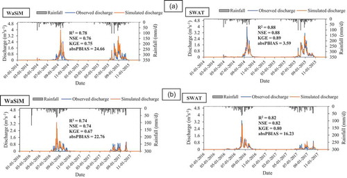
High correlations were shown between the observed and simulated daily discharge (Fig. 2), indicating good performance for both models. The difference between the observed and simulated mean discharge for the calibration period was estimated as 0.006 and 0.038 m³ s⁻¹ for the SWAT and WaSiM models, respectively, against 0.011 and 0.014 m³ s⁻¹ for the validation. In general, one can see that SWAT slightly underestimated the discharge against an overestimation for the WaSiM model over both the calibration and validation periods (Fig. 2).

Figure 2. Observed and simulated discharge for (a) during the calibration period and (b) the validation period for both WaSiM and SWAT models. R², NSE and KGE refer to Pearson product-moment-correlation-coefficient, Nash-Sutcliffe efficiency and Kling-Gupta efficiency, respectively, and absPBIAS refers to the absolute value of PBIAS

3.4 Soil moisture

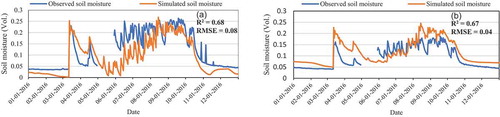
Simulated and observed soil moisture with WaSiM were compared at two different soil depths (6 and 24 cm), which encompasses the top 30 cm of the soil profile in the year 2016. Since soil water retention parameters (soil permeability, bulk density, available water content of soil, hydraulic conductivity, field capacity and wilting point) were derived from laboratory analysis, they were not optimized for the calibration. For the SWAT model, soil moisture was extracted at the hydrologic response unit level from the final model output. Thus, the simulated soil moisture content was converted into relative soil moisture (percentage) and later into total soil moisture for each soil layer. The results indicate good performance for WaSiM: the model is able to simulate the dynamic of soil moisture across two different layers. In the first layer (6 cm), simulated and observed soil moisture shows good agreement proving that the model was able to capture the dynamic of soil moisture (Fig. 3(a)). An under-estimation (up to 0.05 vol.) of the soil moisture is observed for the middle of the year (June–August). In a similar way, the comparison of simulated and observed soil moisture in the second layer (24 cm) revealed good agreement as well (Fig. 3(b)). However, an overestimation (up to 0.05 vol.) may be observed, particularly at the beginning and end of the year (September–December). Given that SWAT simulates soil moisture only for the whole soil profile and not for individual soil layers, it has not been considered for soil moisture simulation. One has to recall that, for this study, observed soil moisture data were available for the upper two soil layers.

Figure 3. Comparison of simulated and observed soil moisture at a daily time step: (a) at the first horizon at 6 cm depth, and (b) of the second horizon at 24 cm depth. R²: Pearson product-moment correlation-coefficient; RMSE: refers to root mean square error

3.5 Hydrological ecosystem services

Table 8 shows service flow and service capacity for both models. For the simulated 4 years, the mean annual values of crop water supply service capacity range from 42 to 49 d year⁻¹ with an average of 45 d year⁻¹ for the catchment and a standard deviation of 3 d year⁻¹ for the SWAT model, whereas, for the WaSiM model, the mean annual values of the same service capacity ranges from 56 to 97 d year⁻¹ with an average of 85 d year⁻¹ and a standard deviation of 19 d year⁻¹. Regarding the mean seasonal values of the service flow, it ranges according to SWAT simulations, from 27 to 45 d GP⁻¹ with a mean of 42 d GP⁻¹ and a standard deviation of 13 d GP⁻¹. In a similar way for the WaSiM model, the mean seasonal values of the service flow range from 23 to 68 d GP⁻¹ with a catchment mean of 51 d GP⁻¹ and a standard deviation of 19 d GP⁻¹. Therefore, compared to the maize growing period, i.e. 103 days (Duku et al. 2015), the crop water supply service capacity, irrespective of the hydrological model, indicates that the crop undergoes water stress for at least 25 days per growing cycle. This implies that even if other crop growth factors (soil fertility, nutrients, temperature, soil type) are optimized, crop yield is likely to remain low due to water stress.

Table 8. Hydrological ecosystem services and associated service flow and service capacity indicators with WaSiM and SWAT models

Hydrological ecosystem service		Service flow indicator				Service capacity indicator
		2014	2015	2016	2017	2014	2015	2016	2017
WaSiM
Annual rainfall (mm)		880.56	1002.96	983.02	783.39	880.56	1002.96	983.02	783.39
Crop water supply		(d GP^−1)				(d year^−1)
		23	54	57	68	56	92	97	93
Household water supply	Groundwater supply	(mm year^−1)
		64.1	64.8	65	69.1	116.5	133	112.4	107
	Surface water supply	16	16.5	17	17.5	147.9	228	158.9	113.8
SWAT
Annual rainfall (mm)		853.8	976.5	839.04	557	853.8	976.5	839.04	557
Crop water supply		(d GP^−1)				(d year^−1)
		27	45	40	37	43	45	49	42
Household water supply	Groundwater supply	(mm year^−1)
		64	64.8	65	69.1	107.9	183.3	101.4	65.8
	Surface water supply	16.1	16.5	17	17.5	179.5	326.1	185.5	80.8

The mean annual values of service flow and service capacity of groundwater supply and surface water supply are also shown in Table 8. As may be seen, there is an increasing trend in service flow of crop water supply. The service flow (groundwater extraction) within the catchment is significantly higher than the service flow of surface water supply (surface water extraction). This situation, as already stated, may be due to the fact that groundwater is the major water source (drinking and non-drinking) for household consumption in the catchment. While surface water is only available for a couple of months, groundwater is potentially available throughout the year. According to the WaSiM model, the service capacity of groundwater supply increased from 116.5 to 133 mm (from 2014 to 2015), and decreased thereafter from 112.4 to 107 mm (from 2016 to 2017). With the SWAT model, for the same periods, the capacity of groundwater supply followed a similar trend, increasing from 107.9 to 183.3 mm (from 2014 to 2015), and decreasing from 101.4 to 65.8 mm (from 2016 to 2017). Thus, the groundwater availability was higher for the years 2014 and 2015, compared to the years 2016 and 2017, as a consequence of inter-annual rainfall variability.

With regard to the surface water supply, the service flow ranges from 16.05 to 17.53 mm year⁻¹. Meanwhile, the service capacity decreased, from 228.01 to 113.81 mm year⁻¹ with WaSiM and 326.14 to 80.79 mm year⁻¹ with SWAT between 2015 and 2017. The annual surface water capacity is high with SWAT compared to WaSiM. In addition, the catchment shows a high service capacity of surface water supply consistently with the simulated water yield. This situation occurred frequently in savanna and shrubland where areas are hydrologically sensitive (Agnew 2006, Duku et al. 2015).

A weak capacity of ecosystems to sustain human welfare over time is a measure of ecosystem degradation (OCED 2013). A high swing is observed in the crop water service flow with WaSiM, whereas a mixed direction is observed with SWAT. High values of crop water supply capacity were observed for both models with a lower value after 2016. For groundwater, a lower service capacity was observed for both models after 2015. The same situation was observed for surface water supply capacity.

4 Discussion

For both WaSiM and SWAT, the daily simulations responded well to rainfall events. In addition, the overall performance – in terms of R², NSE, KGE and absPBIAS – can be judged as good, especially considering the limited data conditions of the study (Chaibou Begou et al. 2016, Yira 2016). On a daily basis, R² was 0.7 and 0.8, respectively, for WaSiM and SWAT in the calibration period and 0.7 and 0.8 in the validation period. NSE was 0.7 for WaSiM and 0.8 for SWAT for the calibration and validation periods, while KGE varied between 0.6 and 0.7 for WaSiM and 0.8 and 0.9 for SWAT (calibration and validation steps, respectively). The absPBIAS was lower than 25% for both models.

These results are comparable to those of Badou (2016), Obuobie and Diekkrüger (2008), Yira (2016) and Bossa and Diekkrüger (2012) in nearby basins. Although observations are limited for discharge components, compared to reference studies in the region, the water balance appears relatively well simulated. However, differences in discharge components can be noted between the two models. This difference may be related to the model parameters’ optimization during the simulation. The uncertainty analysis showed a relatively low satisfaction as the 95PPU only bracketed 31% of the observed discharge. These results are comparable to the findings of Osei et al. (2018) who achieved a 95PPU that bracketed only 45% of the streamflow data. With the exception of the p-factor, the performance indicators (R², NSE, KGE and absPBIAS) showed satisfactory performance of the models.

The empirical distinction and separate characterization of service capacity and service flow are essential in understanding the dynamics of service provision and in planning and devising sustainable management options (Duku et al. 2015). One notices that service capacity is higher than the service flow, meaning an under-utilization of HES in the catchment a priori. This implies, among others, that the catchment can potentially supply more water needed for maize growth and other related crops having similar water requirements assuming optimal water management conditions. It was shown by Shaxson and Barber (2003) that crop water supply is one of the main limitations for crop production in rainfed agriculture systems and thereby the major factor causing low crop yield in semi-arid areas.

The water service flow is lower than the service capacity of the catchment for household water supplies. As groundwater remains the major source of water for consumption by households, the service flow in terms of groundwater extraction was significantly higher than the service flow of surface water supply. It should be noted that the service capacity of groundwater supply is lower than that of the surface water supply. Despite a high service capacity, service flow for surface water supply is only possible for a limited period (July to December) before rivers dry up. This highlights the need for storage and management of surface water to improve water availability in the catchment.

Consistently with the annual rainfall, the service capacity for groundwater supply exhibited high values from 2014 to 2015 and low values thereafter. Notwithstanding this variability due to the inter-annual rainfall of the catchment, the catchment is capable of supplying groundwater services. This situation is comparable to the results achieved in the Ouémé catchment (which is close to the Ouriyori), where service capacity was found to be high too (Duku et al. 2015).

5 Conclusion

The SWAT and WaSiM models were calibrated and validated in the Ouriyori catchment (14.5 km²) using, amongst others, daily observed climate and discharge data. Both models were able to reproduce adequately the daily discharge at the catchment outlet, although the SWAT simulations achieved higher performance. The study confirms the ability of both models to reproduce hydrological conditions of small catchments of some square kilometers. It is worth mentioning that Wallace et al. (2018) achieved satisfactory simulation results with little effect of catchment size on simulated flows, applying the SWAT model for catchments ranging from 20 to 680 km².

The SWAT and WaSiM models have successfully supported the computation of reliable and meaningful HES indicators through simulated data (plant growing days with water stress, actual evapotranspiration, residual soil moisture, potential evapotranspiration, groundwater recharge, water yield, etc.). Thus, HES capacity and flow, which are the key components that need to be measured to capture the full dynamics of ecosystem service provision, were estimated and showed that the service capacities for both crop and household water supply are higher than their service flow. Furthermore, a high service capacity of surface water compared to that of the groundwater was shown, while the service capacity of crop water supply was revealed higher than its service flow. These significant results suggest that strategic sustainable actions may be taken to increase water and food security and subsequently improve resilience and adaptation to climate variability. Amongst other actions, water retention systems can be implemented in such a way as to extend the availability period of surface water and groundwater supply capacity (and use). In addition, rice production and off-season farming may be implemented, taking advantage of the water availability, despite the prevailing inter-annual rainfall variability. Actions could include the implementation of soil and water conservation systems to considerably increase the groundwater recharge (capacity) through the recharge of aquifers. This study showed that hydrological modelling can lead to reliable hydrological ecosystem service assessment with relevant and suitable information for sustainable management of catchment ecosystem services and decision-making.

Acknowledgements

The authors would like to thank Prof. Ilyas Masih and Mrs Jeewa T. Arachchillage from IHE Delft Institute for Water Education (The Netherlands) for technical assistance. They are very grateful to Dr Stefan Liersch, who provided insightful comments that helped to improve the manuscript. The authors are particularly grateful to Professor Bernd Diekkrüger, Mr Gero Steup and Dr Felix Op de Hipt for designing and implementing the data collection and processing systems. Finally, they are thankful to the German Federal Ministry of Education and Research (BMBF) (Grant No. 01LG1202E) for the financial support provided under the auspices of the West African Science Service Centre for Climate Change and Adapted Land Use (WASCAL).

Disclosure statement

No potential conflict of interest was reported by the authors.

Additional information

Funding

This work was supported by the West African Science Service Centre on Climate Change and Adapted Land Use programme.

References

- Abbaspour, K.C., 2008. SWAT calibrating and uncertainty programs. A user manual. Zurich, Switzerland: Eawag, Swiss Federal Institute of Aquatic Science and Technology.
- Abbaspour, K.C., 2011. SWAT-CUP4: SWAT calibration and uncertainty programs – A user manual. Zurich, Switzerland: Eawag, Swiss Federal Institute of Aquatic Science and Technology.
- Abbaspour, K.C., Johnson, C., and Van Genuchten, M.T., 2004. Estimating uncertain flow and transport parameters using a sequential uncertainty fitting procedure. Vadose Zone Journal, 3, 1340–1352. doi:10.2136/vzj2004.1340
- Abbaspour, K.C., Vejdani, M., and Haghighat, S., 2007. SWAT-CUP calibration and uncertainty programs for SWAT. In: Proc. Intl. Congress on Modelling and Simulation (MODSIM’2007), Melbourne, Australia, 1603–1609.
- Agnew, L.J., 2006. Identifying hydrologically sensitive areas: bridging the gap between science and application. Journal of Environmental Management, 78, 63–76. doi:10.1016/j.jenvman.2005.04.021.
- Aich, V., et al., 2015. Climate or land use? Attribution of changes in river flooding in the Sahel Zone. Water, 7 (6), 2796–2820. doi:10.3390/w7062796
- Alam, M.J., Meah, M.A., and Noor, M.S., 2011. Numerical modelling of groundwater flow and the effect of boundary condition for the hsieh aquifer. Asian Journal of Mathematics & Statistics, 4, 33–44. doi:10.3923/ajms.2011.33.44
- Arnold, J. G., Srinivasan, R., Muttiah, R. S., and Williams, J. R., 1998. Large area hydrologic modeling and assessment–Part 1: Model development. Journal of the American Water Resources Association, 34, 73–89.
- Arnold, J.G., et al., 1998. Large area hydrologic modelling and assessment part I: model development 1. JAWRA Journal of the American Water Resources Association, 34 (1), 73–89. doi:10.1111/j.1752-1688.1998.tb05961.x
- Ayele, G.T., 2017. Streamflow and sediment yield prediction for watershed prioritization in the Upper Blue Nile River Basin, Ethiopia. Water, 9, 782. doi:10.3390/w9100782
- Badou, D.F., 2016. Multi-model evaluation of blue and green water availability under climate change in Four-Non Sahelian Basins of the Niger River Basin. Thesis (PhD). University of Abomey-calavi.
- Badou, D.F., et al., 2017. Evaluation of recent hydro-climatic changes in four tributaries of the Niger River Basin (West Africa). Hydrological Sciences Journal, 62 (5), 715–728. doi:10.1080/02626667.2016.1250898
- Bansode, S. and Patil, K., 2016. Water balance assessment using Q-SWAT. Int J Eng Res, 5 (6), 2319–6890.
- Bergström, S., 1976. Development and application of a conceptual runoff model for Scandinavian catchments. No. RH07. Norrköping: Meteorol. and Hydrol. Inst.
- Bergström, S., 1992. The HBV model - its structure and applications, SMHI Hydrology, RH No.4, Norrkoping, 35.
- Beven, K., 2006. A manifesto for the equifinality thesis. Journal of Hydrology, 320 (1–2), 18–36. doi:10.1016/j.jhydrol.2005.07.007
- Biazin, B., et al., 2012. Rainwater harvesting and management in rainfed agricultural systems in sub-Saharan Africa–a review. Physics and Chemistry of the Earth, Parts A/B/C, 47, 139–151. doi:10.1016/j.pce.2011.08.015
- Boorman, D.B., and Sefton, C.E.M., 1997. Recognising the uncertainty in the quantification of the effects of climate change on hydrological response. Climatic Change, 35(4), 415–434.
- Bormann, H., 2005. Evaluation of hydrological models for scenario analyses: signal-to-noise-ratio between scenario effects and model uncertainty. Advances in Geosciences, 5, 43–48. doi:10.5194/adgeo-5-43-2005
- Bossa, A.Y., 2012. Multi-scale modelling of sediment and nutrient flow dynamics in the Ouémé catchment (Benin) – towards an assessment of global change effects on soil degradation and water quality. Thesis (PhD). Rheinischen Friedrich-Wilhelms-Universität Bonn.
- Bossa, A.Y. and Diekkrüger, B., 2012. Estimating scale effects of catchment properties on modelling soil and water degradation in Benin (West Africa). International Congress on Environmental Modelling and Software, 185. https://scholarsarchive.byu.edu/iemssconference/2012/Stream-B/185
- Bossa, A.Y., Diekkrüger, B., and Agbossou, E.K., 2014. Scenario-based impacts of land use and climate change on land and water degradation from the meso to regional scale. Water, 6 (10), 3152–3181. doi:10.3390/w6103152.
- Breuer, L., et al., 2009. Assessing the impact of land use change on hydrology by ensemble modelling (LUCHEM). I: model intercomparison with current land use. Advances in water resources, 32 (2), 129–146.
- Chabi, A., 2016. Land-use change modelling, scenarios development and Impacts assessment on CO2 and N2O emissions from vegetation degradation in the Dassari basin, Benin. Thesis (PhD). Ghana: Kwame Nkrumah University of Science and Technology
- Chaibou Begou, J., et al., 2016. Multi-site validation of the SWAT model on the Bani catchment: model performance and predictive uncertainty. Water, 8 (5), 178. doi:10.3390/w8050178
- Chan, K.M., et al., 2006. Conservation planning for ecosystem services. PLoS Biology, 4, 11. doi:10.1371/journal.pbio.0040379
- Cornelissen, T., Diekkrüger, B., and Giertz, S., 2013. A comparison of hydrological models for assessing the impact of land use and climate change on discharge in a tropical catchment. Journal of Hydrology, 498, 221–236. doi:10.1016/j.jhydrol.2013.06.016
- Duan, Q., et al., 2007. Multi-model ensemble hydrologic prediction using Bayesian model averaging. Advances in Water Resources, 30 (5), 1371–1386. doi:10.1016/j.advwatres.2006.11.014
- Duku, C., et al., 2015. Towards ecosystem accounting: a comprehensive approach to modelling multiple hydrological ecosystem services. Hydrology & Earth System Sciences Discussions, 12, 3. doi:10.5194/hessd-12-3477-2015
- FAO (Food and Agriculture Organization of the United Nations), 1978. Report on the AgroEcological zones project, vol. 1. Methodology and results for Africa. Rome: UNESCO, Paris and FAO.
- FAO (Food and Agriculture Organization of the United Nations), 1983. Guidelines: land evaluation for rainfed agriculture. Food and Agriculture Organization of the United Nations. Soils Bulletin, 52. Rome: FAO.
- Fasinmirin, J.T., Olufayo, A.A., and Oguntunde, P.G., 2012. Calibration and validation of a soil water simulation model (WaSiM) for field grown Amaranthus cruentus. International Journal of Plant Production, 2 (3), 269–278. doi:10.22069/IJPP.2012.618
- Foley, A.M., 2010. Uncertainty in regional climate modelling: A review. Progress in Physical Geography: Earth and Environment, 34 (5), 647–670. doi:10.1177/0309133310375654
- Forkour, G., 2014. Agricultural land use mapping in West Africa using multi-sensor satellite imagery. Thesis (PhD). Julius-Maximilians-Universität Würzburg, Germany. http://opus.uni-wuerzburg.de/files/10868/Thesis_Gerald_Forkuor_2014.pdf.
- Forkuor, G., Landmann, T., Conrad, C. and Dech, S., 2012. Agricultural land use mapping in the sudanian savanna of West Africa: Current status and future possibilities. In 2012 IEEE International Geoscience and Remote Sensing Symposium (pp. 6293–6296). IEEE.
- Giertz, S., et al., 2010. Hydrological processes and soil degradation in Benin. In: P. Speth, M. Christoph, and B. Diekkrüger, eds. Impacts of global change on the hydrological cycle in West and Northwest Africa. Germany: Springer, Berlin, 168–197.
- Golmohammadi, G., et al., 2014. Evaluating three hydrological distributed watershed models: MIKE-SHE, APEX, SWAT. Hydrology, 1 (1), 20–39. doi:10.3390/hydrology1010020
- Gupta, H.V., Sorooshian, S., and Yapo, P.O., 1999. Status of automatic calibration for hydrologic models: comparison with multilevel expert calibration. Journal of Hydrologic Engineering, 4 (2), 135–143. doi:10.1061/(ASCE)1084-0699(1999)4:2(135)
- Haddeland, I., et al., 2011. Multimodel estimate of the global terrestrial water balance: setup and first results. Journal of Hydrometeorology, 12 (5), 869–884. doi:10.1175/2011JHM1324.1
- Hattermann, F.F., et al., 2018. Sources of uncertainty in hydrological climate impact assessment: a cross-scale study. Environmental Research Letters, 13, 015006. doi:10.1088/1748-9326/aa9938
- Hiepe, C., 2008. Soil degradation by water erosion in a sub-humid West-African catchment: a modelling approach considering land use and climate change in Benin. Thesis (PhD). Germany: Rheinischen Friedrich-Wilhelms-Universität Bonn.
- Hirekhan, M., Gupta, S.K., and Mishra, K.L., 2007. Application of WaSim to assess performance of a subsurface drainage system under semi-arid monsoon climate. Agricultural water management, 88(1–3), 224–234.
- Hollinger, F. and Staatz, J.M., 2015. Agricultural Growth in West Africa. In: Market and policy drivers. Pobrano październik: FAO, African Development Bank, ECOWAS.
- Huisman, J.A., Breuer, L., Bormann, H., Bronstert, A., Croke, B. F. W., Frede, H., Gräff, T., et al., 2009. Assessing the impact of land use change on hydrology by ensemble modeling (LUCHEM) III : Scenario analysis. Advances in Water Resources, 32, 159–170. doi:10.1016/j.advwatres.2008.06.009
- INSAE/RGPH 4, 2015. Quatrième Recensement Général de la Population et de l'Habitation (2013): Que retenir des effectifs de population en 2013? INSAE, Cotonou, Bénin, 35 p
- IWMI, 2007. Water for food, water for life: a Comprehensive Assessment of Water Management in Agriculture. International Water Management Institute. Earthscan, London, UK.
- Jiang, T., Chen, D. Y, Xu, C., Chen, X., Chen, X., and Singh, V. P., 2007. Comparison of hydrological impacts of climate change simulated by six hydrological models in the Dongjiang Basin, South China. Journal of Hydrology. 336, 316–333. doi:10.1016/j.jhydrol.2007.01.010
- Jung, G., Wagner, S., and Kunstmann, H., 2012. Joint climate-hydrology modelling: an impact study for the data-sparse environment of the Volta Basin in West Africa. Hydrology Research, 43, 231–248. doi:10.2166/nh.2012.044
- Kankam-Yeboah, K., et al., 2013. Impact of climate change on streamflow in selected river basins in Ghana. Hydrological Sciences Journal, 58 (4), 773–788. doi:10.1080/02626667.2013.782101
- Kannan, N., et al., 2007. Hydrological modelling of a small catchment using SWAT-2000–Ensuring correct flow partitioning for contaminant modelling. Journal of Hydrology, 334 (1–2), 64–72. doi:10.1016/j.jhydrol.2006.09.030
- Kasei, R.A., 2009. Modelling impacts of climate change on water resources in the Volta Basin, West Africa. Thesis (PhD). University of Bonn. http://hss.ulb.uni-bonn.de/2010/1977/1977.pdf.
- Kebede, A., Diekkrüger, B., and Moges, S.A., 2013. Comparative study of a physically based distributed hydrological model versus a conceptual hydrological model for assessment of climate change response in the Upper Nile, Baro-Akobo basin: a case study of the Sore watershed, Ethiopia. International Journal of River Basin Management, 12 (4), 299–318. doi:10.1080/15715124.2014.917315
- Kling, H., Fuchs, M., and Paulin, M., 2012. Runoff conditions in the upper Danube basin under an ensemble of climate change scenarios. Journal of Hydrology, 424-425, 264. doi:10.1016/j.jhydrol.2012.01.011
- Le Maitre, D.C., et al., 2007. Linking ecosystem services and water resources: landscape‐scale hydrology of the Little Karoo. Frontiers in Ecology and the Environment, 5 (5), 261–270. doi:10.1890/1540-9295(2007)5[261:LESAWR]2.0.CO;2
- Legesse, D., Abiye, T.A., Vallet-Coulomb, C., and Abate, H., 2010. Streamflow sensitivity to climate and land cover changes: Meki River, Ethiopia. Hydrology and Earth System Sciences, 14(11), 2277–2287.
- Leh, M.D., et al., 2013. Quantifying and mapping multiple ecosystem services change in West Africa. Agriculture, Ecosystems & Environment, 165, 6–18. doi:10.1016/j.agee.2012.12.001.
- Liersch, S., et al., 2019. Water resources planning in the Upper Niger River basin: are there gaps between water demand and supply? Journal of Hydrology: Regional Studies, 21, 176–194.
- Liu, T., et al., 2013. Modeling the production of multiple ecosystem services from agricultural and forest landscapes in Rhode Island. Agricultural and Resource Economics Review, 42 (1), 251–274. doi:10.1017/S1068280500007711
- Maes, J., et al., 2012. Mapping ecosystem services for policy support and decision making in the European Union. Ecosystem Services, 1 (1), 31–39. doi:10.1016/j.ecoser.2012.06.004
- McCartney, M., Forkuor, G., Sood, A., Amisigo, B., Hattermann, F. and Muthuwatta, L., 2012. The water resource implications of changing climate in the Volta River Basin (Vol. 146). IWMI Research report. www.iwmi.org/publication/index.aspx
- Me, W., Abell, J.M., and Hamilton, D.P., 2015. Effects of hydrologic conditions on SWAT model performance and parameter sensitivity for a small, mixed land use catchment in New Zealand. Hydrology and Earth System Sciences, 19(10).
- MEA (Millennium Ecosystem Assessment), 2005. Ecosystems and Human Well-being: Synthesis. Washington, DC.
- Monteith, J.L., 1975. Principles of environmental physics. London, UK: Edward Arnold.
- Moriasi, D.N., et al., 2007. Model evaluation guidelines for systematic quantification of accuracy in watershed simulations. Transactions of the ASABE, 50 (3), 885–900. doi:10.13031/2013.23153
- Narsimlu, B., et al., 2015. SWAT model calibration and uncertainty analysis for streamflow prediction in the Kunwari river basin, India, using sequential uncertainty fitting. Environmental Processes, 2, 79–95. doi:10.1007/s40710-015-0064-8
- Nash, J.E. and Sutcliffe, J.V., 1970. River flow forecasting through conceptual models part I-A discussion of principles. Journal of Hydrology, 10, 282–290. doi:10.1016/0022-1694(70)90255-6
- Nasseri, M., et al., 2014. Monthly water balance modelling: probabilistic, possibilistic and hybrid methods for model combination and ensemble simulation. Journal of Hydrology, 511, 675–691. doi:10.1016/j.jhydrol.2014.01.065
- Obuobie, E.L. and Diekkrüger, B., 2008. Using SWAT to evaluate climate change impact on water resources in the White Volta river basin, West Africa. Conference on International Research on Food Security, Natural Resource Management and Rural Development, Hohenheim, Germany.
- EC, OECD (Organisation for Economic Co-operation and Development - European Commission - United Nations and World Bank). 2013. System of environmental-economic accounting 2012, experimental ecosystem accounting. [online]. https://www.oecd.org/env/system-of-environmental-economic-accounting-2012-9789210562850-en.htm
- Osei, M.A., et al., 2018. Hydro-Climatic modelling of an ungauged Basin in Kumasi, Ghana. Hydrological Earth System Sciences, 1–19. doi:10.5194/hess-2017-729
- Pert, P.L., et al., 2010. A catchment-based approach to mapping hydrological ecosystem services using riparian habitat: a case study from the wet tropics, Australia. Ecological Complexity, 7, 378–388. doi:10.1016/j.ecocom.2010.05.002
- Schulla, J., 2014. Model description WaSiM. [online]. http://www.wasim.ch/downloads/doku/wasim/wasim_2013_en.pdf.
- Schulla, J., 2015. Model description WaSiM, 332. Technical report. [online]. http://wasim.ch/downloads/doku/wasim/wasim_2015_en.pdf.
- Schuol, J., et al., 2008. Modeling blue and green water availability in Africa. Water Resources Research, 44, 7. doi:10.1029/2007WR006609
- SCS (Soil Conservation Service), 1972. National engineering handbook, Section 4. Washington, DC: Hydrology, Soil Conservation Service, US Department of Agriculture.
- Shaxson, F. and Barber, R., 2003. Optimizing soil moisture for plant production: the significance of soil porosity. Rome, Italy: UN-FAO.
- Sheate, W.R., et al., 2012. Spatial representation and specification of ecosystem services: a methodology using land use/landcover data and stakeholder engagement. Journal of Environmental Assessment Policy and Management, 14, 1–36. doi:10.1142/S1464333212500019
- Sintondji, L., 2005. Modelling the rainfall-runoff process in the Upper Ouémé catchment (Térou in Benin Republic) in a context of global change: extrapolation from the local to the regional scale. Thesis (PhD). University of Bonn
- Sintondji, L.O., et al., 2017. Modelling the hydrological balance of the Couffo basin at Lanta’s outlet in Benin: a tool for the sustainable use of water and land resources. International Research Journal of Environmental Sciences, 6 (11), 1–9.
- Sintondji, O.L., Dossou Yovo, E., and Agbossou, E., 2013. Modelling the hydrological balance of the Okpara catchment at the Kaboua outlet in Benin. International Journal of AgriScience, 3 (3), 182–197.
- Sudjarit, W., 2015. Application of SWAT model for assessing effect on main functions of watershed ecosystem in Headwater, Thailand. Proceedings of the International Academy of Ecology and Environmental Sciences, 5 (2), 57.
- Sultan, B. and Gaetani, M., 2016. Agriculture in West Africa in the twenty-first century: climate change and impacts scenarios, and potential for adaptation. Frontiers in Plant Science, 7, 1262. doi:10.3389/fpls.2016.01262
- Sunsnik, J., 2010. Literature review and comparative analysis of existing methodologies for water balance. European Commission Seventh Framework (EUFP7) Project.
- Taghvaye Salimi, E., Nohegar, A., Malekian, A., Hosseini, M. and Holisaz, A., 2016. Runoff simulation using SWAT model and SUFI-2 algorithm (Case study: Shafaroud watershed, Guilan Province, Iran). Caspian Journal of Environmental Sciences, 14(1), 69–80.
- Thapa, B.R., et al., 2017. A multi-model approach for analyzing water balance dynamics in Kathmandu Valley, Nepal. Journal of Hydrology: Regional Studies, 9, 149–162.
- Tomšík, K., et al., 2015. Position of agriculture in Sub-Saharan GDP structure and economic performance. Agris On-line Papers in Economics and Informatics, 7 (665–2016–45047), 69–80. doi:10.7160/aol.2015.070108
- UNDP, 2017. De l’eau pour tous au Benin. UNDP web. Available from: https://stories.undp.org/de-leau-pour-tous-au-benin [Accessed 2 October 2018].
- van Genuchten, M.T., 1980. A closed-form equation for predicting the hydraulic conductivity of unsaturates Soils1. Soil Science Society of America Journal, 44, 892. doi:10.2136/sssaj1980.03615995004400050002x
- Wagener, T., Wheater, H.S., and Gupta, H.V., 2004. Rainfall-runoff modelling in gauged and ungauged catchments. London: Imperial College Press.
- Wallace, C.W., Flanagan, D.C., and Engel, B.A., 2018. Evaluating the effects of watershed size on SWAT calibration. Water, 10 (7), 898. doi:10.3390/w10070898
- Wani, S.P., Rockstrom, J., Venkateswarlu, B. and Singh, A.K., 2011. New paradigm to unlock the potential of rainfed agriculture in the semi-arid tropics. World Soil Resources and Food Security, 9, 419–469.
- Yan, B., et al., 2013. Impacts of land use change on watershed streamflow and sediment yield: an assessment using hydrologic modelling and partial least squares regression. Journal of Hydrology, 484, 26–37. doi:10.1016/j.jhydrol.2013.01.008
- Yira, Y., et al., 2016. Modeling land use change impacts on water resources in a tropical West African catchment (Dano, Burkina Faso). Journal of Hydrology, 537, 187–199. doi:10.1016/j.jhydrol.2016.03.052.
- Yira, Y., 2016. Modelling climate and land use change impacts on water resources in the Dano catchment (Burkina-Faso). Thesis (PhD). Rheinischen Friedrich-Wilhelms-Universität Bonn.
- Zang, C.F., et al., 2012. Assessment of spatial and temporal patterns of green and blue water flows under natural conditions in inland river basins in Northwest China. Hydrology and Earth System Sciences, 16 (8), 2859–2870. doi:10.5194/hess-16-2859-2012.