Improved runoff curve numbers for a large number of watersheds of the USA

ABSTRACT

This study presents a procedure to determine improved curve numbers (CN_Imp) for application of the enhanced Soil Conservation Service - Curve Number (SCS-CN) model developed by Verma et al. for improved runoff prediction. To this end, five different mathematical relationships, i.e. linear, exponential, power, logarithmic and polynomial, are developed for 57 US Department of Agriculture – Agricultural Research Service (USDA-ARS) watersheds to compute CN_Imp with the aid of CN derivable from the National Engineering Handbook, Section-4 (NEH-4) table (CN_T) and from the enhanced SCS-CN model (CN_V) with significant R² values. Using these relationships, CN_Imp values are computed for another 57 watersheds for validation. Based on common performance criteria, all five developed relationships for CN_Imp are found to be superior to the original model in runoff computation. When compared, CN_Imp are close to CN_V and very different from CN_T. Despite the fact all the relationships performed equally well, with similar performance statistics, the exponential relationship performed the best of all and the power relationship was the worst.

KEYWORDS:

• curve numbers
• SCS-CN model
• National Engineering Handbook, Section 4 (NEH-4 table)
• US watersheds

Editor A. Castellarin Associate editor N. Malamos

1 Introduction

The Soil Conservation Service – Curve Number (SCS-CN) technique is extensively used for assessment of runoff generation from rainfall events across the globe (Wang et al. 2012, Soulis 2018, Caletka et al. 2020, Verma et al. 2020). Its popularity around the globe is a compliment to Victor Mockus, who conceived the idea and demonstrated its applicability to field data. Due to the availability of a wide set of data linking its parameters to land uses and soil classes, the SCS developed the CN method in 1954 to design flood control projects built on agricultural watersheds (Rallison and Miller 1982) having a variety of combinations of land uses and soil classes, and subsequently, its application was extended to estimate runoff from urban areas (SCS 1975). The method has thus been used for runoff estimation around the globe for a variety of land uses and soils since its inception (Pandit and Gopalakrishnan 1996, Huang et al. 2006, Tedela et al. 2012, Banasik et al. 2014, Rutkowska et al. 2015, Lee et al. 2019). Several researchers have reported inaccuracies involved in runoff estimations from other land uses (Hawkins 1993, Ponce and Hawkins 1996, Hawkins et al. 2002, Schneider and McCuen 2005, McCutcheon et al. 2006, Tedela et al. 2012).

The key parameter of this procedure unambiguously lumps the effects of watershed parameters and climatic factors into a single coefficient known as CN (Mishra et al. 2006, Singh et al. 2010, Verma et al. 2017a, 2017b). CN is inversely linked with the retention capacity (S) of a watershed. A high CN represents low retention capacity and, hence, high runoff potential of the watershed, and vice versa (Singh et al. 2010, Ajmal et al. 2015). The actual retention, however, varies for different storm events due to varying antecedent moisture amounts, and therefore, its effect was accounted on the basis of the 5-day antecedent precipitation amount. As a result, it led to sudden jumps in runoff estimation. Several attempts were made in the past to overcome this problem (Mishra et al. 2006, Sahu et al. 2007, Singh et al. 2015, Verma et al. 2017a). Michel et al. (2005) diagnosed the major inconsistencies associated with it and provided a thorough analytical treatment underlying a soil moisture accounting procedure, leading to the development of an enhanced SCS-CN model. Sahu et al. (2007), Singh et al. (2015), and Ajmal et al. (2015) among many others further improved the soil moisture accounting (SMA) procedure for improved runoff prediction. A few researchers, such as Michel et al. (2005), Sahu et al. (2007) and Ajmal et al. (2015), presented simplified single-parameter models to retain the simplicity of the original model. A critical examination reveals that these models have, however, forced the parameterization such that the natural proportionality between the runoff coefficient (C = Q/P, i.e. the ratio of rainfall, P to runoff, Q) and the degree of saturation (Sr = F/S, the ratio of cumulative infiltration, F to the potential retention, S) is violated. Recently, Verma et al. (2017a) developed an enhanced version of the SCS-CN method and tested its performance on 152 US Department of Agriculture – Agricultural Research Service (USDA-ARS) watersheds. Later, Verma et al. (2018) further developed a single parameter for easier field application besides simplicity. Despite improved performance, these models have yet to experience field application. In contrast, the original model with a number of limitations is still popular for field application. The main reason for its widespread use is the availability of CN values in the form of a table in the National Engineering Handbook, Section 4 (referred to herein as the NEH-4 table) (SCS, 1972). The altered CN values required to use these advanced models limits their field application due to the unavailability of such tables. Thus, the objectives of this study are to: (a) develop relationships between NEH-4 tabular CN values and CN values of the Verma et al. (2018) model; (b) develop improved CN values for use in the Verma et al. (2018) model, using the developed relationship and NEH-4 tabular CN values; and (c) evaluate the performance of the proposed relationships.

2 SCS-CN method

The SCS-CN method is derived from the water-balance relationship between rainfall (P), surface runoff (Q), preliminary loss (I_a) and cumulative infiltration (F) volumes, as follows:

(1) $Q=P-I_a-F$(1)

and the two hypotheses of proportional equality are expressed as:

(2) $\frac{Q}{P-I_a}=\frac{F}{S}$(2)

(3) $I_a=\lambda S$(3)

where λ is the initial abstraction coefficient and S is the retention capacity of the soil. The standard mathematical expression of runoff volume in the SCS-CN model is expressed as:

(4) $Q=\{\begin{array}{l}\frac{{\left(P-I_a\right)}^2}{\left(P-I_a+S\right)}\text{for}P>I_a\\ 0\text{for}P\le I_a\end{array}$(4)

The relationship between parameters S (in mm) and CN (non-dimensional) is expressed as:

(5) $S=\frac{25400}{\mathrm{C}\mathrm{N}}-254$(5)

2.1 Enhanced SCS-CN model

Similar to Michel et al. (2005), Verma et al. (2017a) unveiled the major inconsistencies of SCS-CN based Mishra and Singh (2002) model. They incorporated a more appropriate and stable soil moisture accounting procedure and developed a continuous model valid at any instant of a storm event, which is expressed as:

(6) $q=\{\begin{array}{l}\frac{\left(V-S_a\right)\left(2S+S_a-V\right)+S{V}_0}{S\left(S+V_0\right)}p\text{for}V>S_a\\ 0\text{for}V\le S_a\end{array}$(6)

where p is the rainfall rate, q is the runoff rate, S_a is the threshold soil moisture for runoff generation, V is the soil moisture at any instant during a storm and V₀ is the initial soil moisture.

The set of equations for runoff estimation is as follows:

If V₀ ≤ S_a – P, then

(7) $Q=0$(7)

If S_a – P < V₀ < S_a, then

(8) $Q=\frac{\left(P-S_a+V_0\right)\left(P-S_a+2V_0\right)}{\left(P-S_a+2V_0+S\right)}$(8)

If S_a ≤ V₀ ≤ S_a + S, then

(9) $Q=P\left[1-\frac{{\left(S_a+S-V_0\right)}^2}{P\left(S_a+S-V_0\right)+S\left(S+V_0\right)}\right]$(9)

To compute the initial soil moisture, V₀, and the threshold soil moisture, S_a, the following equations were used:

(10) $V_0=\alpha \sqrt{P_{5}S}$(10)

(11) $S_a=\beta S$(11)

where α and β are unknown coefficients to be determined through optimization and P₅ is the 5-day antecedent rainfall.

Verma et al. (2018) simplified their model by reducing it to one-parameter model, similar to the existing one, for easy field application by optimizing its parameters using a large dataset of 48,763 events derived from 152 USDA-ARS watersheds. Replacing the parameters with their mean values (α = 0.19 and β = 0.12), the simplified model can be expressed as:

(12) $\mathrm{I}\mathrm{f}P\le \left(0.12S-0.19S^{\ast }\right)\mathrm{t}\mathrm{h}\mathrm{e}\mathrm{n}Q=0$(12)

If $\left(0.12S-P\right)<0.19S^{\ast }<0.12S$ then

(13) $Q=\frac{\left(P-0.12S+0.19S^{\ast }\right)\left(P-0.12S+0.38S^{\ast }\right)}{\left(P+0.88S+0.38S^{\ast }\right)}$(13)

If $0.12S\le 0.19S^{\ast }\le 1.12S$ then

(14) $Q=P\left[1-\frac{{\left(1.12S-0.19S^{\ast }\right)}^2}{P\left(1.12S-0.19S^{\ast }\right)+S\left(S+0.19S^{\ast }\right)}\right]$(14)

where

(15) $S^{\ast }=\sqrt{P_{5}S}$(15)

Now, for runoff computation, the original model uses CN values from the NEH-4 table (CN_T), whereas the Verma et al. (2018) model used the optimized CN value (CN_V). Using these CN_T and CN_V values, five different relationships for different CNs, –i.e. linear, exponential, power, logarithmic and polynomial – are proposed; these are referred to as CN_Lin, CN_Exp, CN_Pow, CN_Log and CN_Pol, respectively. These CNs are referred to collectively as CN_Imp in the next section.

3 Materials and methods

3.1 Study watersheds and data

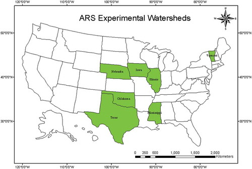
For this study, a set of 114 USDA-ARS watersheds varying in size from 0.2 to 12 990.5 ha are selected. These records are a collection of rainfall–runoff observations from small agricultural watersheds in the USA. The rainfall–runoff data for various years are available online.¹ Out of 114 watersheds, 57 are used for developing the different relationships and remaining 57 are used for validation of these developed relationships; their locations are shown in Figs 1 and 2, respectively.

Figure 1. Locations of United States Department of Agriculture, Agricultural Research Service (USDA-ARS) experimental watersheds used to develop the relationships

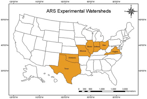
Figure 2. Location of ARS experimental watersheds used to validate the developed relationships

3.2 Determination of improved CN (CN_Imp)

The improved CNs (collectively CN_Imp) are determined using the following five steps, and their applicability conditions are also checked.

Step 1. Generate scatter plots for CN_T vs. CN_V using data for all 57 US watersheds.

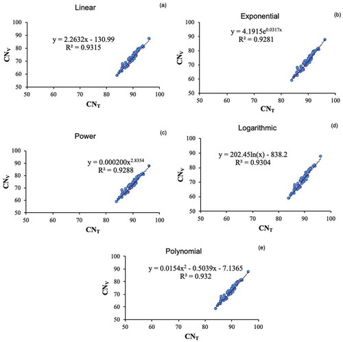
Step 2. Fit five different relationships (linear, exponential, power, logarithmic and polynomial) and determine R² for each relationship (see Fig. 3).

Figure 3. Scatterplots of CN derived from NEH-4 (CN_T) versus CN derived from Verma et al. (CN_V) for (a) linear, (b) exponential, (c) logarithmic, (d) power and (e) polynomial relationships

Step 3. Derive the improved CN (i.e. CN_Lin) for each watershed using CN_T and the developed linear relationship:

(16) $\mathrm{C}{\mathrm{N}}_{\mathrm{L}\mathrm{i}\mathrm{n}}=2.2632\mathrm{C}{\mathrm{N}}_{\mathrm{T}}-130.99$(16)

Step 4. Repeat steps 1–3 to similarly derive CN_Exp, CN_Pow, CN_Log and CN_Pol using exponential, power, logarithmic and polynomial functions, respectively, as follows:

(17) $\mathrm{C}{\mathrm{N}}_{\mathrm{E}\mathrm{x}\mathrm{p}}=4.1915\mathrm{e}\mathrm{x}\mathrm{p}\left(0.0317\right)$(17)

(18) $\mathrm{C}{\mathrm{N}}_{\mathrm{P}\mathrm{o}\mathrm{w}}=0.000200{\mathrm{C}\mathrm{N}}_{\mathrm{T}}^{2.8354}$(18)

(19) $\mathrm{C}{\mathrm{N}}_{\mathrm{L}\mathrm{o}\mathrm{g}}=202.45ln\mathrm{C}{\mathrm{N}}_{\mathrm{T}}-838.2$(19)

(20) $\mathrm{C}{\mathrm{N}}_{\mathrm{P}\mathrm{o}\mathrm{l}}=0.0154{\mathrm{C}\mathrm{N}}_{\mathrm{T}}^2-0.5039\mathrm{C}{\mathrm{N}}_{\mathrm{T}}-7.1365$(20)

Step 5. Calculate S using these CNs from Equation (5)(5) $S=\frac{25400}{\mathrm{C}\mathrm{N}}-254$(5) for computing runoff using the Verma et al. (2018) model. Tabular CN is also used to compute runoff using the original CN model (Equation 4(4) $Q=\{\begin{array}{l}\frac{{\left(P-I_a\right)}^2}{\left(P-I_a+S\right)}\text{for}P>I_a\\ 0\text{for}P\le I_a\end{array}$(4) ). These are described in Table 1.

3.3 Applicability of the proposed CN_Imp

The range of CN_T varies from 0 to 100 for estimating surface runoff, and so does the range of CN_Imp. More specifically, the proposed CN_Imp has its own applicability range limits. For example, CN_Lin varies from 0 (lower) to 95 (higher), which can be obtained if CN_T ≈ 58 and CN_T ≈ 100, respectively. This indicates that Equation (16)(16) $\mathrm{C}{\mathrm{N}}_{\mathrm{L}\mathrm{i}\mathrm{n}}=2.2632\mathrm{C}{\mathrm{N}}_{\mathrm{T}}-130.99$(16) is valid for 58 ≤ CN_T ≤ 100. Similarly, CN_Exp and CN_Pow vary from 4 to 100 and 0 to 94, respectively and can be obtained if 0 ≤ CN_T ≤ 100. CN_Log varies from 0 to 94, which can be obtained if 63 ≤ CN_T ≤ 100, whereas CN_Pol varies from 0 to 96, which can be obtained if 44 ≤ CN_T ≤ 100. These CN_Imp values are derivable from Equations (16(16) $\mathrm{C}{\mathrm{N}}_{\mathrm{L}\mathrm{i}\mathrm{n}}=2.2632\mathrm{C}{\mathrm{N}}_{\mathrm{T}}-130.99$(16) –18(18) $\mathrm{C}{\mathrm{N}}_{\mathrm{P}\mathrm{o}\mathrm{w}}=0.000200{\mathrm{C}\mathrm{N}}_{\mathrm{T}}^{2.8354}$(18) ), respectively.

3.4 Goodness of fit

From a practical or scientific viewpoint, hydrological models are usually aimed to reproduce measurements with satisfactory precision (Seibert 2001). Numerous statistical methods are used to assess a model’s performance quality. For assessing model performance in terms of prediction capability, three widely accepted statistical indices – the coefficient of determination (R²), the root mean square error (RMSE), and the Nash-Sutcliffe efficiency criterion (NSE; Nash and Sutcliffe 1970) – are used. These are mathematically expressed as follows:

(21) $R^2={\left[\frac{{\displaystyle {\sum }_{i=1}^N\left(Q_O-{\overline{Q}}_O\right)\left(Q_C-{\overline{Q}}_C\right)}}{{\displaystyle {\sum }_{i=1}^N{\left(Q_O-{\overline{Q}}_O\right)}_i^2\sum i=1N{\left(Q_C-{\overline{Q}}_C\right)}_i^2}}\right]}^2$(21)

(22) $\text{NSE}=\left[1-\frac{{\displaystyle {\sum }_{i=1}^N{\left(Q_O-Q_C\right)}_i^2}}{{\displaystyle {\sum }_{i=1}^N{\left(Q_O-{\overline{Q}}_O\right)}_i^2}}\right]\times 100$(22)

(23) $\mathrm{R}\mathrm{M}\mathrm{S}\mathrm{E}=\sqrt{\frac{1}{N}{\sum }_{i=1}^N{\left(Q_O-Q_C\right)}_i^2}$(23)

where Q_C is the computed runoff; Q_O is the observed runoff; ${\bar{Q}}_O$and ${\bar{Q}}_C$ are, respectively, the mean of observed and computed runoff values in a watershed; N is the total number of rainfall runoff events; and i is an integer varying from 1 to N.

4 Results and discussion

4.1 Computation of CN_Imp

The computed CNs using the developed relationships (Equations 16(16) $\mathrm{C}{\mathrm{N}}_{\mathrm{L}\mathrm{i}\mathrm{n}}=2.2632\mathrm{C}{\mathrm{N}}_{\mathrm{T}}-130.99$(16) –20(20) $\mathrm{C}{\mathrm{N}}_{\mathrm{P}\mathrm{o}\mathrm{l}}=0.0154{\mathrm{C}\mathrm{N}}_{\mathrm{T}}^2-0.5039\mathrm{C}{\mathrm{N}}_{\mathrm{T}}-7.1365$(20) ) for all 57 watersheds are listed in Appendix A, which shows that all CN_Imp (CN_Lin, CN_Exp, CN_Pow, CN_Log and CN_Pol) are close to CN_V, but far from CN_T. Among all CN_Imp values, CN_Lin, CN_Exp, CN_Log and CN_Pol appear very close to CN_V, whereas CN_Pow is comparatively far from CN_V.

4.2 Model comparison and performance evaluation

In this study, the computed runoff using all CNs is compared with the observed runoff. Furthermore, to assess the overall performance of the models, three goodness-of-fit measures i.e. R², NSE and RMSE, are used (Equations 21(21) $R^2={\left[\frac{{\displaystyle {\sum }_{i=1}^N\left(Q_O-{\overline{Q}}_O\right)\left(Q_C-{\overline{Q}}_C\right)}}{{\displaystyle {\sum }_{i=1}^N{\left(Q_O-{\overline{Q}}_O\right)}_i^2\sum i=1N{\left(Q_C-{\overline{Q}}_C\right)}_i^2}}\right]}^2$(21) –23(23) $\mathrm{R}\mathrm{M}\mathrm{S}\mathrm{E}=\sqrt{\frac{1}{N}{\sum }_{i=1}^N{\left(Q_O-Q_C\right)}_i^2}$(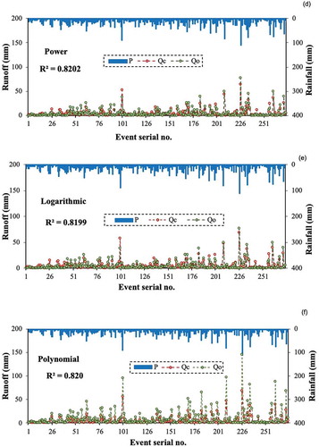23) ). The R² describes the proportion of the total variance in the observed data that can be explained by the model, and ranges from 0 to 1. Higher values of R² show superior performance, and decreasing values indicate a poor fit. A perfect correlation is obtained if R² = 1, and R² = 0 indicates no fit. Figure 4 shows the R² of all the models under study. For the watershed ID 44018, R² for linear, exponential, power, logarithmic, and polynomial models is 0.8199, 0.8197, 0.8202, 0.8199, and 0.82, respectively, values that are higher than those of the tabular model (0.7588). Similar results are obtained for the other watersheds (not shown for reasons of space).

Figure 4. Coefficient of determination (R²)-based comparative performance of (a) tabular, (b) linear, (c) exponential, (d) power, (e) logarithmic and (f) polynomial models for watershed ID 44018. P: rainfall; Qc: computed runoff; Qo: observed runoff

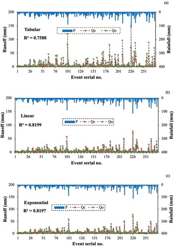
(Continued)

For performance evaluation and gradation of the models, R² was used as also recommended elsewhere (Santhi et al. 2001, Donigian 2002, Moriasi et al. 2012, 2015), and the results are shown in Table 2. According to the criterion of Santhi et al. (2001) (Table 2), the proposed models (linear, exponential, power, logarithmic and polynomial) show good fit in 48, 49, 46, 48 and 48 watersheds, respectively, whereas the tabular model shows good fit in 37 watersheds only. Similarly, according to the criteria of Donigian (2002) and Moriasi et al. (2012) (Table 2), the performance of the linear, exponential, power, logarithmic and polynomial models was, respectively, “very good” in 13, 12, 14, 13 and 13 watersheds, “good” in 19, 20, 19, 18 and 20 watersheds and “acceptable” in 16, 17, 13, 17 and 15 watersheds. In contrast, the tabular model does not perform very good in any watersheds, while “good” and “acceptable” fit is obtained in 23 and 14 watersheds, respectively. The tabular model is unsatisfactory in 20 watersheds, whereas the proposed model performance is unsatisfactory for a comparatively smaller number of watersheds. Similar results were obtained when the models were tested according to the criteria defined by Moriasi et al. (2015), further indicating the improved performance of the proposed models.

Table 1. Mathematical description of models under study. CN: curve number

Model	Method of CN estimation	Method of runoff computation
Tabular	NEH-4 table	Equation (4)(4) $Q=\{\begin{array}{l}\frac{{\left(P-I_a\right)}^2}{\left(P-I_a+S\right)}\text{for}P>I_a\\ 0\text{for}P\le I_a\end{array}$(4)
Linear	Equation (16)(16) $\mathrm{C}{\mathrm{N}}_{\mathrm{L}\mathrm{i}\mathrm{n}}=2.2632\mathrm{C}{\mathrm{N}}_{\mathrm{T}}-130.99$(16)	Equations (12(12) $\mathrm{I}\mathrm{f}P\le \left(0.12S-0.19S^{\ast }\right)\mathrm{t}\mathrm{h}\mathrm{e}\mathrm{n}Q=0$(12) –15(15) $S^{\ast }=\sqrt{P_{5}S}$(15) )
Exponential	Equation (17)(17) $\mathrm{C}{\mathrm{N}}_{\mathrm{E}\mathrm{x}\mathrm{p}}=4.1915\mathrm{e}\mathrm{x}\mathrm{p}\left(0.0317\right)$(17)	Equations (12(12) $\mathrm{I}\mathrm{f}P\le \left(0.12S-0.19S^{\ast }\right)\mathrm{t}\mathrm{h}\mathrm{e}\mathrm{n}Q=0$(12) –15(15) $S^{\ast }=\sqrt{P_{5}S}$(15) )
Power	Equation (18)(18) $\mathrm{C}{\mathrm{N}}_{\mathrm{P}\mathrm{o}\mathrm{w}}=0.000200{\mathrm{C}\mathrm{N}}_{\mathrm{T}}^{2.8354}$(18)	Equations (12(12) $\mathrm{I}\mathrm{f}P\le \left(0.12S-0.19S^{\ast }\right)\mathrm{t}\mathrm{h}\mathrm{e}\mathrm{n}Q=0$(12) –15(15) $S^{\ast }=\sqrt{P_{5}S}$(15) )
Logarithmic	Equation (19)(19) $\mathrm{C}{\mathrm{N}}_{\mathrm{L}\mathrm{o}\mathrm{g}}=202.45ln\mathrm{C}{\mathrm{N}}_{\mathrm{T}}-838.2$(19)	Equations (12(12) $\mathrm{I}\mathrm{f}P\le \left(0.12S-0.19S^{\ast }\right)\mathrm{t}\mathrm{h}\mathrm{e}\mathrm{n}Q=0$(12) –15(15) $S^{\ast }=\sqrt{P_{5}S}$(15) )
Polynomial	Equation (20)(20) $\mathrm{C}{\mathrm{N}}_{\mathrm{P}\mathrm{o}\mathrm{l}}=0.0154{\mathrm{C}\mathrm{N}}_{\mathrm{T}}^2-0.5039\mathrm{C}{\mathrm{N}}_{\mathrm{T}}-7.1365$(20)	Equations (12(12) $\mathrm{I}\mathrm{f}P\le \left(0.12S-0.19S^{\ast }\right)\mathrm{t}\mathrm{h}\mathrm{e}\mathrm{n}Q=0$(12) –15(15) $S^{\ast }=\sqrt{P_{5}S}$(15) )

Table 2. Model performance based on coefficient of determination (R²). Exp.: exponential; Log.: logarithmic; Poly.: polynomial

Reference	Category	Range	Model
			Linear	Exp.	Power	Log.	Poly.	Tabular
Santhi et al. 2001	Good	>0.60	48	49	46	48	48	37
	Poor	<0.60	9	8	11	9	9	20
Donigian 2002 and Moriasi et al. 2012	Very good	>0.80	13	12	14	13	13	0
	Good	0.70–0.80	19	20	19	18	20	23
	Acceptable	0.60–0.70	16	17	13	17	15	14
	Unsatisfactory	<0.60	9	8	11	9	9	20
Moriasi et al. 2015	Very good	>0.85	0	0	0	0	0	0
	Good	0.75–0.85	25	25	24	25	25	12
	Acceptable	0.60–0.75	23	24	22	23	23	25
	Unsatisfactory	<0.60	9	8	11	9	9	20

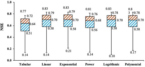
According to Ahmadisharaf et al. (2019), the R² criterion is unresponsive to additive and proportional differences between the simulated and observed values, but is more responsive to outliers than to the values near the mean, which could lead to a bias towards the extreme values. To overcome the limitations associated with the use of R², an alternative measure of goodness of fit, i.e. NSE, is used. The NSE compares the variance of the errors against the observations and varies from −∞ to 1. NSE = 1 is the optimum value, indicating that the observed vs. simulated data perfectly fit the 1:1 line. Values between 0 and 1 are generally considered acceptable, but with varying levels of performance, whereas values <0 indicate unacceptable performance – i.e. the model cannot predict better than the mean observed value. The NSE values for all the models under study are listed in Appendix B. Figure 5 presents a box-and-whisker plot comparing the models in terms of their performance based on NSE. The mean, median, and inter-quartile range of NSE for linear, exponential, power, logarithmic, and polynomial models is higher than the tabular model statistic.

Figure 5. Box-and-whisker plot of Nash-Sutcliffe efficiency (NSE) of the models under study

Performance is also evaluated according to the NSE grades, as shown in Table 3. According to the grading system of Santhi et al. (2001), the linear, exponential, power, logarithmic, and polynomial models exhibit satisfactory performance in 55, 55, 54, 55, and 56 watersheds, respectively, whereas the tabular model shows satisfactory performance in only 43 watersheds. When the performance is judged according to the criteria of Moriasi et al. (2007), the linear, exponential, power, logarithmic, polynomial and tabular models show very good performance in 23, 23, 24, 23, 23 and 5 watersheds, respectively, which indicates the improved performance of the proposed models over the tabular model. Unsatisfactory performance of the proposed models for a comparatively smaller number of watersheds also indicates their improved performance. Similar results were obtained when the models were tested according to the criteria of Moriasi et al. (2015). Furthermore, according to the criteria of Ritter and Mu~noz-Carpena (2013), the linear, exponential, power, logarithmic, polynomial, and tabular models showed acceptable performance in 28, 27, 27, 28, 28, and 26 watersheds, respectively, and good performance in 10, 11, 12, 10, 11, and 0 watersheds, respectively. None of the models showed very good performance in any watershed. The tabular model showed unsatisfactory performance in 31 watersheds, whereas the linear, exponential, power, logarithmic, and polynomial models showed unsatisfactory performance in 19, 19, 18, 19, and 19 watersheds, respectively, indicating the enhanced performance of all the proposed models.

Table 3. Model performance based on Nash-Sutcliffe efficiency criterion (NSE). Exp.: exponential; Log.: logarithmic; Poly.: polynomial

Reference	Grade	Range	Model
			Linear	Exp.	Power	Log.	Poly.	Tabular
Santhi et al. 2001	Satisfactory	>0.50	55	55	54	55	56	43
	Unsatisfactory	≤0.50	2	2	3	2	1	14
Moriasi et al. 2007	Very good	>0.75	23	23	24	23	23	5
	Good	0.65–0.75	15	15	15	15	16	21
	Acceptable	0.50–0.65	17	17	15	17	17	17
	Unsatisfactory	<0.50	2	2	3	2	1	14
Ritter and Mu~noz-Carpena 2013	Very good	>0.90	0	0	0	0	0	0
	Good	0.80–0.90	10	11	12	10	11	0
	Acceptable	0.65–0.80	28	27	27	28	28	26
	Unsatisfactory	< 0.65	19	19	18	19	18	31
Moriasi et al. 2015	Very good	> 0.80	10	11	12	10	11	0
	Good	0.70–0.80	21	20	19	21	20	19
	Acceptable	0.50–0.70	24	24	23	24	25	24
	Unsatisfactory	< 0.50	2	2	3	2	1	14

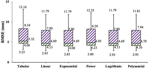
The RMSE provides an estimate of the error between the simulated and observed data. A higher value of RMSE indicates inferior model performance and vice versa. A perfect agreement between the observed and the computed value is obtained if RMSE = 0. The RMSE values for all the models under study are listed in Appendix B. Figure 6 shows the comparison of model performance on the basis of RMSE. The mean, median, and inter-quartile range of RMSE for linear, exponential, power, logarithmic, and polynomial models is lower than the RMSE statistics for the tabular model. The results thus indicate that all the proposed models (linear, exponential, power, logarithmic, and polynomial) perform equally well.

Figure 6. Box-and-whisker plot of root mean square error (RMSE) of the models under study

5 Conclusions

This study presented a procedure to determine improved curve numbers, CN_Imp (viz. CN_Lin, CN_Exp, CN_Pow, CN_Log and CN_Pol) using CN_T and five different mathematical relationships for estimating more accurate surface runoff. The CN_Imp values were found to be close to the CN_V values and very different from CN_T when their performance was tested on 57 USDA-ARS watersheds. The proposed models are found to be superior to the tabular model, as evidenced by higher R² and NSE statistics and lower RMSE statistics, as well as by visual assessment. Despite the fact that all of the proposed models performed almost equally well based on R², RMSE, and NSE statistics, the proposed models can be used for enhanced runoff prediction using the tabulated NEH-4 CN values. This underscores the efficacy of the Verma et al. (2018) model in improved runoff estimation for ungauged watersheds.

Acknowledgements

The authors are thankful to the anonymous reviewers, as well as to the associate editor, Professor Nikolaos Malamos, for their encouraging comments which helped to improve the article.

Disclosure statement

No potential conflict of interest was reported by the authors.

Notes

¹ http://www.ars.usda.gov/arsdb.html and http://hydrolab.arsusda.gov/arswater.html

Appendix A

Curve numbers (CN) obtained using the developed relationships. WS: watershed.

Table

WS ID	Area (ha)	Number of storms	CNT	CNV	CNLin	CNExp	CNPow	CNLog	CNPol
42016	8.4	293	86.35	67.31	64.44	64.74	61.82	64.40	64.18
42017	7.5	237	91.09	75.78	75.16	75.23	71.93	75.22	74.74
42023	1.31	80	92.79	80.63	79.01	79.40	75.80	78.97	78.70
42024	1.2	252	93.54	82.10	80.71	81.31	77.55	80.60	80.47
42028	1.2	263	92.8	79.47	79.03	79.43	75.83	78.99	78.72
42035	1.3	163	91.21	76.18	75.44	75.52	72.20	75.49	75.02
42036	1.3	197	91.63	77.35	76.39	76.53	73.15	76.42	75.99
42037	4.6	181	88.77	73.16	69.91	69.90	66.86	70.00	69.49
42038	2.3	158	89.3	73.92	71.11	71.08	67.99	71.21	70.67
42039	4	237	87.96	69.47	68.08	68.13	65.14	68.14	67.69
42040	4.6	226	87.98	69.17	68.13	68.17	65.18	68.19	67.73
44001	194.7	407	89.86	71.73	72.38	72.36	69.21	72.47	71.94
44002	166.3	482	86.65	65.69	65.12	65.36	62.43	65.11	64.83
44003	844.2	235	87	66.75	65.91	66.09	63.15	65.92	65.59
44004	1412.4	349	84.85	62.61	61.04	61.73	58.82	60.86	60.98
44007	1.5	524	94.13	82.11	82.05	82.85	78.95	81.87	81.88
44008	1.5	515	93.73	80.86	81.14	81.80	78.00	81.01	80.93
44009	1.6	537	91.21	75.04	75.44	75.52	72.20	75.49	75.02
44010	1.6	537	91.96	76.68	77.13	77.34	73.90	77.15	76.76
44011	1.7	486	90.63	74.03	74.12	74.15	70.91	74.20	73.69
44012	1.59	355	88.79	69.63	69.96	69.94	66.90	70.05	69.53
44014	1.6	262	89.22	70.55	70.93	70.90	67.82	71.02	70.49
44015	1.6	295	92.6	77.92	78.58	78.92	75.36	78.55	78.25
44016	1.5	309	93.23	79.23	80.01	80.52	76.83	79.92	79.74
44017	1.4	276	92.02	76.99	77.27	77.49	74.03	77.28	76.90
44018	1.4	274	92.71	78.50	78.83	79.20	75.62	78.79	78.51
44019	1.5	303	93.6	79.96	80.85	81.47	77.69	80.73	80.62
44020	1.4	281	93.23	79.73	80.01	80.52	76.83	79.92	79.74
44021	1.6	321	93.18	79.64	79.89	80.39	76.71	79.82	79.62
44022	1.5	320	88.1	68.95	68.40	68.43	65.44	68.47	68.00
44023	1.7	258	92.63	78.93	78.65	79.00	75.43	78.62	78.32
44024	1.6	264	90	73.33	72.70	72.68	69.52	72.79	72.25
44025	1.6	238	91.21	75.91	75.44	75.52	72.20	75.49	75.02
44026	1.5	241	92.34	77.08	77.99	78.28	74.76	77.98	77.64
44028	1.8	269	92.68	78.05	78.76	79.12	75.55	78.73	78.44
61003	157.8	463	85.08	62.06	61.56	62.18	59.27	61.41	61.47
62001	809.37	236	78.4	54.62	46.44	50.32	47.01	44.85	48.01
62002	404.7	136	90.74	76.00	74.37	74.40	71.15	74.44	73.94
62003	2237.9	28	89.03	69.86	70.50	70.48	67.41	70.59	70.07
62004	9226.9	22	89.82	69.10	72.29	72.27	69.12	72.38	71.84
62005	12 990.5	92	78.83	59.33	47.42	51.01	47.74	45.96	48.84
62010	8093.7	104	88.65	71.12	69.64	69.63	66.60	69.73	69.22
62012	3055.4	35	87.58	67.30	67.22	67.31	64.35	67.27	66.85
62014	0.6	134	94.93	84.82	83.86	84.97	80.86	83.58	83.81
62017	1295	26	89.04	67.56	70.53	70.50	67.43	70.62	70.09
62018	441.1	59	89.35	70.97	71.23	71.20	68.10	71.32	70.78
67005	11 116.4	247	79.01	55.01	47.83	51.30	48.05	46.42	49.19
69030	7.2	161	83.57	62.30	58.15	59.28	56.34	57.78	58.31
69032	17.9	198	89.7	72.00	72.02	71.99	68.86	72.11	71.57
69033	12.1	156	88.64	70.07	69.62	69.61	66.58	69.70	69.20
69035	5.26	116	85	64.06	61.38	62.03	59.12	61.21	61.30
69036	10.7	113	84.84	62.87	61.02	61.71	58.80	60.83	60.96
69042	9.6	85	76.94	53.30	43.14	48.04	44.57	41.05	45.26
69044	7.8	225	90.81	74.80	74.53	74.57	71.31	74.60	74.10
69045	11.1	250	86.91	67.26	65.70	65.90	62.96	65.71	65.39
70008	3.5	23	87.71	68.38	67.52	67.59	64.62	67.57	67.14
71002	33.51	1120	79.85	56.00	49.73	52.68	49.52	48.56	50.82

Appendix B

Root mean square error (RMSE) and Nash-Sutcliffe efficiency criterion (NSE) of all the models under study. WS: watershed.

Table

WS ID	RMSE						NSE
	Tabular	Linear	Exponential	Power	Logarithmic	Polynomial	Tabular	Linear	Exponential	Power	Logarithmic	Polynomial
42016	7.37	6.21	6.19	6.52	6.22	6.24	61.35	71.80	72.04	68.93	71.77	71.57
42017	9.14	8.02	8.02	8.34	8.02	8.04	69.05	75.26	75.28	73.28	75.28	75.13
42023	12.76	11.71	11.67	12.35	11.71	11.75	71.92	74.23	74.41	71.35	74.20	74.05
42024	11.23	10.78	10.76	11.10	10.79	10.80	58.60	60.97	61.17	58.65	60.92	60.86
42028	10.32	9.39	9.39	9.64	9.40	9.41	59.64	65.36	65.42	63.55	65.35	65.28
42035	13.16	11.79	11.79	12.07	11.79	11.81	49.12	58.21	58.24	56.24	58.23	58.07
42036	11.54	10.36	10.35	10.64	10.36	10.38	49.62	58.10	58.15	55.83	58.11	57.94
42037	7.81	7.32	7.32	7.75	7.31	7.37	70.37	72.38	72.37	69.05	72.45	72.01
42038	10.77	10.10	10.11	10.59	10.09	10.16	63.91	66.62	66.59	63.31	66.69	66.26
42039	9.72	8.03	8.03	8.29	8.02	8.05	52.79	66.04	66.06	63.76	66.07	65.83
42040	11.01	9.06	9.06	9.29	9.06	9.08	44.11	60.22	60.24	58.23	60.24	60.05
44001	5.07	4.25	4.25	4.38	4.25	4.26	66.80	76.46	76.46	75.02	76.47	76.42
44002	4.23	3.41	3.40	3.60	3.41	3.42	74.26	83.14	83.24	81.19	83.14	83.01
44003	5.26	4.54	4.53	4.85	4.54	4.56	72.92	79.52	79.63	76.65	79.53	79.29
44004	4.66	3.90	3.85	4.10	3.91	3.90	71.19	79.64	80.09	77.40	79.50	79.59
44007	4.92	4.56	4.56	4.74	4.56	4.56	74.19	77.64	77.65	75.82	77.61	77.61
44008	5.32	4.77	4.78	4.92	4.77	4.77	75.32	79.90	79.86	78.62	79.89	79.88
44009	4.33	3.80	3.80	3.93	3.80	3.80	75.82	81.17	81.18	79.81	81.17	81.12
44010	4.92	4.22	4.22	4.34	4.22	4.23	59.72	70.02	70.02	68.40	70.02	69.98
44011	5.01	4.34	4.34	4.46	4.34	4.34	57.14	67.49	67.50	65.66	67.51	67.39
44012	4.61	4.13	4.13	4.24	4.13	4.13	64.60	71.20	71.20	69.58	71.21	71.11
44014	5.44	4.48	4.48	4.57	4.48	4.49	40.24	58.20	58.19	56.47	58.21	58.11
44015	4.93	4.31	4.31	4.43	4.31	4.31	68.78	75.57	75.54	74.21	75.57	75.57
44016	5.89	5.02	5.03	5.11	5.02	5.02	54.91	66.56	66.48	65.41	66.57	66.57
44017	4.84	3.66	3.66	3.83	3.66	3.67	69.44	81.86	81.86	80.17	81.86	81.81
44018	4.92	3.93	3.94	4.10	3.93	3.94	71.77	81.31	81.30	79.69	81.31	81.28
44019	5.11	4.15	4.16	4.23	4.15	4.14	61.97	74.17	73.99	73.07	74.18	74.19
44020	4.48	3.99	3.99	4.16	3.99	3.99	75.95	80.08	80.06	78.35	80.08	80.06
44021	4.68	3.98	3.98	4.13	3.98	3.98	72.13	79.29	79.27	77.71	79.28	79.26
44022	5.19	4.16	4.16	4.30	4.16	4.17	50.78	68.01	68.03	65.90	68.04	67.85
44023	4.52	4.09	4.08	4.32	4.09	4.10	76.77	80.34	80.40	78.04	80.33	80.24
44024	5.52	4.69	4.69	4.83	4.69	4.70	41.28	56.22	56.21	53.59	56.25	56.01
44025	5.36	4.82	4.81	5.01	4.81	4.83	63.94	69.77	69.80	67.34	69.79	69.61
44026	5.44	4.33	4.34	4.43	4.33	4.33	65.78	77.37	77.32	76.29	77.37	77.40
44028	5.38	4.38	4.38	4.50	4.38	4.38	69.51	79.18	79.14	77.99	79.18	79.19
61003	3.38	2.93	2.92	3.00	2.93	2.93	43.06	56.76	57.04	54.79	56.67	56.70
62001	4.40	4.17	3.64	4.09	4.43	3.94	70.59	73.17	79.54	74.27	69.80	76.09
62002	8.34	7.90	7.90	8.38	7.90	7.94	77.42	79.23	79.24	76.64	79.26	79.00
62003	9.08	7.65	7.65	7.86	7.65	7.66	44.84	57.05	57.05	54.66	57.05	56.97
62004	7.34	5.91	5.90	5.79	5.91	5.86	39.74	54.30	54.34	56.00	54.15	54.97
62005	9.43	10.13	9.19	10.04	10.55	9.74	53.52	44.72	54.55	45.70	40.12	48.88
62010	9.93	8.82	8.82	9.26	8.81	11.05	70.26	75.81	75.81	73.30	75.85	61.98
62012	10.13	8.53	8.53	8.71	8.53	8.54	36.75	52.15	52.17	50.16	52.16	52.02
62014	7.33	6.76	6.71	7.18	6.78	6.76	73.08	76.67	76.95	73.61	76.52	76.64
62017	8.66	8.47	8.47	8.42	8.48	8.44	51.99	51.66	51.68	52.25	51.59	51.96
62018	8.08	6.43	6.43	6.59	6.43	6.44	43.55	62.95	62.95	61.15	62.96	62.85
67005	3.57	3.44	3.30	3.43	3.51	3.38	13.54	13.86	20.85	14.38	10.47	16.87
69030	4.62	3.84	3.76	4.00	3.87	3.83	55.15	68.62	69.96	65.98	68.13	68.82
69032	4.15	4.23	4.23	4.42	4.23	4.24	73.34	71.78	71.77	69.15	71.81	71.60
69033	4.84	4.94	4.94	5.14	4.94	4.96	67.95	65.73	65.73	62.87	65.77	65.50
69035	5.51	5.37	5.33	5.53	5.38	5.37	46.74	47.77	48.46	44.57	47.58	47.67
69036	5.15	4.78	4.74	4.95	4.79	4.78	49.58	55.59	56.31	52.34	55.37	55.52
69042	4.85	6.16	5.60	5.98	6.43	5.90	57.64	29.20	41.53	33.21	22.81	35.04
69044	4.45	3.66	3.66	3.92	3.66	3.68	73.38	81.69	81.70	79.04	81.71	81.52
69045	3.46	3.15	3.14	3.37	3.15	3.17	74.27	78.38	78.53	75.26	78.39	78.12
70008	7.85	8.48	8.48	8.69	8.48	8.50	58.48	47.61	47.65	44.94	47.63	47.38
71002	3.23	2.99	2.85	3.00	3.06	2.93	49.43	59.31	63.12	58.99	57.47	60.86

References

- Ahmadisharaf, E., et al., 2019. Calibration and validation of watershed models and advances in uncertainty analysis in TMDL Studies. Journal of Hydrologic Engineering, 24 (7), 3119001. doi:10.1061/(ASCE)HE.1943-5584.0001794
- Ajmal, M., et al., 2015. Evolution of a parsimonious rainfall–runoff model using soil moisture proxies. Journal of Hydrology, 530, 623–633. doi:10.1016/j.jhydrol.2015.10.019
- Banasik, K., et al., 2014. Curve number estimation for small urban catchment from recorded rainfall-runoff events. Archives of Environmental Protection, 40 (4), 75–86. doi:10.2478/aep-2014-0032
- Caletka, M., et al., 2020. Improvement of SCS-CN initial abstraction coefficient in the Czech Republic: a study of five catchments. Water, 12 (7), 1964. doi:10.3390/w12071964
- Donigian, A., 2002. Watershed model calibration and validation: the HSPF experience. Proceedings of the Water Environment Federation, 8 (8), 44–73. doi:10.2175/193864702785071796
- Hawkins, R.H., 1993. Asymptotic determination of runoff curve numbers from data. Journal of Irrigation and Drainage Engineering, ASCE, 119 (2), 334–345. doi:10.1061/(ASCE)0733-9437(1993)119:2(334)
- Hawkins, R.H., et al., 2002. Runoff curve number method: examination of the initial abstraction ratio. Proceedings of the Second Federal Interagency Hydrologic Modeling Conference. ASCE, Las Vegas, NV.
- Huang, M., et al., 2006. A modification to the soil conservation service curve number method for steep slopes in the Loess plateau of China. Hydrological Processes, 20 (3), 579–589. doi:10.1002/hyp.5925
- Lee, J.-Y., et al., 2019. Feasible ranges of runoff curve numbers for Korean watersheds based on the interior point optimization algorithm. KSCE Journal of Civil Engineering, 23 (12), 5257–5265. doi:10.1007/s12205-019-0901-9
- McCutcheon, S.C., 2006. Rainfall-runoff relationships for selected eastern U.S. forested mountain watersheds: testing of the curve number method for flood analysis. Technical Report, West Virginia Division of Forestry, Charleston, WV.
- Michel, C., Vazken, A., and Charles, P., 2005. Soil conservation service curve number method: how to mend among soil moisture accounting procedure? Water Resources Research, 41 (2), 1–6. doi:10.1029/2004WR003191
- Mishra, S.K., et al., 2006. An improved Ia-S relation incorporating antecedent moisture in SCS-CN methodology. Water Resources Management, 20 (5), 643–660. doi:10.1007/s11269-005-9000-4
- Mishra, S.K. and Singh, V.P., 2002. SCS-CN method: part I: derivation of SCS-CN based models. Acta Geophysica Polonica, 50 (3), 457–477.
- Moriasi, D.N., et al., 2007. Model evaluation guidelines for systematic quantification of accuracy in watershed simulations. Transactions of the American Society of Agricultural and Biological Engineers, 50, 885–900.
- Moriasi, D.N., et al., 2012. Hydrologic and water quality models: use, calibration, and validation. Transactions of the American Society of Agricultural and Biological Engineers, 55 (4), 1241–1247.
- Moriasi, D.N., et al., 2015. Hydrologic and water quality models: performance measures and evaluation criteria. Transactions of the American Society of Agricultural and Biological Engineers, 58 (6), 1763–1785.
- Nash, J.E. and Sutcliffe, J.V., 1970. River flow forecasting through conceptual models: part I- A discussion of principles. Journal of Hydrology, 10 (3), 282–290. doi:10.1016/0022-1694(70)90255-6
- Pandit, A. and Gopalakrishnan, G., 1996. Estimation of annual storm runoff coefficients by continuous simulation. Journal of Irrigation and Drainage Engineering, ASCE, 122 (4), 211–220. doi:10.1061/(ASCE)0733-9437(1996)122:4(211)
- Ponce, V.M. and Hawkins, R.H., 1996. Runoff curve number: has it reached maturity? Journal of Hydraulic Engineering, ASCE, 1 (1), 11–19. doi:10.1061/(ASCE)1084-0699(1996)1:1(11)
- Rallison, R.E. and Miller, N., 1982. Past, present and future SCS runoff procedure. Proceedings of international symposium on rainfall-runoff modeling. Littleton, Colordo: Water Resources Publications, 353–364.
- Ritter, A. and Mu~noz-Carpena, R., 2013. Performance evaluation of hydrological models: statistical significance for reducing subjectivity in goodness-of-fit assessments. Journal of Hydrology, 480, 33–45. doi:10.1016/j.jhydrol.2012.12.004
- Rutkowska, A., et al., 2015. Probabilistic properties of a curve number: A case study for small Polish and Slovak Carpathian Basins. Journal of Mountain Science, 12 (3), 533–548.
- Sahu, R.K., et al., 2007. An advanced soil moisture accounting procedure for SCS curve number method. Hydrological Processes, 21 (21), 2827–2881. doi:10.1002/hyp.6503
- Santhi, C., et al., 2001. Validation of the swat model on a large RWER basin with point and nonpoint sources. Journal of the American Water Resources Association, 37 (5), 1169–1188. doi:10.1111/j.1752-1688.2001.tb03630.x
- Schneider, L.E. and McCuen, R.H., 2005. Statistical guideline for curve number generation. Journal of Irrigation and Drainage Engineering, 131 (3), 282–290. doi:10.1061/(ASCE)0733-9437(2005)131:3(282)
- SCS (Soil Conservation Service), 1972. National engineering handbook. Supplement A, Section 4, Chapter 10. Washington, DC: Soil Conservation Service, US Department of Agriculture.
- SCS (Soil Conservation Service), 1975. Urban hydrology for small watersheds. Technical Release 55. Washington, DC: U.S. Department of Agriculture.
- Seibert, J., 2001. On the need for benchmarks in hydrological modelling. Hydrological Processes, 15 (6), 1063–1064. doi:10.1002/hyp.446
- Singh, P.K., et al., 2010. An updated hydrological review on recent advancements in soil conservation service curve-number technique. Journal of Water and Climate Change, 1 (2), 118–134. doi:10.2166/wcc.2010.022
- Singh, P.K., et al., 2015. Development of a modified SMA based MSCS-CN model for runoff estimation. Water Resources Management, 29 (11), 4111–4127.
- Soulis, K.X., 2018. Estimation of SCS curve number variation following forest fires. Hydrological Sciences Journal, 63 (9), 1332–1346. doi:10.1080/02626667.2018.1501482
- Tedela, N.H., et al., 2012. Runoff curve numbers for 10 small forested watersheds in the mountains of the Eastern United States. Journal of Hydrologic Engineering, 17 (11), 1188–1198. doi:10.1061/(ASCE)HE.1943-5584.0000436
- Verma, S., et al., 2017a. An enhanced SMA based SCS-CN inspired model for watershed runoff prediction. Environmental Earth Sciences, 76 (21), 736. doi:10.1007/s12665-017-7062-2
- Verma, S., et al., 2017b. A revisit of NRCS-CN methodology and application of RS and GIS for surface runoff estimation. Hydrological Sciences Journal, 62 (12), 1891–1930. doi:10.1080/02626667.2017.1334166
- Verma, S., et al., 2018. Simplified SMA-inspired 1-parameter SCS-CN model for runoff estimation. Arabian Journal of Geosciences, 11 (15), 420. doi:10.1007/s12517-018-3736-7
- Verma, S., et al., 2020. Activation Soil Moisture Accounting (ASMA) for runoff estimation using Soil Conservation Service Curve Number (SCS-CN) method. Journal of Hydrology, 589, 125114. doi:10.1016/j.jhydrol.2020.125114
- Wang, X., Liu, T., and Yang, W., 2012. Development of a robust runoff-prediction model by fusing the Rational Equation and a modified SCS-CN method. Hydrological Sciences Journal, 57 (6), 1118–1140. doi:10.1080/02626667.2012.701305