Canopy interception estimates in a Norway spruce forest and their importance for hydrological modelling

ABSTRACT

This study presents a comparison of several interception modelling approaches and their impact on the simulation of discharge, soil moisture content and groundwater level using the Hydrologiska Byråns Vattenbalansavdelning (HBV)-light model. The study was based on 10-year measurements of interception loss in a mature Norway spruce forest. The interception modelled by the subtraction of the constant value from each individual rainfall event was proved to be the most efficient. The root mean square error (RMSE) between observed and simulated discharge increased by 5–6% compared to the reference model run, no differences in the soil moisture were observed and an increase in RMSE of 11% was observed concerning the groundwater level. The transpiration rate was overestimated by 3–5% on average. The study proved that even simple interception models can serve efficiently for hydrological modelling tasks focused on the simulation of particular water fluxes in forested catchments.

KEYWORDS:

• interception
• water balance
• HBV model
• Gash model
• evapotranspiration
• soil moisture

Editor A. Fiori Associate editor D. Penna

1 Introduction

Interception loss plays an important role in water balance. It expresses the amount of rainwater that is temporally stored on the surface of the canopy. Several studies (David et al. 2006, Magliano et al. 2019) have demonstrated that interception is an important factor influencing microclimates and the water balance as it affects the amount of rainfall reaching the ground and plays a role in regulating the tree transpiration rate (Hadiwijaya et al. 2020). Understanding the dynamic processes of interception is vital, especially in the field of forest hydrology as it applies to a noticeable portion of rainfall (Peng et al. 2014). However, interception is often not treated as a separate process in modelling practices (Savenije 2004, Gerrits et al. 2007).

As an important component of the water balance, an accurate estimation of interception is necessary. Its underrepresentation leads to a deterioration in the accuracy of other water balance components or even the total water budget in forests (Dohnal et al. 2014, Wang and Wang 2017). Most research has focused on studying rainfall partitioning to examine the interception rate (Llorens and Domingo 2007, Staelens et al. 2008, Zhang et al. 2016, Návar 2020). Several methods, such as micrometeorological methods (Rutter et al. 1975, Gash 1979), water balance methods (Pypker et al. 2005, Zhang et al. 2016) and direct weighing methods conducted under laboratory conditions (Mauch et al. 2008), have been tested for the determination of the proper rate.

In addition to the accuracy of different methods (Linhoss and Siegert 2016), researchers (Gerrits et al. 2007, Li et al. 2016) have discussed the influence of three groups of variables on the interception process: (1) tree species and their attributes (e.g. tree crown and leaf morphology) (Kermavnar and Vilhar 2017, Liu et al. 2018); (2) rainfall characteristics (e.g. rainfall intensity, duration and drop size; Nanko et al. 2006, Zabret et al. 2018); and (3) meteorological parameters (e.g. relative humidity and wind speed) (Van Stan et al. 2014, Zabret et al. 2018). Although there have been many interception studies focused on the thorough modelling of interception loss (summarized by Muzylo et al. 2009), its influence on the modelled water balance of forests has been (to our knowledge) insufficiently studied. The estimation of interception loss is a standard part of most hydrological models that is used for the determination of throughfall from the gross rainfall measured in the open area, which is normally available from standard meteorological stations. Nevertheless, the quantification of errors introduced by different interception estimation equations on the estimation of discharge, soil water regime, groundwater dynamics and the components of the catchment’s water balance is missing.

Therefore, this study focuses on quantifying interception, estimating it using various interception models and testing its predictive power in the water balance of spruce forests. We compared the results of the hydrological model using measured throughfall with simulations based on estimated throughfall amounts. The main aims of this study are therefore as follows: (1) to model interception loss by several simplistic approaches; and (2) to evaluate the effect of the variability associated with different estimates of interception on the simulated discharge, soil water, groundwater storage and water balance.

2 Materials and methods

2.1 Experimental site and data

The Liz catchment (49°04´N, 13°41´E) served as the experimental area for this study. The site is located in a mountainous and forested part of the Czech Republic and covers an area of 0.99 km². The average altitude is 941 m a.s.l., the average daily air temperature is 6.6°C, and the average annual precipitation is 863 mm. The long-term averages are from the measurement period extending from 1976 to 2018. The site is generally characterized by a humid continental climate belonging to the Dfb climate zone according to the Köppen climate classification system (Tolasz et al. 2007). Forest cover on the throughfall measurement plot is formed by 120- to 130-year-old Norway spruce (Picea abies (L.) Karst.) with an average height of approximately 28 m and a mean diameter of 38 cm (for details, see Dohnal et al. 2014).

The measurements taken for this experiment included air temperature (Fiedler RV12/RK5, Czech Republic), global radiation (Kipp & Zonen CMP3, Netherlands) and soil moisture content (Campbell CS616, United States). Soil moisture was measured to a depth of 80 cm at 10-cm intervals. The column average soil moisture content was calculated as the arithmetic average. The precise location of soil moisture measurement was chosen to represent the average age of the forest, the average hillslope angle and the approximate average altitude within the catchment. Moreover, the experimental area was equipped with instruments measuring the discharge and groundwater level. All aforementioned data were measured at 10-min intervals.

The gross rainfall (P_G) was measured with a weighing raingauge at a meteorological station outside the forest, located approximately 300 m from the throughfall measurement locations. Throughfall was measured with a set of four tipping-bucket raingauges (Fiedler SR03, Czech Republic) in the same time steps as the P_G. The measurement accuracy of both types of raingauges was ± 0.1 mm. The raingauges were placed randomly under forest canopy, and the canopy biometric characteristics and measurements of crown closure were thoroughly described by Dohnal et al. (2014). One raingauge was placed near the stem, two raingauges were placed in the dripping zone (i.e. under tree branches, representing the most common area according to crown closure) and one was placed in the forest windows. Throughfall data were collected from June 2009 to November 2018. Dohnal et al. (2014) previously reported that the stemflow accounted for up to 1% of the gross rainfall at the inspected site; hence, it was neglected in this study. Interception was primarily determined on a monthly basis as the difference between the sums of the P_G and the average throughfall amount from all four tipping-bucket raingauges. The estimation of snow interception was based on manual measurements of snow depth regularly conducted 3 times a week during all winter seasons (November–April). The abovementioned measurements were conducted both under the forest canopy and in a nearby opening. A linear regression was used for the transformation of open area to under-canopy snowfall to obtain a continuous record. The long-term average ratio between the forested site and open-area snow depth was 0.59 (R² = 0.78), which was used for the continuous estimation of net snowfall, and the remaining 41% was assumed to be intercepted by the forest canopy. An explanation of the method and more information about snow measurements are available in a study by Šípek and Tesař (2014). Side experiments performed using the degree-day method showed that the long-term annual fraction of total precipitation that fell as snowfall was approximately 17%, which is in line with the results (13–24%) obtained by Jeníček and Ledvinka (2020) for nearby catchments.

Subsequently, an analysis of daily interception in individual rainfall events was conducted. However, due to methodological difficulties, a significant number of events were omitted from the final analyses. First, we omitted the events when the P_G was lower than 0.5 mm, as it was in most cases where no throughfall was observed. These events accounted for 223 out of 978 detected rainfall events during the 10 investigated summer periods (altogether accounting for less than 1% of the total rainfall). Second, due to the daily time step chosen for this study, we omitted events in which the same rainfall event was observed over several consecutive days. In these events, the intercepted amount could have been biased due to interevent evaporation or the split of rainfall and throughfall into 2 d (when midnight was passed). This accounted for the exclusion of an additional 212 events, which made up 24% of the total rainfall amount over the 10 inspected summer periods. As a result, the analysis of daily interception was conducted on 543 events, which represented 75% of the total rainfall amount. A Kolmogorov-Smirnov test proved that there was no statistically significant difference in the probability distribution of gross rainfall in the 543 analysed events versus the 212 events that were excluded due to the daily time step. Hence, the exclusion of the latter should not have had a substantial influence on the analysis.

2.2 Hydrological model

The hydrological model used was the Hydrologiska Byråns Vattenbalansavdelning (HBV)-light rainfall–runoff model (Bergström 1992, Seibert and Vis 2012). This is a semi-distributed model utilizing several elevation zones that works in a daily time step. The model setup using three groundwater boxes was selected. These were the top groundwater zone (STZ), upper zone (SUZ) and lower zone (SLZ) boxes. All zones were gradually connected by percolation. Input into the STZ is represented by the portion of precipitation that is not stored in soil. This partition is governed by soil moisture and its changes over time (a higher portion of precipitation percolates to the STZ as the soil saturation increases). The basic equations describing individual routines are available in studies by Seibert (1997) and Seibert and Vis (2012).

The necessary input data comprised daily sums of precipitation, air temperature and potential evapotranspiration (PET). The PET was estimated by the Penman-Monteith approach (Monteith 1965) using a site-specific calibration in the net longwave radiation equation (Kofroňová et al. 2019). The model parameters were calibrated using a genetic algorithm and Powell optimization (GAP) with the Nash-Sutcliffe estimate to serve as an objective function (Seibert 2000).

Altogether, 12 model parameters were calibrated within the ranges recommended in the model instructions (Table 1). They included three parameters necessary to estimate snow accumulation and snowmelt. These were the threshold temperature, which divides snowfall from rainfall and snowmelt from accumulation (TT, °C); the snow melt rate (CFMAX, mm/Δt °C); and the snowfall correction factor (SFCF, dimensionless). Three parameters were used for the soil moisture routine: field capacity (FC, mm), the soil moisture value above which actual evapotranspiration (AET) reaches PET (LP, mm) and the parameter that determines the relative contribution of rain or snowmelt to runoff (BETA, dimensionless). The remaining six parameters were used to estimate the contribution of groundwater to the total runoff. The three dimensionless storage coefficients K0, K1 and K2 were used for the estimation of drainage volume from the three groundwater boxes. Two coefficients determined the maximum rate of percolation to the upper (UZL, mm/Δt) and lower (PERC, mm/Δt) groundwater zones. Finally, a single coefficient was necessary for the triangular weighted transformation of runoff (MAXBAS, Δt).

Table 1. Values and ranges of parameters obtained from the reference calibration. AVG stands for the average value of the parameter and SD represents its standard deviation. Parameter labels are explained in section 2.2

Parameter	Unit	Range		All calibrations	22 best runs	Best set
		Min	Max	AVG ± SD	AVG ± SD	Value
PERC	mm/Δt	0	inf	2.97 ± 0.77	1.87 ± 0.22	1.53
UZL	mm	0	inf	23.16 ± 10.11	8.82 ± 0.28	8.56
K0	1/Δt	0	1	0.11 ± 0.14	0.28 ± 0.01	0.29
K1	1/Δt	0	1	0.15 ± 0.04	0.08 ± 0.01	0.06
K2	1/Δt	0	1	0.01 ± 0.00	0.01 ± 0.00	0.01
MAXBAS	Δt	1	100	1.34 ± 0.23	1.67 ± 0.03	1.71
TT	°C	−inf	inf	−0.06 ± 0.10	−0.01 ± 0.08	0.00
CFMAX	mm/Δt°C	0	inf	1.23 ± 0.09	1.31 ± 0.09	1.31
SFCF	-	0	inf	1.50 ± 0.01	1.49 ± 0.02	1.47
FC	mm	0	inf	222.0 ± 5.5	226.1 ± 8.0	221.91
LP	-	0	1	0.90 ± 0.06	0.95 ± 0.03	1.00
BETA	-	0	inf	2.81 ± 0.36	2.92 ± 0.26	3.21

2.3 Interception modelling

Four simple approaches were utilized to estimate the amount of water intercepted by the tree canopy. One approach was applied in two different forms; hence, altogether, five time series of interception were examined (models A–E). The aim of this was to compare the observed interception amount with the estimated amount. Subsequently, all of the estimates (along with the observed throughfall) were used as input for the hydrological model. The model results were then compared to the observed values of discharge, volumetric soil moisture content and groundwater level to determine the influence of the chosen approach on the simulation of the particular variable. The chosen models were as follows:

• Model A employed the deduction of the maximum interception capacity of the canopy (threshold model) from each P_G. This approach is used, for example, in the Soil and Water Assessment Tool (SWAT) model (Arnold et al. 1993). The maximum interception capacity of the present spruce forest was determined by Dohnal et al. (2014) to be 2.1 mm.

• Model B used a multiplication approach, where the P_G was multiplied by a single coefficient so that the total interception amount simulated during the growing season corresponded to the observed values of 135 mm/season. In our case, a constant coefficient of 0.25 was used to determine the interception amount.

• Model C was similar to model B, but the multiplication coefficient was set according to Dohnal et al. (2014), who determined the long-term ratio between interception loss and P_G. A value of 0.35 was obtained in their 2-year experiment.

• Model D employed the power model approach as proposed by Návar (2020). The model parameters were obtained from the assessment of daily throughfall data from the 543 events over the entire inspected period by the minimization of the least square error (described more thoroughly in section 2.1).

• Model E followed the revised Gash model (Gash et al. 1995) for the sparse canopy, which is the most commonly used interception modelling approach (Muzylo et al. 2009). The interception loss in a revised Gash model is calculated as follows:

(1) ${\sum }_{j=1}^{n+m}{I}_j=c{{\sum }_{j=1}^m{P}_{G,j}+ncP{ }^{\mathrm{\prime }}}_G+c\frac{\overline{E_c}}{\bar{R}}{\sum }_{j=1}^n{(P_{G,j}-P{ }^{\mathrm{\prime }}}_G)+q{s}_t+p_t{\sum }_{j=1}^{n-q}{P}_{G,j}$(1)

where n and m are the numbers of days with sufficient and insufficient rainfall, respectively needed to saturate the canopy; q is the number of days with rainfall sufficient to saturate the trunks; I is the resulting interception loss (mm/t); c is the canopy cover (%); P_G is the gross rainfall (mm/t); P´_G is the amount of rainfall necessary to saturate the canopy (mm); $\overline{E_c}$ is the mean evaporation rate of the saturated canopy during the rainfall event per unit canopy area (mm/t), defined as $\overline{E_c}=\bar{E}/c$; $\bar{R}$ is the mean rainfall after canopy storage saturation (mm/t); s_t is the trunk storage capacity (mm/t); and p_t is the portion of rain diverted to the trunks (%).

The Gash model parameters were obtained from the event-based regression analyses (used e.g. by Pypker et al. 2005) of gross rainfall and throughfall data measured automatically in 15-min time intervals in 4 of the 10 years (2012, 2013, 2016, 2017; the first two were adopted from Dohnal et al. (2014)), which represented the beginning and end of the inspection period. Only storms preceded by a dry period with at least 8 h of daylight were considered for this purpose (Gash and Morton 1978), and the end of a storm was defined following the procedure outlined by Pearce and Rowe (1981). This meant that continuous storms were permitted to be interrupted by 1-h periods without rain if the storm duration was 4 h or less, and by 2-h periods without rain if the storm duration was longer than 4 h. A total of 67 storms with P_G > 2 mm were analysed, as they matched these criteria.

A clear change in the slope of the relationship between throughfall and gross rainfall (P_G) enabled the division of the rainfall data into two phases: before and after saturation of the canopy interception capacity. The threshold necessary to saturate canopy (P´_G) was defined as the point where this slope changed. The canopy cover (c) was taken as the slope of the regression (a) of interception loss versus gross rainfall for small rainstorms that were insufficient to saturate the canopy (P_G < P´_G) (first phase). The slope of the linear regression (b) in the second phase (P_G ≥ P´_G) was used to predict average rainfall evaporation in the specific event ($\bar{E}$) according to Carlyle-Moses and Gash (2011), using the equation $\bar{E}=b\cdot \bar{R}$. As stemflow was not measured, the two parameters expressing trunk evaporation were assumed to be equal to those reported for Norway spruce by Ringgaard et al. (2014).

2.4 Hydrological modelling procedure

The measured throughfall, along with the estimated snowfall interception, was used for the calibration of the reference hydrologic model (hereinafter referred to as the reference run). In the summer period, throughfall was taken directly from the four raingauges placed under the forest canopy, and in the winter, it was inferred from the open-area snowfall according to Šípek and Tesař (2014). Furthermore, interception in the growing season was estimated by the five simple modelling approaches (models A–E). These estimated interception amounts were used for model calibration, each relying on a different method of interception estimation, which refers to instances when no measured interception was available. This final step was split into two separate tasks. Initially, the estimated interception was used only for the growing season (May–October), and the winter interception was estimated in the same way as in the reference run (‘same winters’). Subsequently, the amount of winter interception was estimated using the five simple models (‘different winters”). The aim of the split was to differentiate the influence of the modelled interception in the two distinct seasons. Altogether, 11 calibration tasks were conducted: one reference run using the measured interception, five tasks using the estimated interception in the growing season and five tasks in which the interception was modelled for the entire year.

2.5 Model evaluation

The results of the different interception modelling approaches (models A–E) were compared to the observed interception loss. Subsequently, the results of the HBV model calculated with the different interception estimates as input were compared to the modelled results calculated with the observed interception. Seasonal and annual sums were thoroughly analysed using two statistical indicators evaluating the difference between the measured and estimated values: the root mean square error (RMSE) and Nash-Sutcliffe efficiency (NSE). RMSE tends to emphasize higher values of the error, whereas lower values are virtually neglected. RMSE is not bounded from above, and a value of 0 corresponds to a perfect fit. NSE is a dimensionless coefficient unbounded from below, and a maximum value of 1 corresponds to a perfect match in simulation.

3 Results

3.1 Climate characteristics and observed interception

The climatic characteristics during the examined period (2009–2018) are depicted in Fig. 1. The average air temperature of the 10 evaluated years was 7.4°C, and the mean annual precipitation in the given period was 757 mm/year. The most frequent precipitation events were events with up to 2 mm/d, accounting for 49% of all recorded rainfall events in the growing season (978 events in total over 10 years) but making up only 6% of the total rainfall amount. There was a visible increasing trend in the frequency of these rainfall events over the measured period. Similar changes were observed in the frequency of daily rainfall events of more than 15 mm/d. These increases in frequency were compensated by a lower frequency of precipitation between 2 and 15 mm/d.

Figure 1. Annual precipitation (P) and air temperatures (T) of the studied period (left panel) compared to long-term averages (P and T with avg subscript), and seasonal (May–October) amounts of precipitation and interception (right panel)

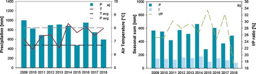
The annual observed interception losses are shown in Fig. 1 and Table 2. During the entire examination period, the mean annual interception in the growing season (May–October) equalled 135 mm, which means intercepted water constituted 29.1% of the measured precipitation. The lowest amount of intercepted water occurred during two years with the lowest observed gross rainfall, 2018 and 2015, with 93 and 96 mm of intercepted water (20 and 35% of the P_G), respectively. The maximum absolute intercepted amount (177 mm) occurred in the year 2014, accounting for 28% of the P_G. The highest sum of gross rainfall was observed in this year, indicating a direct relation between the gross rainfall and the amount of intercepted water.

Table 2. Monthly values of the measured P_G and interception, and their ratio

	2009	2010	2011	2012	2013	2014	2015	2016	2017	2018
Gross rainfall (PG) (mm)
May	na	122	91	23	116	138	76	69	52	78
June	243	99	99	132	163	37	63	139	49	153
July	141	155	90	152	21	217	26	154	60	64
August	63	114	57	171	127	135	30	65	88	54
September	45	44	27	51	45	80	41	109	54	90
October	75	18	57	45	44	57	50	71	69	50
Sum	567	551	421	574	516	665	286	606	373	490
Interception (mm)
May	na	26	17	3	38	46	26	20	4	5
June	52	12	28	39	31	15	19	37	21	26
July	38	37	34	39	11	50	11	38	30	19
August	19	41	23	44	37	38	11	17	21	13
September	14	14	6	16	23	20	18	17	15	19
October	21	9	19	18	13	8	11	20	31	11
Sum	143	139	127	160	153	177	96	149	121	93
Interception/PG (%)
May	na	21.1	19.1	14.0	32.4	33.3	34.8	28.8	8.0	5.8
June	21.3	11.8	28.5	29.5	18.8	41.9	30.5	26.6	42.3	17.0
July	26.9	23.9	37.9	25.6	53.0	22.8	42.2	24.7	49.2	29.6
August	29.6	35.9	40.0	26.0	29.3	28.3	37.4	26.6	23.5	24.8
September	30.0	32.7	22.5	31.8	51.7	24.7	42.7	15.5	27.4	21.1
October	28.3	52.5	32.8	40.9	29.1	14.8	20.9	28.7	44.9	21.8
Average	27.2	29.7	30.1	28.0	35.7	27.6	34.7	25.1	32.5	20.0

The intraseasonal variation in interception followed, on average, the same pattern as its annual variation. The highest interception amounts were observed in July and August when the P_G was also highest. The I/P_G ratio, on average, increased during the season, which could be attributed to the prevailing occurrence of events with higher precipitation (> 15 mm/d) at the beginning of the growing season.

The highest and lowest interception losses occurred in the same years as the highest and lowest precipitation amounts (in 2014 and 2015, respectively). An influence of the number of rainfall events exceeding a specific threshold (e.g. 10 mm/d) was also detected in the amount of interception loss. Specifically, the correlation coefficient between the I/P_G ratio and the ratio of > 10 mm/d precipitation events to all rainfall events was −0.91. This agreed with the observation that the interception rate decreased with an increase in the amount of precipitation in single rainfall events. In our case, the highest I/P_G ratio was achieved in 2013 (35.7%), when 52 of the 90 recorded precipitation events reported rainfall of less than 3 mm. The second highest I/P_G ratio was found in 2015 (34.7%), when 61 rainy days (out of the total of 89 d with rain, data not shown) with precipitation amounts of less than 3 mm occurred. In both years, the number of rainfall events with precipitation greater than 15 mm/d was also very low. The period average was 10 events (> 15 mm/d) per growing season; however, only three in 2015 and eight in 2013 were recorded.

Event-based regression analysis was conducted for 2016 and 2017 using 15-min rainfall records, which were supplemented with the results obtained by Dohnal et al. (2014) for 2012 and 2013. Altogether, 28 rain events that occurred in these two years were analysed. The characteristics of the particular rain events used are given in Table 3. The average values of the threshold (P´_G) factor were 2.4 mm in 2016 and 1.5 mm in 2017. Free throughfall equalled 30.7% of the total rainfall in 2016 and 26.2% in 2017. The average in-storm evaporation (E_c) was 0.25 mm/h in 2016 and 0.66 mm/h in 2017. The standard deviations equalled 0.22 mm/h and 0.65 mm/h. The corresponding values of E were 0.19 mm/h and 0.50 mm/h, respectively. The high variability of the reported values can be attributed to differences in the relative humidity of the air, wind velocity and rainfall characteristics (intensity and drop sizes). When the values were averaged together with the years investigated by Dohnal et al. (2014), the parameters for the revised Gash model were as follows: c = 0.77, P´_G = 2.1 mm, E_c = 0.57 mm/h and R = 1.9 mm/h; hence, E/R = 0.23. The trunk parameters were assumed to be equal to those reported by Ringgaard et al. (2014) who studied the the interception of mature spruce forest; hence, p_t = 0.011 and S_t = 0.034 mm, respectively.

Table 3. Characteristics of selected rainfall events in the Norway spruce forest in 2016–2017. THRG stand for throughfall. Missing values could not be determined reliably

		PG	Duration	P´G	Free THRG	E
		mm	min	mm	%	mm/h
2016	1	4.1	270	1.9	30.2	0.09
2016	2	14.0	460	1.6	30.5	0.09
2016	3	5.9	600	3.2	22.0	0.19
2016	4	5.8	280	1.7	26.3	0.07
2016	5	4.4	590	2.2	17.9	0.14
2016	6	10.0	410	1.5	16.7	0.34
2016	7	4.2	150	2.2	22.8	0.69
2016	8	3.5	300	0.8	25.9	0.27
2016	9	12.3	450	2.5	55.8	0.14
2016	10	7.2	320	1.3	44.0	0.03
2016	11	8.6	570	3.0	45.5	0.21
2016	12	7.6	360	1.3	25.5	0.00
2016	13	44.0	1300	9.0	29.2	0.31
2016	14	4.8	690	2.2	35.3	0.13
2016	15	13.0	520	3.3	45.8	0.19
2017	1	8	200	4.8	-	1.36
2017	2	8	190	3.0	-	0.70
2017	3	7.7	190	2.0	-	0.02
2017	4	9.3	300	1.8	-	0.37
2017	5	2.1	190	1.5	10.5	0.41
2017	6	18.4	270	4.6	-	1.64
2017	7	6.8	180	1.0	-	0.02
2017	8	15.2	590	1.6	35.7	0.11
2017	9	17	200	3.2	-	0.47
2017	10	19.4	310	5.4	-	0.71
2017	11	9	420	2.4	-	0.17
2017	12	2.8	390	1.5	32.6	0.11
2017	13	5.2	450	3.8	-	0.48

3.2 Interception estimates from different approaches

The interception loss for the period 2009–2018 was estimated using several modelling approaches (models A–E). Winter interception measurements are often problematic (Šípek and Tesař 2014). Therefore, the winter interception losses were first considered the same for all modelling approaches, and the interception amounts in the growing seasons were estimated separately. Then, the interception amounts in the winter seasons were also determined using models A–E.

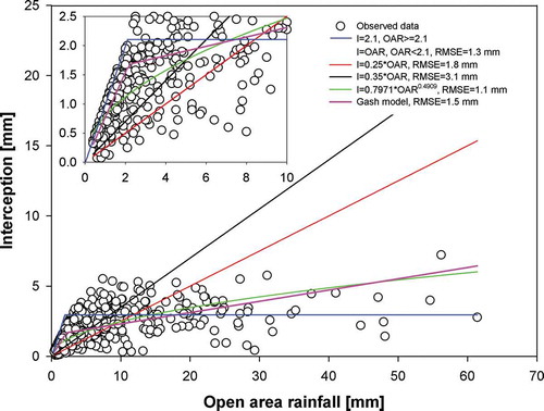
The daily values of interception and P_G are plotted in Fig. 2. Based on the procedure described in section 2.1, we analysed 543 events over the 10-year time period. It was obvious that none of the models based on either a linear or a power relationship (as proposed by Návar 2020) could reproduce the measured data sufficiently. This was mainly due to the high variability of individual throughfall events (caused by different meteorological conditions) and the chosen daily time step (given by the utilized hydrological model). Figure 2 documents the differences in the abilities of particular models to predict daily interception expressed as the RMSE, ranging from 1.1 to 3.1 mm. The method with the highest predictive power was the power model – Model D (RMSE = 1.1 mm), followed by the threshold model – Model A (RMSE = 1.3 mm), the Gash model – Model E (RMSE = 1.5 mm), the calibrated linear model without intercept – Model B (RMSE = 1.8 mm), and the simple linear model – Model C (RMSE = 3.1 mm).

Figure 2. Graphical representation of interception estimation (I) by utilized models compared to measured daily open area rainfall (OAR)

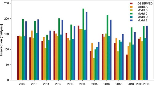
The average seasonal interception estimates modelled by the five proposed approaches are shown in Fig. 3 (growing seasons of 2009–2018). When compared to the observed interception loss, some methods estimated the process with significant differences. The average annual interception losses from the different modelling approaches reached values ranging from 112 to 177 mm/year. Altogether, models C and E were the least accurate of all methods in the whole period of examination; they overestimated the interception by, on average, 42 mm/year (Fig. 3). The worst performance of model C was also confirmed by the resulting RMSEs obtained from the comparison of monthly interception sums. The RMSE ranged from 6 mm (model D) to 12 mm (model C). The remaining RMSEs equalled 7–9 mm. The 2009–2018 interception totals were similar for the observations and model B, as the difference between their values was the objective function of their calibration.

Figure 3. Observed (OBS) interception loss in the growing season (May–October) compared with interception estimated by different modelling approaches (A–E)

Winter interception measurements are typically omitted in many studies. To consider the accuracy of the utilized modelling approaches, the decision was made to analyse the growing season separately. Then, the amount of interception loss during winter was evaluated with models A–E and compared. The lowest value of winter interception (November–April) was the output from model B, which reported 75 mm on average per winter season. The highest average values were reported when using models A and E; these were 125 and 129 mm, respectively. These values were close to the overall observed mean winter interception (122 mm) in the examined period. Models C and D attained, on average, interception values of 105 and 110 mm in the winter season, respectively.

3.3 Hydrological model calibration

The hydrological model was calibrated using the entire 10-year investigation period. The reason for this was that the separation of the total period into calibration and validation periods would not allow equal coverage of the wet and dry years in both periods, as the last 4 years were drier than the first 6 years. The importance of longer time series for model calibration has been stressed, e.g. by Larssen et al. (2007).

In the reference run (using the measured interception), the HBV model was calibrated 100 times. The threshold Nash-Sutcliffe coefficient was set to 0.75, which was exceeded 22 times out of all the conducted calibrations. The lowest NSE coefficient obtained was 0.72. The maximum efficiency was 0.77. Table 1 depicts the averaged values of calibrated parameters obtained in all 100 calibrations, the average parameter values obtained in the 22 best model runs (NSE > 0.75) and the best parameter set. The standard deviations of most parameters decreased when only the best 22 runs were selected, indicating the stability of the final model parameters.

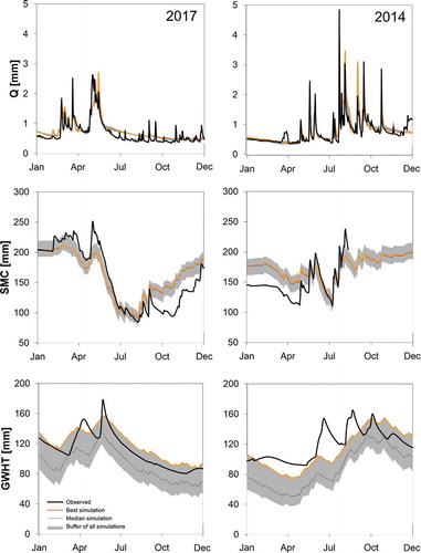
Furthermore, all 22 model parametrizations were inspected, and the differences between them were small in magnitude. In the case of runoff, the RMSE of all calibrations ranged from 0.36 to 0.37 mm/d (40–41% of the long-term average). The RMSE values were, in this case, caused by several peak flows that were not captured sufficiently (discussed later). The soil moisture content was estimated with RMSEs ranging from 26.5 to 44.3 mm (18–30% of the long-term average). Larger differences were found in the groundwater simulations when the RMSE values ranged from 17 to 38% of the long-term average. Nevertheless, the differences among these 22 model runs were mainly produced by the slight upwards or downwards shift of the simulated series from the observed series. This is supported by the stable value of the correlation coefficient between the observed and simulated datasets. The differences in the correlation coefficient were up to 0.02 (considering all 22 most efficient model runs) in the case of runoff and soil moisture content and 0.07 for the groundwater level estimation. The similarities of all 22 model runs are depicted in Fig. 4, which shows the observed and simulated values of runoff, soil moisture content and groundwater level for a dry year (2017) and a wet year (2014). Based on this, the single parameter set was used for the investigation of the interception estimation approach on model efficiency.

Figure 4. Spread of the 22 best calibrations of the HBV-light model displayed for discharge (Q), soil moisture content (SMC) and groundwater storage values (GWHT) in a wet year (2014) and in a dry year (2017)

The best parameter set resulted in an NSE coefficient of 0.77. The volume of runoff was, on average, underestimated by 1.9% in the 10-year period. The RMSE was 0.36 mm/d. Approximately one-fourth of the RMSE was produced by the incorrect prediction of six peak discharges (when these were omitted, the RMSE decreased to 0.30 mm/d). The NSE coefficient concerning the soil moisture estimation was 0.69, which also indicated the satisfactory prediction of soil saturation. The largest discrepancies were observed in a dormant season (October–April; see Fig. 4), which may be connected to changes in the soil hydraulic properties (Šípek and Tesař 2016, 2017), underestimated precipitation (Hlavinka et al. 2011) or transpiration (Moore et al. 2011). Prediction of the groundwater level was less accurate, but even when the NSE was 0.1, similar seasonal patterns were noted in the observed and modelled series.

A similar procedure was adopted for all 10 remaining calibration tasks, using different methods for estimating interceptions. For each of these cases, 100 calibration runs were conducted, and a single parameter set representing the best model was chosen for further analyses. The best parameter sets (TOP), together with their average values originating from model runs 14–35 with an NSE coefficient above a certain threshold (0.73–0.80), are presented in Table 4. Only the FC parameter, which influences the absolute amount of soil storage (not its dynamics), was fixed in all calibrations, so that the results could be compared.

Table 4. The most efficient parameter set (TOP) and average parameter values with standard deviations (all calibrations above a certain NSE threshold) were obtained in the HBV model calibration. (The units for the parameters are given in Table 1.) The “same winter” parameter sets are the calibrations where winter interception was estimated in the same way as in the reference run, and “different winter” sets are the calibrations where winter interception was estimated using the five simple models. The particular models were as follows: A – threshold model; B and C – multiplication coefficients of 0.25 and 0.35, respectively; D – power model; E – Gash model. Parameter labels are explained in section 2.2

	Same winters
	Model A		Model B		Model C		Model D		Model E
	14 runs	TOP	18 runs	TOP	18 runs	TOP	17 runs	TOP	29 runs	TOP
PERC	2.2 ± 0.2	1.8	1.7 ± 0.3	1.3	2.1 ± 0.4	1.5	1.7 ± 0.3	1.3	2.0 ± 0.2	1.5
UZL	10.8 ± 0.6	10.8	7.4 ± 0.7	6.7	7.4 ± 0.6	6.2	9.4 ± 0.0	8.7	9.8 ± 0.6	7.6
K0	0.3 ± 0.0	0.3	0.3 ± 0.0	0.3	0.3 ± 0.0	0.3	0.3 ± 0.0	0.3	0.3 ± 0.0	0.3
K1	0.1 ± 0.0	0.1	0.1 ± 0.0	0.1	0.1 ± 0.0	0.1	0.1 ± 0.0	0.1	0.1 ± 0.0	0.1
K2	0.0 ± 0.0	0.0	0.0 ± 0.0	0.0	0.0 ± 0.0	0.0	0.0 ± 0.0	0.0	0.0 ± 0.0	0.0
MAXBAS	2.0 ± 0.0	2.0	2.0 ± 0.0	2.0	2.0 ± 0.0	2.0	2.0 ± 0.1	2.0	2.0 ± 0.0	2.0
TT	0.1 ± 0.1	0.2	0.1 ± 0.1	0.0	0.2 ± 0.2	0.1	−0.1 ± 0.1	0.0	0.0 ± 0.1	−0.1
CFMAX	1.5 ± 0.1	1.6	1.2 ± 0.1	1.3	1.0 ± 0.1	1.1	1.5 ± 0.1	1.6	1.4 ± 0.1	1.3
SFCF	1.5 ± 0.0	1.5	1.4 ± 0.1	1.4	1.4 ± 0.1	1.3	1.5 ± 0.0	1.5	1.5 ± 0.0	1.5
FC	221.9		221.9		221.9		221.9		221.9
LP	0.9 ± 0.1	1.0	0.9 ± 0.0	0.9	1.0 ± 0.0	1.0	0.9 ± 0.0	0.9	0.9 ± 0.0	0.9
BETA	2.8 ± 0.3	3.2	3.0 ± 0.3	2.6	2.0 ± 0.1	1.9	2.8 ± 0.3	2.5	2.8 ± 0.3	2.1
	Different winters
	Model A		Model B		Model C		Model D		Model E
	35 runs	TOP	17 runs	TOP	22 runs	TOP	23 runs	TOP	15 runs	TOP
PERC	2.2 ± 0.3	2.0	1.6 ± 0.2	1.6	1.9 ± 0.2	1.6	1.8 ± 0.3	1.5	1.7 ± 0.1	1.5
UZL	11.3 ± 1.5	11.5	7.5 ± 0.5	7.6	7.0 ± 0.5	7.1	9.3 ± 0.9	8.4	8.5 ± 0.4	7.9
K0	0.2 ± 0.0	0.3	0.4 ± 0.0	0.4	0.3 ± 0.0	0.4	0.3 ± 0.0	0.3	0.3 ± 0.0	0.3
K1	0.1 ± 0.0	0.1	0.1 ± 0.0	0.1	0.1 ± 0.0	0.1	0.1 ± 0.0	0.1	0.1 ± 0.0	0.1
K2	0.0 ± 0.0	0.0	0.0 ± 0.0	0.0	0.0 ± 0.0	0.0	0.0 ± 0.0	0.0	0.0 ± 0.0	0.0
MAXBAS	1.9 ± 0.1	2.0	2.1 ± 0.0	2.1	2.0 ± 0.0	2.1	2.0 ± 0.0	2.0	2.0 ± 0.0	1.9
TT	0.2 ± 0.1	0.3	0.1 ± 0.1	0.0	0.2 ± 0.1	−0.1	0.1 ± 0.1	0.1	0.1 ± 0.1	0.2
CFMAX	1.6 ± 0.1	1.6	1.2 ± 0.1	1.2	1.2 ± 0.1	1.3	1.5 ± 0.1	1.5	1.3 ± 0.1	1.3
SFCF	1.5 ± 0.0	1.5	1.0 ± 0.1	1.0	1.3 ± 0.1	1.3	1.3 ± 0.1	1.5	1.5 ± 0.0	1.5
FC	221.9		221.9		221.9		221.9		221.9
LP	1.0 ± 0.0	1.0	0.9 ± 0.1	1.0	1.0 ± 0.0	1.0	0.9 ± 0.0	0.8	0.9 ± 0.0	1.0
BETA	3.0 ± 0.3	3.2	3.1 ± 0.4	3.7	2.1 ± 0.2	1.9	3.0 ± 0.4	2.4	2.1 ± 0.1	2.1

3.4 Water balance budget modelling using estimated interception in the growing season

In the case of discharge, the best fit was achieved by model B (with an increase in the RMSE by 1% compared to the reference run), but the results of all models were reasonable, as the NSE coefficient was always greater than 0.73. The RMSE obtained by model D increased by 3% compared to the reference run. The least accurate results were reported by models A, C and E, with increases in RMSE of 5, 5 and 6%, respectively. The overall results of the error statistics are shown in Fig. 5. All methods tended to slightly overestimate low discharges and underestimate higher discharges (Fig. 6). The total runoff volume was underestimated in all models. Model A exhibited the lowest decrease in runoff volume (by 2.7%). In contrast, all remining models underestimated the runoff volume by over 5%.

Figure 5. Error statistics concerning discharge (Q), soil water content (SMC) and groundwater storage (GWHT) simulations using measured interception (REF) and five inspected modelled approaches (A–E). Dark columns represent the simulations using measured winter interception (same for all models), and the light parts of the columns represent the runs with the modelled interception values differing for each model (using models A–E)

Figure 6. Exceedance probability curves for discharge (Q), soil water storage (SMC) and groundwater storage (GWHT) comparing observed values (OBS) with the reference model run (REF) and all five inspected interception models (A–E)

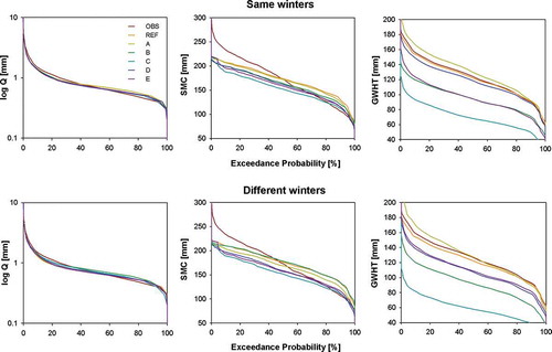
The daily patterns of soil moisture content with different interception losses are closely correlated to the observed values. The most satisfactory estimates were performed by models A, B and D, with overall differences in RMSE and the NSE coefficient up to 8% from the reference run (model A exhibited no deterioration in RMSE). The NSE reached 0.69 when model A was used, and in the case of models B and D, it was 0.64 and 0.63, respectively. In contrast, models C and E differed in RMSE by 20 and 12%, respectively, and their NSE coefficient was below 0.60. In general, all the models overestimated lower and underestimated higher soil moisture contents (Fig. 6).

When considering the daily groundwater levels, there were notable deviations between the observed and estimated values, even when comparing the reference run to the observations (Fig. 4). This resulted from model calibration with respect to discharge, which resulted in very low NSE values (up to 0.1). The most accurate models were models A and D (RMSE ~20 mm: an increase of up to 10% compared to the reference run). The worst result originated from model C, with an RMSE increase of more than 64% compared to the reference run (all other models were below this value). The probabilistic distribution of the groundwater levels output by models A and D was in close correspondence to the observed value distribution (Fig. 6).

In summary, model D exhibited the best results, with a satisfactory discharge simulation (RMSE increased by 3.4% compared to the reference run), a slightly biased soil moisture simulation (RMSE up by 7.8%) and a good groundwater level assessment (worsened by 0.7%). It was followed by models B (having less satisfactory groundwater storage [GWHT] estimation), A (slightly worse discharge RMSE) and then E (less satisfactory GWHT and soil moisture content [SMC] estimation). Model C did not perform well in terms of estimating the soil moisture (NSE < 0.55) or the groundwater level (increase in RMSE > 60%).

3.5 Water cycle modelling using estimated interception for the entire year

Modelling of the winter interception and the interception over the growing seasons demonstrated some minor changes in the prediction of discharge (Q), SMC and GWHT. In the case of discharge, models D and B reported improved results compared to the reference run, with the RMSE values decreasing by 1% and 3%, respectively. The improved results are due to the fact that these two models estimated a lower winter interception compared to the observed values obtained based on the regression equation (Šípek and Tesař 2014). The lower interception caused an increased precipitation amount, which was beneficial for the water balance (the difference in runoff volume was up to 2% on average using these interception models). This was documented by the decrease in the SFCF parameter (Table 4) compared to the other interception models, indicating that there was a sufficient amount of precipitation when the interception was underestimated. The NSE value ranged from 0.73 (model A) to 0.78 (model B). The probability distribution of the discharges was similar for all models (Fig. 6).

The use of modelled winter interception revealed that the least accurate soil moisture content estimation is in model C (NSE 0.51). The RMSE increased by, on average, 20%. The NSE coefficient of models B, D and E worsened to values closer to 0.60, and their RMSE values rose by 8–14% compared to the reference run. In contrast, model A did not show any worsening of the simulated soil moisture accuracy, even when the winter interception was estimated by the model (RMSE decreased by 1.0%). The major changes in the probability distribution curve were related to the two worst models, which tended to underestimate lower soil water contents more markedly.

The effect of the winter interception estimation on the model efficiency concerning groundwater level estimation was similar to that when interception was modelled only during the growing season. The reason for this is that the underestimated interception by models B, C and D (see section 3.2) was mitigated by the decreased SFCF parameter resulting from calibration (Table 4). The best results were obtained from models E, D and A, with RMSE increases of 18, 23 and 32%, respectively. Models B and C achieved RMSEs over 40% higher than those of the reference run.

As a result, model A achieved the highest accuracy, as the simulated discharge was satisfactory (NSE = 0.73), simulated soil moisture was improved compared to the reference run (RMSE improved by 1%), and simulated groundwater showed an RMSE increase of 32%. The second best was model B, despite having a notably worse groundwater simulation (RMSE up by 44%). The remaining models had deteriorated soil moisture simulations, as the RMSE increased more than 10% compared to the reference run.

3.6 Water balance

As the interception models differed in their estimated amount of interception loss, the water balance could be altered. The partition of actual evapotranspiration and the mean annual rates of its components are depicted in Table 5. The differences between the modelled and simulated rates of interception were presented above (section 3.2). As the HBV model was calibrated with respect to discharge, the differences in the modelled rates of mean annual actual evapotranspiration were relatively small (up to 4.8% from the reference run in the case of model D). The optimum results concerning the estimated annual AET were obtained from model C, followed by models E and A. The AET was overestimated by 0.5% (same winters) and underestimated by 0.8% (different winters) in the case of model C. The differences were up to 3% in the case of the two runner-up models (E and A). The similarity among the models resulted from the propensity of the calibration procedure to appropriately capture the total runoff volume, hence adjusting the rate of transpiration when the interception was underestimated/overestimated. As a result, the total AET was fairly stable, but its two fundamental components (evaporation and transpiration) varied more noticeably.

Table 5. Annual average water balance components from the HBV model in the period 2009–2018. VOLQ – change in runoff volume from observed values, TRANS – rate of transpiration, INT_S – interception in the growing season (May–October), INT_W – interception in winter and AET – rate of actual evapotranspiration. Δ denotes the percentage difference from the reference model run (REF)

	VOLQ	TRANS	INT_S	INT_W	AET	ΔTRANS	ΔINT	ΔAET
	%	mm	mm	mm	mm	%	%	%
REF	−1.9	325	135	121	581	-	-	-
Same winters
A	−2.7	326	141	121	588	0.3	2.3	1.2
B	−5.0	339	135	121	595	4.3	0.0	2.4
C	−6.4	287	177	121	585	−11.7	16.0	0.5
D	−5.7	343	138	121	602	5.7	1.2	3.7
E	−5.8	297	177	121	595	−8.5	16.3	2.5
Different winters
A	−6.8	332	141	125	598	2.2	3.5	2.8
B	−0.6	348	135	75	558	7.0	−18.3	−4.2
C	−3.9	296	177	105	578	−8.7	9.3	−0.8
D	−4.9	353	138	119	610	8.6	0.0	4.8
E	−8.2	294	177	120	591	−9.6	15.6	1.5

The smallest difference in mean annual transpiration (compared to the reference run) was reported by model A. In both modelling experiments, the annual sum of transpiration differed by 0.3% (interception estimated only in growing season) and by 2.2% (interception modelled year round) from the reference run. In the growing season, models B and D overestimated transpiration by 4.3% and 5.7%, respectively. The two remaining models underestimated transpiration by over 8%. In the case of different winter scenarios, the differences in mean annual transpiration were consistently over 7% on average for all models, excluding model A.

In terms of the correct evapotranspiration partitioning and the catchment water balance, model A exhibited the highest accuracy. It reasonably estimated the total AET (difference of less than 2.8%) as well as the separate rates of transpiration and interception (difference less than 3.5%). Altogether, all inspected models were sensitive to the value of interception loss when distinguishing the particular processes included in actual evapotranspiration. The influences on discharge, soil moisture and groundwater simulations were of lower a magnitude, as the model tended to compensate for the changing rate of interception by adjusting the rate of transpiration. Hence, for accurate hydrological simulation, information about seasonal interception rates is necessary.

4 Discussion

4.1 Measured interception

In general, the interception/gross precipitation (I/P_G) ratios were slightly lower than the results of other case studies performed in the Norway spruce forests. For example, Dohnal et al. (2014) found the interception to be approximately 33 and 36% at the same site in the growing seasons of 2012 and 2013, respectively. Similar results were presented by Ringgaard et al. (2014), who found the precipitation interception rate to be approximately 32–37% for the Norway spruce forests in western Denmark. Several older studies from the mountainous regions in the Czech Republic showed similar I/P_G ratios, ranging from 28 to 31% (Krečmer 1968, Krečmer and Fojt 1981). In contrast, Peng et al. (2014) analysed canopy interception in a Qinghai spruce forest in northwest China, where the total interception loss reached 73–93% (due to the high canopy storage capacity of the trees and loss from strong evaporation processes). The differences resulted from the different precipitation characteristics of the inspected years (Peng et al. 2014) and variations in the canopy structure (Pypker et al. 2005, Jeong et al. 2019). In this study, a 10-year period was investigated, and in some years, the same I/P_G ratios as found in other studies were observed.

The spatial variability of throughfall is one of the factors that has the potential to negatively influence the accuracy of the results. The four raingauges used in this study did not have to cover the entire variability of canopy structure; however, the positions of the raingauges cover a wide range of crown closure (ranging from 18 to 95%). The differences in the throughfall amounts, among the raingauges, varied up to 10% on a long-term basis. The recorded throughfall varied more within particular events. Studies focused on the description of the spatial variability of throughfall have discovered variability in tens of percentages for long-term averages (Holko et al. 2009, Dohnal et al. 2014) or even larger variations for at a scale of particular events (Keim et al. 2005). Moreover, the decline in the spatial variability of throughfall with forest thinning was noted, for example, by Vaca et al. (2018), which would on the contrary diminish the effect of a lower number of raingauges (as the forest is over 100 years old). However, it was assumed that the spatial variability did not notably deteriorate the results, as the I/P_G ratio corresponded to those reported in similar regions.

The estimated interception during the winter period can also be influenced by the spatial variability of the snow cover; however, several measurements (three at minimum) were always collected at the same time. Hence, the regression-based relationship used for the prediction of snow depth under forest canopies could have been a source of error. Additionally, as we have used this relationship (estimating the winter interception to be equal to 40.8%) for the prediction of throughfall in the winter period (November–April), it overestimated the interception in the cases when rainfall was observed (instead of snowfall). The average observed rate of rain interception was 29.1%; therefore, there was a 12% difference at maximum that could influence the throughfall estimation in the winter period in the reference model run and similar winter scenarios. However, if we consider the possibility of higher rainfall interception by the forest canopy covered by snow, then this difference should form the uppermost boundary, and the real boundary should be lower.

It is necessary to stress that the spatial variability of throughfall estimates (not completely covered by a limited number of raingauges) could deviate the comparison of interception estimates and interception model parameters from the values obtained in other studies benefiting from more reliable throughfall measurements (i.e. a larger number of raingauges or throughfall troughs). However, the presented measurements should be sufficient for the purpose of this study, as its main aim was not to publish a high-quality throughfall dataset. The study dealt primarily with a comparison of different interception models, with a focus on soil moisture, groundwater and runoff simulations. As the parameters of all interception models were derived from the same (possibly biased) throughfall dataset, then this possible bias was similar for all interception models. Hence, it did not influence their comparison.

4.2 Interception modelling

Interception modelling on a daily time scale is associated with several difficulties. Muzylo et al. (2009) stated that the volume error of interception loss models can be classified as follows: bad (> 30% of observed interception loss); fair (10% < error ≤ 30%); good (5% < error ≤ 10%); very good (1% < error ≤ 5%); or extremely good (error ≤ 1%). In these terms, models A and D were classified as very good, model B was classified as good, and models C and E were classified as bad (mean square error equalled 31% in both models).

The error of models C and E originated in the estimated model parameters. Model C is a version of model B (linear model without an intercept) that takes the long-term I/P_G ratio determined by Dohnal et al. (2014) as the constant relating I to P_G on a daily basis. This study confirmed that the I/P_G ratio was close to 30%. However, it was reported (in section 3.1) that the I/P_G ratio is dependent on the climate characteristics of the year; therefore, it was clearly not a suitable value for application to all rainfall events. The average value of in-storm evaporation E (0.44 mm/h) was generally higher than those reported by Gash et al. (1995) and Bryant et al. (2005). In contrast, the rate of E corresponded to those presented by Loustau et al. (1992) and Pypker et al. (2005). The values of the threshold necessary to saturate the canopy (P´_G) were within the range of 1.5–2.1 presented by Dohnal et al. (2014), Bryant et al. (2005) and Pypker et al. (2005) for conifer trees. The inefficiency of the Gash model (model E) was therefore produced not by implausible parameter values but more likely by application of the parameters derived from the limited number of events to all recorded rainfall events. The event-based regression analysis was restricted to the events occurring during the day that were preceded by successive rainless hours. However, a significant number of rainfall events in the experimental area occurred during the night or in rapid succession. As the independence of individual rainfall events is a primary assumption of the Gash model, the real in-storm evaporation may be lower (Gash 1979).

Additionally, Eliáš et al. (1995) described the influence of cloud water on the water balance in the area as constituting approximately 7–10% of the total precipitation, which lowers the actual rate of interception, as the canopy will often be saturated prior to the beginning of rainfall. If the values of E and P´_G are calibrated, then the Gash model will exhibit similar results to the remaining models (in terms of interception and hydrological simulations), but the derivation of its parameters would not be realistic. In this case, when we keep P´_G equal to 2.1 mm (this value seems to be more stable than E), E must be decreased to 0.17 mm/h. However, such a value was rarely observed in the inspected events. The trunk parameters were not inspected thoroughly, as the stemflow data were not available. Moreover, their decreased influence on the modelled amount of interception (compared to P´_G and E) was reported by Su et al. (2016).

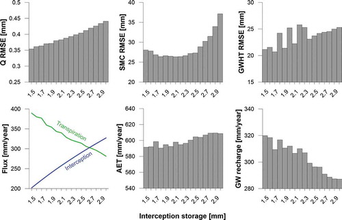
The key parameters of models A and E were represented by the interception capacity/threshold necessary to saturate the canopy and by in-storm evaporation. The sensitivity of these models to the changes in their values was tested by means of their variation within a plausible range (P´_G: 1.5–3.5 mm, E: 0.1–0.5 mm/h) and the repetitive calibration of the hydrological model according to the scheme described in section 2.4. First, the influence of changes in interception capacity was investigated using the threshold model (model A). The RMSE gradually rose from 0.35 to 0.45 mm in the case of discharge, and from 27 to 37 mm considering soil water content (although it was stable up to the interception capacity of 2.5 mm), and was nearly constant in the case of groundwater level (approximately 20–25 mm). The most important differences were shown in the water balance. In both investigated models, increasing the maximum interception capacity resulted in an increased amount of interception at the expense of transpiration (Fig. 7).

Figure 7. The influence of canopy storage on discharge (Q), soil moisture content (SMC), groundwater storage (GWHT), actual evapotranspiration (AET) and groundwater recharge (GW recharge) simulations using the threshold model (model A). The horizontal axis represents constantly changing canopy storage from 1.5 to 3.0 mm

Second, considering the Gash model (model E), the RMSE of the discharge estimation varied from 0.37 to 0.44 mm when the P´_G value was changed from 1.5 to 3.5 mm (E was fixed to 0.44 mm/h). The soil moisture RMSE ranged from 27 to 51 mm, and the error in groundwater level estimation decreased from 33 to 26 mm (with a minimum of 21 mm when P´_G was 2.5 mm). The resulting AET remained the same. Moreover, the Gash model included in-storm evaporation which also influenced RMSE values. The RMSE of the discharge estimation varied from 0.36 to 0.38 mm when in-storm evaporation was changed from 0.1 to 0.5 mm/h (P´_G was fixed to 2.1 mm). The soil moisture RMSE ranged from 28 to 31 mm, and the error in groundwater level estimation increased from 20 to 25 mm.

To summarize, all investigated variables were sensitive to the values of model parameters, with the groundwater level being the least affected. Additionally, the influence of canopy storage and the threshold necessary to saturate the canopy on resulting hydrological simulations was higher (based on changes in RMSE) compared to in-storm evaporation. This was evidenced by the fact that even small changes in P´_G influenced every single rainfall in terms of throughfall amount. Contrarily, the changes in in-storm evaporation affected only the rainfalls exceeding P´_G. Hence, interception capacity evenly affected all inspected variables (discharge, soil water and groundwater level). In contrast, the influence of different rates of in-storm evaporation was identified specifically during high water levels, as they specifically affect the rainfalls above the canopy storage threshold.

5 Conclusion

The study reports the influence of differently estimated interception in a mature spruce forest on the modelling of runoff, soil water and groundwater level. The annual average observed interception equalled 135 mm (29.1% of gross precipitation) during the growing season (May–October). The ratio of intercepted rainfall to gross rainfall was negatively correlated with both the number of rainfall events higher than 10 mm/d and the total rainfall amount.

The modelling experiments showed that even simple interception models (e.g. threshold or power models) can serve as a sufficient tool in hydrological simulations. The only requirement is that they need to reasonably estimate the overall rate of interception occurring during the inspected time period. The parameters for the most common Gash interception model were determined, but they were found to be insufficient for performing long-term interception estimations at the site, due to the frequent nonindependence of consecutive rainfall events and the influence of cloud water. Both factors contributed to the lowering of the real in-storm evaporation and threshold necessary to saturate the canopy.

It must be stressed that the key factor for accurate water balance estimation is the proper determination of the interception capacity or the precipitation multiplication coefficient. With this in mind, these simple models can be used efficiently instead of measuring throughfall in the spruce forests of Central Europe.

Disclosure statement

No potential conflict of interest was reported by the authors.

Additional information

Funding

This work was supported by the Czech Academy of Sciences [RVO 67985874]; Czech Science Foundation [GA CR 20-00788S]; Faculty of Science, Charles University in Prague [SVV 260438].

References

- Arnold, J.G., Allen, P.M., and Bernhardt, A., 1993. A comprehensive surface-groundwater flow model. Journal of Hydrology, 142, 47–69. doi:10.1016/0022-1694(93)90004-S
- Bergström, S., 1992. The HBV model: its structure and applications. Norrköping: Swedish Meteorological and Hydrological Institute (SMHI).
- Bryant, M., Bhata, S., and Jacobs, J., 2005. Measurements and modeling of throughfall variability for five forest communities in the southeastern US. Journal of Hydrology, 312, 95–108. doi:10.1016/j.jhydrol.2005.02.012
- Carlyle-Moses, D.E. and Gash, J.H.C., 2011. Rainfall interception loss by forest canopies. In: D.F. Levia, D. Carlyle-Moses, and T. Tanaka, eds. Forest hydrology and biogeochemistry. Heidelberg, Netherlands: Springer, 407–423.
- David, T.S., et al., 2006. Rainfall interception by an isolated evergreen oak tree in a Mediterranean savannah. Hydrological Processes, 20, 2713–2726. doi:10.1002/hyp.6062
- Dohnal, M., et al., 2014. Rainfall interception and spatial variability of throughfall in spruce stand. Journal of Hydrology and Hydromechanics, 62 (4), 277–284. doi:10.2478/johh-2014-0037.
- Eliáš, V., Tesař, M., and Buchtele, J., 1995. Occult precipitation: sampling, chemical analysis and process modelling in the Sumava Mts., (Czech Republic) and in the Taunus Mts. (Germany). Journal of Hydrology, 166, 409–420. doi:10.1016/0022-1694(94)05096-G
- Gash, J., Lloyd, C., and Lachaud, G., 1995. Estimating sparse forest rainfall interception with an analytical model. Journal of Hydrology, 170, 79–86. doi:10.1016/0022-1694(95)02697-N
- Gash, J.H.C., 1979. An analytical model of rainfall interception by forests. Quarterly Journal of the Royal Meteorological Society, 105, 43–55. doi:10.1002/qj.49710544304
- Gash, J.H.C. and Morton, A.J., 1978. An application of the Rutter model to the estimation of the interception loss from Thetford forest. Journal of Hydrology, 38, 49–58. doi:10.1016/0022-1694(78)90131-2
- Gerrits, A.M.J., et al., 2007. New technique to measure forest floor interception – an application in a beech forest in Luxembourg. Hydrology and Earth System Sciences, 11, 695–701. doi:10.5194/hess-11-695-2007
- Hadiwijaya, B., et al., 2020. The dynamics of transpiration to evapotranspiration ratio under wet and dry canopy conditions in a humid Boreal forest. Forests, 11, 237. doi:10.3390/f11020237
- Hlavinka, P., et al., 2011. Development and evaluation of the SoilClim model for water balance and soil climate estimates. Agricultural Water Management, 98, 1249–1261. doi:10.1016/j.agwat.2011.03.011
- Holko, L., et al., 2009. Impact of spruce forest on rainfall interception and seasonal snow cover evolution in the Western Tatra Mountains, Slovakia. Biologia, 64, 594–599. doi:10.2478/s11756-009-0087-6
- Jeníček, M. and Ledvinka, O., 2020. Importance of snowmelt contribution to seasonal runoff and summer low flows in Czechia. Hydrology and Earth System Sciences, 24, 3475–3491. doi:10.5194/hess-24-3475-2020
- Jeong, S., Otsuki, K., and Farahnak, M., 2019. Relationship between stand structures and rainfall partitioning in dense unmanaged Japanese cypress plantations. Journal of Agricultural Meteorology, 75 (2), 92–102. doi:10.2480/agrmet.D-18-00030.
- Keim, R.F., Skaugset, A.E., and Weiler, M., 2005. Temporal persistence of spatial patterns in throughfall. Journal of Hydrology, 314, 263–274. doi:10.1016/j.jhydrol.2005.03.021
- Kermavnar, J. and Vilhar, U., 2017. Canopy precipitation interception in urban forests in relation to stand structure. Urban Ecosystems, 20, 1373–1387. doi:10.1007/s11252-017-0689-7
- Kofroňová, J., Tesař, M., and Šípek, V., 2019. The influence of observed and modelled net longwave radiation on the rate of estimated potential evapotranspiration. Journal of Hydrology and Hydromechanics, 67 (3), 280–288. doi:10.2478/johh-2019-0011.
- Krečmer, V., 1968. K intercepci srážek ve středohorské smrčině (On the interception of spruce forest in mountainous regions). Opera Corcontica, 5, 83–96.
- Krečmer, V. and Fojt, V., 1981. Intercepce smrčin chlumní oblasti (Interception of conifer trees in middle altitudes). Vodohospodářský časopis, 1, 33–49.
- Larssen, T., Høgåsen, T., and Cosby, B.J., 2007. Impact of time series data on calibration and predictionuncertainty for a deterministic hydrogeochemical model. Ecological Modelling, 207, 22–33. doi:10.1016/j.ecolmodel.2007.03.016
- Li, X., et al., 2016. Process-based rainfall interception by small trees in Northern China: the effect of rainfall traits and crown structure characteristics. Agricultural and Forest Meteorology, 218–219, 65–73. doi:10.1016/j.agrformet.2015.11.017
- Linhoss, A.C. and Siegert, C.M., 2016. A comparison of five forest interception models using global sensitivity and uncertainty analysis. Journal of Hydrology, 538, 109–116. doi:10.1016/j.jhydrol.2016.04.011
- Liu, J., Zhang, Z., and Zhang, M., 2018. Impacts of forest structure on precipitation interception and run-off generation in a semiarid region in northern China. Hydrological Processes, 32, 2362–2376. doi:10.1002/hyp.13156
- Llorens, P. and Domingo, F., 2007. Rainfall partitioning by vegetation under Mediterranean conditions. A review of studies in Europe. Journal of Hydrology, 335, 37–54. doi:10.1016/j.jhydrol.2006.10.032
- Loustau, D., Berbigier, P., and Granier, A., 1992. Interception loss, throughfall and stemflow in a maritime pine stand. II. An application of Gash’s analytical model of interception. Journal of Hydrology, 138, 469–485. doi:10.1016/0022-1694(92)90131-E
- Magliano, P.N., Whitworth-Hulse, J.I., and Baldi, G., 2019. Interception, throughfall and stemflow partition in drylands: global synthesis and meta-analysis. Journal of Hydrology, 568, 638–645. doi:10.1016/j.jhydrol.2018.10.042
- Mauch, K.J., et al., 2008. New weighing method to measure shoot water interception. Journal of Irrigation and Drainage Engineering, 134 (3), 349–355. doi:10.1061/(ASCE)0733-9437(2008)134:3(349).
- Monteith, J.L., 1965. Evaporation and environment. Symposia of the Society for Experimental Biology, 19, 205–234.
- Moore, G., Bond, B.J., and Jones, J.A., 2011. A comparison of annual transpiration and productivity in monoculture and mixed-species Douglas-fir and red alder stands. Forest Ecology and Management, 262, 2263–2270. doi:10.1016/j.foreco.2011.08.018
- Muzylo, A., et al., 2009. A review of rainfall interception modelling. Journal of Hydrology, 370 (1–4), 191–206. doi:10.1016/j.jhydrol.2009.02.058.
- Nanko, K., Hotta, N., and Suzuki, M., 2006. Evaluating the influence of canopy species and meteorological factors on throughfall drop size distribution. Journal of Hydrology, 329, 422–431. doi:10.1016/j.jhydrol.2006.02.036
- Návar, J., 2020. Modeling rainfall interception loss components of forest. Journal of Hydrology, 584, 124449. doi:10.1016/j.jhydrol.2019.124449
- Pearce, A.J. and Rowe, L.K., 1981. Rainfall interception in a multistoried, evergreen mixed forest: estimates using Gash’s analytical model. Journal of Hydrology, 49, 341–353. doi:10.1016/S0022-1694(81)80018-2
- Peng, H., et al., 2014. Canopy interception by a spruce forest in the upper reach of Heihe River basin, Northwestern China. Hydrological Processes, 28, 1734–1741. doi:10.1002/hyp.9713
- Pypker, T.G., et al., 2005. The importance of canopy structure in controlling the interception loss of rainfall: examples from a young and an old-growth Douglas-fir forest. Agricultural and Forest Meteorology, 130, 113–129. doi:10.1016/j.agrformet.2005.03.003
- Ringgaard, R., Herbst, M., and Friborg, T., 2014. Partitioning forest evapotranspiration: interception evaporation and the impact of canopy structure, local and regional advection. Journal of Hydrology, 517, 677–690. doi:10.1016/j.jhydrol.2014.06.007
- Rutter, A.J., Morton, A.J., and Robins, P.C., 1975. A predictive model of rainfall interception in forest: II. Generalization of the model and comparison with observations in some coniferous and hardwood stands. Journal of Applied Ecology, 12 (1), 367–380. doi:10.2307/2401739.
- Savenije, H.H.G., 2004. The importance of interception and why we should delete the term evapotranspiration from our vocabulary. Hydrological Processes, 18, 1507–1511. doi:10.1002/hyp.5563
- Seibert, J., 1997. Estimation of parameter uncertainty in the HBV model. Nordic Hydrology, 28, 247–262. doi:10.2166/nh.1998.15
- Seibert, J., 2000. Multi-criteria calibration of a conceptual runoff model using a genetic algorithm. Hydrology and Earth System Sciences, 4, 215–224. doi:10.5194/hess-4-215-2000
- Seibert, J. and Vis, M., 2012. Teaching hydrological modeling with a user-friendly catchment-runoff-model software package. Hydrology and Earth System Sciences, 16, 3315–3325. doi:10.5194/hess-16-3315-2012
- Šípek, V. and Tesař, M., 2014. Seasonal snow accumulation in the mid-latitude forested catchment. Biologia, 69, 1562–1569. doi:10.2478/s11756-014-0468-3
- Šípek, V. and Tesař, M., 2016. Validation of a mesoscale hydrological model in a small-scale forested catchment. Hydrology Research, 47 (1), 27–41. doi:10.2166/nh.2015.220.
- Šípek, V. and Tesař, M., 2017. Year-round estimation of soil moisture content using temporally variable soil hydraulic parameters. Hydrological Processes, 31, 1438–1452. doi:10.1002/hyp.11121
- Staelens, J., et al., 2008. Rainfall partitioning into throughfall, stemflow, and interception within a single beech (Fagus sylvatica L.) canopy: influence of foliation, rain event characteristics, and meteorology. Hydrological Processes, 22, 33–45. doi:10.1002/hyp.6610
- Su, L., et al., 2016. Modelling interception loss using the revised Gash model: a case study in a mixed evergreen and deciduous broadleaved forest in China. Ecohydrology, 9, 1580–1589. doi:10.1002/eco.1749
- Tolasz, R., et al., 2007. Climate atlas of Czechia. Prague: Czech Hydrometeorological Institute, 256.
- Vaca, C.C., Ghimire, C.P., and Van der Tol, C., 2018. Spatial patterns and temporal stability of throughfall in a mature Douglas-fir forest. Water, 10 (3), 317.
- Van Stan, J.T., Van Stan, J.H., and Levia, D.F., 2014. Meteorological influences on stemflowgeneration across diameter size classes of two morphologically distinct deciduous species. International Journal of Biometeorology, 58, 2059–2069. doi:10.1007/s00484-014-0807-7
- Wang, D. and Wang, L., 2017. Dynamics of evapotranspiration partitioning for apple trees ofdifferent ages in a semiarid region of northwest China. Agricultural Water Management, 191, 1–15. doi:10.1016/j.agwat.2017.05.010
- Zabret, K., Rakovec, J., and Šraj, M., 2018. Influence of meteorological variables on rainfall partitioning for deciduous and coniferous tree species in urban area. Journal of Hydrology, 558, 29–41. doi:10.1016/j.jhydrol.2018.01.025
- Zhang, Z.S., et al., 2016. Gross rainfall amount and maximum rainfall intensity in 60-minute influence on interception loss of shrubs: a 10-year observation in the Tengger Desert. Scientific Reports, 6, 10.