The lumped Muskingum flood routing model revisited: the storage relationship

ABSTRACT

Muskingum models are a type of hydrological flood routing approach and vary only in the form of storage relationship. The storage relationship was first established based on the weighted arithmetic mean. The weighted arithmetic averaging used in the classical linear Muskingum models is not the only way to express the storage in the river reach. This study proposes a generalized Muskingum model by establishing the storage using the weighted power mean between the storage volumes due to the inflow and outflow. All traditional models are special cases of the proposed model. The proposed model reduces to four novel storage equations that have not been reported before. The results show the proposed models (a) effectively capture the characteristics of the flood wave, (b) lead to results with higher efficiency compared to the traditional Muskingum models and (c) make it possible to select the most efficient model for a given river.

KEYWORDS:

• weighted power mean
• storage equations
• flood routing
• river reach

Editor A. Castellarin Associate Editor B. Dewals

1 Introduction

Flood routing plays an important role in calculating the shape of flood waves along river reaches. Hydraulic and hydrological methods are two widely used flood routing approaches. Although both approaches use the principle of conservation of mass (via a one-dimensional continuity equation), the hydraulic approach considers flow dynamic effects using the momentum equation, while the hydrological approach does not and simply uses the storage equation without considering variable backwater effects such as downstream hydraulic structures (Barati et al. 2012, 2013). The accuracy of hydrological methods may be less than that of hydraulic methods but their application is much easier and more cost-effective.

The Muskingum model is a popular hydrological method that has been extensively applied in river engineering practice and used in numerous aggregated rainfall–runoff models. The Muskingum method (first developed by McCarthy in 1938 in the Muskingum River basin, Ohio) is a semi-theoretical model for flood routing in rivers and channels. This linear Muskingum model is easy to use and requires only the assessment of two empirical parameters (Karahan et al. 2013). However, this model may not be able to simulate the flood process accurately (Yoon and Padmanabhan 1993) since the discharge–storage relationship of the problem is usually nonlinear (Beven 2011). The Muskingum model provides a practical approach especially for unmanaged catchments for which the required data (on cross-sections, morphology, river bed slopes and roughness coefficients) are not available for the simulation of flood events via the full Saint Venant system of partial differential equations (Barati 2013). The application of the Muskingum model involves the calibration (optimization) and prediction (simulation) steps. In both steps a suitable numerical solution method for solving the governing equations is required (Vatankhah 2014a). The calibration step involves optimizing the model parameters using a set of inflow–outflow hydrographs. In the simulation step, a routing problem is numerically solved in which the outflow hydrograph is determined for a given inflow hydrograph. The Muskingum model parameters can be determined for a channel reach if observed inflow–outflow hydrographs are available for a flood event. Then, the model parameters are assumed to remain constant for other flood events (Akan 2006).

All existing Muskingum models use the theoretical continuity equation, but they use different empirical storage equations. Muskingum models are often classified based on their empirical storage equation into (a) classical linear Muskingum model and (b) nonlinear Muskingum models. Linear models are often used in hydrology modelling due to their simplicity and low cost; however, almost all physical hydrological systems are nonlinear. Most often, researchers have focused on improving the Muskingum model performance in the calibration step using new optimization algorithms and different optimization approaches (Mohan 1997, Kim et al. 2001, Geem 2006, 2011, Chu and Chang 2009, Luo and Xie 2010, Xu et al. 2012). But these efforts have resulted in little success (Easa 2014a). This study focuses on generalizing the Muskingum model structure, instead of applying optimization algorithms that produce only slight improvements in most cases.

The storage equation in the original Muskingum model is linear. To account for the nonlinearity of flood waves and to improve the performance of the original Muskingum model, structurally modified Muskingum models have been proposed in the literature. The first nonlinear storage equation of the Muskingum model was derived and proved by Chow (1959). This storage equation is not popular for flood routing procedures (Gill 1978). The most widely used nonlinear Muskingum model was proposed by Gill (1978) in an ad hoc manner and without any derivation or proof. After Gill’s nonlinear model, various studies have been conducted to consider the nonlinearity in flood routing problems. Most of these studies directly use Gill’s nonlinear storage equation. Several researchers have proposed new nonlinear variable-parameter Muskingum models with different structures for better accuracy (Easa 2013, 2014a, 2015a, 2015b, Karahan 2014, Vatankhah 2014b, Ayvaz and Gurarslan 2017, Niazkar and Afzali 2017, Bazargan and Norouzi 2018, Akbari et al. 2020). The Muskingum model should be calibrated using a set of inflow–outflow hydrograph data. By increasing the number of calibration parameters in the model, the data dependency of the model increases and the prediction power of the model may decrease; therefore, this research focuses on the nonlinear forms of the Muskingum model with the minimum number of model parameters.

Due to the nonlinear nature of flood wave movement in rivers, any effort to develop a general storage equation using basic principles of mathematics and hydraulics would be of practical importance. Unlike the previous studies that have mainly focused on improving the optimization algorithms (with little success), or focused on the variable-parameter Muskingum models and partitioning the inflow hydrograph into a finite number of sub-regions (with high data dependency), this study focuses on developing the storage equation of the Muskingum model in a general nonlinear form. The classical Muskingum model is based on the weighted arithmetic mean of storage volumes due to the inflow and outflow rates of a prismatic river reach. Since the weighted power mean is a generalized mathematical mean, this study proposes a general nonlinear Muskingum model with constant parameters by establishing the storage equation using the weighted power mean between the storage volumes due to the inflow and outflow rates.

2 Existing Muskingum models with constant calibration parameters

The theoretical continuity equation in differential form used in the flood routing Muskingum model is expressed as follows (Chow 1959):

(1) $\frac{dS}{dt}=I-O$(1)

where S, I, and O are, respectively, the volume of water storage in the channel reach [L³], upstream inflow discharge [L³T⁻¹] and downstream outflow discharge [L³T⁻¹] at time t. Equation (1)(1) $\frac{dS}{dt}=I-O$(1) is a lumped form of the mass conservation law.

The continuity equation should be solved simultaneously with a storage equation for hydrological flood routing. The empirical storage equation is a conceptual equation that is a replacement for the momentum equation, and is generally referred to as the Muskingum model. Different forms of the storage equation have been proposed in the literature. The relationship between weighted inflow and outflow discharges and storage is generally nonlinear. Thus, using the linear storage form [S = XI + (1 − X)O with X and K as constant numerical coefficients] may introduce considerable errors (Yoon and Padmanabhan 1993, Geem 2006).

The first nonlinear storage equation with an exponent parameter n associated with the inflow and outflow discharges was derived by Chow (1959) as the following:

(2) $S=K\left[X{I}^n+\left(1-X\right)O^n\right]$(2)

in which n is a dimensionless parameter that accounts for the nonlinearity of flood wave behaviour; X is the dimensionless weighting parameter; and K is the storage coefficient for the river or channel reach, which has a dimension of [L³⁽¹⁻ⁿ⁾Tⁿ]. This nonlinear form is derived using representations of storage and discharge in the river reach as power functions of the average depth. Equation (2)(2) $S=K\left[X{I}^n+\left(1-X\right)O^n\right]$(2) is not common in flood routing modelling (Gill 1978). The classical linear model is obtained by assuming n = 1. In this case, the storage parameter K has dimension [T] and may have a value close to the travel time of flood peaks that move through the river reach. Sometimes, for prismatic channels, K is interpreted as the travel time of a flood wave in the classical linear model. The classical linear Muskingum model assumes a linear relationship between S, I and O, in place of the momentum equation.

Another storage equation is suggested by Gill (1978) as:

(3) $S=K[XI+\left(1-X\right)O{]}^m$(3)

where the exponent m is a dimensionless parameter that accounts for the nonlinearity of the flood wave; X is the dimensionless weighting parameter; and K is the storage parameter for the river reach, which has dimension of [L^3(1−m)T^m]. Gill (1978) added the exponent parameter m to the classical linear form of storage equation in an ad hoc manner (without any derivation) to account for the nonlinearity of the flood wave. Equation (3)(3) $S=K[XI+\left(1-X\right)O{]}^m$(3) is the most popular nonlinear storage equation with constant parameters.

Easa (2014b), in an ad hoc manner and without any derivation or proof, combined the nonlinear storage Equations (2)(2) $S=K\left[X{I}^n+\left(1-X\right)O^n\right]$(2) and (3(3) $S=K[XI+\left(1-X\right)O{]}^m$(3) ) as the following:

(4) $S=K[X{I}^n+\left(1-X\right)O^n{]}^m$(4)

So far, no basic proof has been provided for this nonlinear form.

In storage Equation (4)(4) $S=K[X{I}^n+\left(1-X\right)O^n{]}^m$(4) , an additional flow parameter, m, is added compared with storage Equation (2)(2) $S=K\left[X{I}^n+\left(1-X\right)O^n\right]$(2) . In this equation K has dimension of [L^3(1−nm)T^nm], in which n and m are dimensionless parameters. Generally, the storage model coefficients (n, m, X and K) are treated as calibration parameters into which the channel reach characteristics are lumped.

Another research effort in this area was presenting a new five-parameter nonlinear storage equation (Barati et al. 2014, Vatankhah 2014c, Vatankhah 2015a, 2015b) as follows:

(5) $S=K[X{I}^{n_1}+\left(1-X\right)O^{n_2}{]}^m$(5)

This model is obtained by combining Gill’s and Gavilan and Houck’s nonlinear models in an ad hoc manner. The storage Equation (5)(5) $S=K[X{I}^{n_1}+\left(1-X\right)O^{n_2}{]}^m$(5) has a nonlinear form but is not dimensionally homogeneous when n₁ ≠ n₂. For m = 1, this equation reduces to the proposed nonlinear model by Gavilan and Houck (1985) with different exponent parameters for the inflow and outflow discharges n₁ ≠ n₂. For m = 1 and n₁ = n₂ = n, this equation reduces to the nonlinear Equation (2)(2) $S=K\left[X{I}^n+\left(1-X\right)O^n\right]$(2) . For n₁ = n₂ = 1, this equation reduces to the nonlinear model proposed by Gill (1978), and for n₁ = n₂ = n, the proposed equation reduces to the nonlinear model proposed by Easa (2014b).

3 New general storage equation

The storage in a natural river reach depends on the inflow and outflow discharges and the geometric characteristics of the river reach (Akbari and Barati 2012). The derivation procedure for Equation (2)(2) $S=K\left[X{I}^n+\left(1-X\right)O^n\right]$(2) presented by Chow (1959) serves as the basis to develop other storage equations. Assuming that the flow discharge and storage characteristics at the upstream and downstream sections have the same functional form (I = ay^b, O = ay^b, S_in = cy^d and S_out = cy^d where y is the flow depth, a and b reflect the discharge-stage characteristics and c, d reflect the storage-stage characteristics of the reach), the storage due to inflow S_in and the storage due to outflow S_out in a prismatic river reach can be expressed as:

(6) $S_{in}=K{I}^n$(6)

(7) $S_{out}=O^n$(7)

in which n is a dimensionless flow parameter and K is the storage parameter for the river or channel reach and has dimension of [L³⁽¹⁻ⁿ⁾Tⁿ].

In Equations (6)(6) $S_{in}=K{I}^n$(6) and (7(7) $S_{out}=O^n$(7) ), the flow and storage characteristics at the upstream and downstream cross-sections of the river reach are considered similar. When this assumption is not established, the storage due to inflow S_in and storage due to outflow S_out can be expressed as follows (Barati et al. 2014):

(8) $S_{in}=K_1{I}^{n1}$(8)

(9) $S_{out}=K_2{O}^{n2}$(9)

where n1 and n2 are dimensionless flow parameters and K₁ and K₂ are storage parameters for the river reach, which have dimensions of [L^3(1−n1)Tⁿ¹] and [L^3(1−n2)Tⁿ²], respectively, for the case of n1 ≠ n2. Equations (8)(8) $S_{in}=K_1{I}^{n1}$(8) and (9(9) $S_{out}=K_2{O}^{n2}$(9) ) have four parameters, which may increase the data dependency of the model. For simplicity and to decrease the data dependency of the model, Equations (6)(6) $S_{in}=K{I}^n$(6) and (7(7) $S_{out}=O^n$(7) ) are considered with only two parameters in this research.

In this study, the storage in the channel or river reach is expressed using the weighted power mean (of order p ≠ 0, Qi et al. 2000) of S_in and S_out, as:

(10) $S=[X(S_{in}{)}^p+\left(1-X\right)(S_{out}{)}^p{]}^{\frac{1}{p}}$(10)

in which p ≠ 0 is the exponent parameter and X is the dimensionless weighting parameter assigned to express the relative importance of the inflow and outflow storages. When X approaches 0, the storage of the reach approaches S_out, and when X approaches 1, the storage of the reach approaches S_in. Both X and p are dimensionless parameters, and Equation (10)(10) $S=[X(S_{in}{)}^p+\left(1-X\right)(S_{out}{)}^p{]}^{\frac{1}{p}}$(10) is dimensionally homogeneous.

Substituting S_in and S_out from Equations (6)(6) $S_{in}=K{I}^n$(6) and (7(7) $S_{out}=O^n$(7) ) into (10), the general form of the storage equation can be expressed as

(11) $S=K[X{I}^{np}+\left(1-X\right)O^{np}{]}^{\frac{1}{p}}$(11)

in which K is the storage parameter for the river reach and has a dimension of [L³⁽¹⁻ⁿ⁾Tⁿ]. A valid equation or formula in physics must be homogeneous. This storage equation, with four constant parameters, is dimensionally homogeneous. The general storage Equation (11)(11) $S=K[X{I}^{np}+\left(1-X\right)O^{np}{]}^{\frac{1}{p}}$(11) has a clear mathematical concept based on the weighted power mean of order p of the storage due to inflow S_in and the storage due to outflow S_out. There is no such concept in Equation (4)(4) $S=K[X{I}^n+\left(1-X\right)O^n{]}^m$(4) with four constant parameters, which was obtained in an ad hoc manner. It is worth noting that, substituting S_in = KIⁿ and S_out = KOⁿ into S = K^1−m[XS_in + (1 − X)S_out]^m yields Equation (4)(4) $S=K[X{I}^n+\left(1-X\right)O^n{]}^m$(4) , thus Equation (4)(4) $S=K[X{I}^n+\left(1-X\right)O^n{]}^m$(4) is based on the power relation (ax^b) of the weighted arithmetic mean of S_in and S_out [XS_in + (1 − X)S_out]. Equation (4)(4) $S=K[X{I}^n+\left(1-X\right)O^n{]}^m$(4) is not as efficient as Equation (11)(11) $S=K[X{I}^{np}+\left(1-X\right)O^{np}{]}^{\frac{1}{p}}$(11) . The general mathematically based form of Equation (11)(11) $S=K[X{I}^{np}+\left(1-X\right)O^{np}{]}^{\frac{1}{p}}$(11) makes possible the derivation of some new and efficient nonlinear storage equations, as will be shown in the next few sections.

It is worth noting that Bozorg-Haddad et al. (2019) considered the interdependence of S_in at the ith and (i + 1)th time intervals to construct a new storage equation with eight parameters (and thus high data dependency). In the study of Bozorg-Haddad et al. (2019), S_in is considered as the weighted arithmetic mean of S_in,i and S_in,i+1, but S_out is not considered as the weighted arithmetic mean of S_out,i and S_out,i+1. This apparent inconsistency needs further investigation and clarifications.

3.1 Special forms of the general storage equation

General storage Equation (11)(11) $S=K[X{I}^{np}+\left(1-X\right)O^{np}{]}^{\frac{1}{p}}$(11) along with the continuity equation can be used for the Muskingum flood-routing models. This study focuses on the Muskingum models with low data dependency with a minimum number of parameters (two or three). The special cases of the general Equation (11)(11) $S=K[X{I}^{np}+\left(1-X\right)O^{np}{]}^{\frac{1}{p}}$(11) are presented in the following.

3.1.1 Special case of p = 1 (weighted arithmetic mean of S_in and S_out)

For p = 1, Equation (11)(11) $S=K[X{I}^{np}+\left(1-X\right)O^{np}{]}^{\frac{1}{p}}$(11) reduces to the nonlinear Equation (2).

3.1.2 Special case of p = 1/n

For p = 1/n, Equation (11)(11) $S=K[X{I}^{np}+\left(1-X\right)O^{np}{]}^{\frac{1}{p}}$(11) reduces to the nonlinear Equation (3)(3) $S=K[XI+\left(1-X\right)O{]}^m$(3) , proposed by Gill (1978).

3.1.3 Special case of p = −1 (weighted harmonic mean of S_in and S_out)

For p = −1, the general storage equation takes the form

(12) $S=K[X{I}^{-n}+\left(1-X\right)O^{-n}{]}^{-1}$(12)

in which K is the storage parameter for the river reach and has dimension of [L³⁽¹⁻ⁿ⁾Tⁿ]. This new form of the storage equation has not been derived before. For n = 1, this equation takes the form S = K[XI⁻¹ + (1 − X)O⁻¹]⁻¹ = K/[X/I+(1 − X)/O] with only two parameters, which was not reported in any previous studies. In this harmonic form, the storage parameter K has a dimension of [T]. This may be related to the wave travel time and may be important from a hydrodynamic point of view. In terms of the number of model parameters, this nonlinear form is comparable with the classical linear form of the storage equation with only two parameters (n = p = 1); that is, S = K[XI + (1 − X)O].

3.1.4 Special case of p→0 (weighted geometric mean of S_in and S_out)

When p approaches 0, the behaviour of the general storage Equation (11)(11) $S=K[X{I}^{np}+\left(1-X\right)O^{np}{]}^{\frac{1}{p}}$(11) is very important. In this case, the term S/K takes the indeterminate form 1^∞. This limit can be computed using L’Hopital’s rule (see the Appendix). The general storage equation when p→0⁺ takes the form

(13) $S=\underset{p\to 0^{+}}{lim}\left\{K{[X{I}^{np}+\left(1-X\right)O^{np}]}^{\frac{1}{p}}\right\}=K{I}^{nX}{O}^{n\left(1-X\right)}$(13)

in which K is the storage parameter for the river reach, with a dimension of [L³⁽¹⁻ⁿ⁾Tⁿ]. This new form of the storage equation is known as the weighted geometric mean. The weighted geometric mean is a well-known property of the power mean and is equal to the exponential of the weighted arithmetic mean of the natural logarithms of S_in and S_out [lnS = Xln(S_in) + (1 − X)ln(S_out)].

The weighted geometric mean storage lies between the weighted harmonic mean storage and the weighted arithmetic mean storage – that is, K[XI⁻ⁿ + (1 − X)O⁻ⁿ]⁻¹≤ KI^nXO^n(1−X)≤ K[XIⁿ + (1 − X)Oⁿ].

3.1.5 Special case of n = 1 and p→0

In the case of n = 1 and p→0, the general storage equation becomes

(14) $S=\underset{p\to 0^{+}}{lim}\left\{K{[X{I}^p+\left(1-X\right)O^p]}^{\frac{1}{p}}\right\}=K{I}^X{O}^{\left(1-X\right)}$(14)

which is a well-known property of the power mean. This is a new nonlinear form of the storage equation with only two parameters. In this geometric form, the storage parameter K has dimension [T]. This may be related to the wave travel time. This nonlinear two-parameter form is comparable with the classical linear form of the storage equation S = K[XI + (1 − X)O] and the new nonlinear two-parameter form obtained in this study as S = K[XI⁻¹ + (1 − X)O⁻¹]⁻¹. For these two-parameter models, K has a dimension of [T], and one obtains K[XI⁻¹ + (1 − X)O⁻¹]⁻¹ ≤ KI^XO^(1−X) ≤ K[XI + (1 − X)O].

3.1.6 Special case of n = 1 (weighted power mean of I and O)

In the case of n = 1 (weighted power mean of I and O), the general storage equation becomes

(15) $S=K[X{I}^p+\left(1-X\right)O^p{]}^{\frac{1}{p}}$(15)

This is a new nonlinear form of the storage equation with three parameters. In this nonlinear form, the storage parameter K has a dimension of [T]. This may be important from the hydrodynamic point of view.

A summary of the storage equations of the Muskingum model is given in Table 1. All equations (models) have been derived from the general storage Equation (11)(11) $S=K[X{I}^{np}+\left(1-X\right)O^{np}{]}^{\frac{1}{p}}$(11) which is based on the weighted power mean of S_in and S_out. Storage models 1–3 have two parameters and storage models 4–7 have three parameters. The novel storage models 1, 3, 6 and 7 are developed in this study, for the first time. Storage models 3 and 7 are based on the weighted geometric mean and can be represented in a general form as S = KI^nXO^n(1−X). The other models can be represented in a general form as S = K[XIⁿ + (1 − X)Oⁿ]^m.

Table 1. Summary of storage equations (special cases of the proposed general storage Equation (11))

Model	Special case	Resulting storage equation	Number of parameters
1	p = −1 n = 1	S = K[XI^−1 + (1 − X)O^−1]^−1	2
2	p = 1 n = 1	S = K[XI + (1 − X)O]	2
3	p→0 n = 1	S = KI^XO^(1−^X^)	2
4	p = 1	S = K[XI^n + (1 − X)O^n]	3
5	p = 1/n	S = K[XI + (1 − X)O]^m	3
6	p = −1	S = K[XI^−^n + (1 − X)O^−^n]^−1	3
7*	p→0	S = KI^nXO^n(1−X)	3
8	n = 1	S = K[XI^p + (1 − X)O^p]^1/p	3

*When storage characteristics at the upstream and downstream cross-sections of the river reach are different, using the limit property of the power mean, this storage equation takes the form S = KI^nXO^m(1−X). This model has one additional parameter m relative to model 3.

Models with the same number of parameters have the same degree of freedom and are comparable. The performance of the classical linear Muskingum model 2 (with two parameters) is comparable with the performance of the proposed nonlinear models 1 and 3. The performance of the nonlinear models 4 and 5 will be comparable with the performance of the proposed three-parameter nonlinear models 6, 7 and 8. According to three sets of flood data (three case studies) considered in this study, model 7 tends to approach model 3 (p tends to approach 0).

4 Muskingum models with lateral flows

In some situations, lateral flows may be observed along the river reach. In these cases, the volume of the outflow hydrograph will be different from the volume of the inflow hydrograph. The revised linear Muskingum model with lateral flow was first presented by O’Donnell (1985). Indicating the lateral flow as a ratio of the inflow rate, αI (Karahan 2014, Karahan et al. 2015), the revised version of the Muskingum model can be obtained by replacing I in the governing equation with I(1 + α) instead, as follows:

(16) $\frac{dS}{dt}=I\left(1+\alpha \right)-O$(16)

(17) $S=K[X(1+\alpha {)}^{np}{I}^{np}+\left(1-X\right)O^{np}{]}^{\frac{1}{p}}$(17)

in which α is a dimensionless parameter with a clear physical meaning. The lateral flow parameter, α, is positive for the lateral inflow and is negative for the lateral outflow. Lateral flows have no importance when α = 0. The need to apply α can be recognized by field observations, or by comparing the observed inflow and outflow hydrograph volumes used in the calibration phase. Vatankhah (2017) defined the volume ratio, r, as the ratio of the volume of the outflow hydrograph to the volume of the inflow hydrograph. The lateral flows will be in the river reach when r ≠ 1 (lateral inflow for r > 1 (α > 0) and lateral outflow for r < 1 (α < 0)).

Storage model 7, by incorporating the lateral flow, is expressed as:

(18) $S=K{ }^{\mathrm{\prime }}{I}^{nX}{O}^{n\left(1-X\right)}$(18)

in which K^׳  = K(1 + α)^nX. When lateral flows have no importance, K^׳  = K.

By incorporating the lateral flow effect, other storage models (models 1, 2, 4, 5, 6 and 8) can be expressed in a general form as:

(19) $S=K[X(1+\alpha {)}^n{I}^n+\left(1-X\right)O^n{]}^m$(19)

As shown, incorporating the lateral flow effects adds one more parameter to the storage models in the form of Equation (19)(19) $S=K[X(1+\alpha {)}^n{I}^n+\left(1-X\right)O^n{]}^m$(19) . In the case of no lateral flow (α = 0), general storage Equations (18)(18) $S=K{ }^{\mathrm{\prime }}{I}^{nX}{O}^{n\left(1-X\right)}$(18) and (19(19) $S=K[X(1+\alpha {)}^n{I}^n+\left(1-X\right)O^n{]}^m$(19) ) will reduce to the storage models of Table 1.

5 Routing and solving procedure

Explicit numerical solution methods have often been used in the literature for solving the Muskingum models. Since the simulation procedure is also a base for the optimization procedure, an accurate solution method such as the fourth-order Runge-Kutta method (Vatankhah 2010, 2014a, 2014b, 2014c, Easa 2015a, Vatankhah 2015a, 2015b, 2017, 2018) should be used to solve the Muskingum models. The accuracy of a numerical solution method depends on how close the discretized equation is to the original differential equation (Vatankhah 2017). Utilizing higher order solution methods must be balanced against their complexity. Through a comparison of different explicit methods, Vatankhah (2014a) showed that the explicit fourth-order Runge-Kutta method is a simple yet accurate solution method for solving the Muskingum model. The solution method used in this study is based on the fourth-order Runge-Kutta method, which is the most accurate and widely used numerical method for solving the initial value problems. This solution procedure is outlined in the following.

Nonlinear storage models 3 and 7 (Table 1) developed in this study for Muskingum flood routing can be combined in a unified model as Equation (18)(18) $S=K{ }^{\mathrm{\prime }}{I}^{nX}{O}^{n\left(1-X\right)}$(18) . Other models (models 1, 2, 4, 5, 6 and 8) can also be expressed as Equation (19)(19) $S=K[X(1+\alpha {)}^n{I}^n+\left(1-X\right)O^n{]}^m$(19) .

Solving Equation (18)(18) $S=K{ }^{\mathrm{\prime }}{I}^{nX}{O}^{n\left(1-X\right)}$(18) for O, the outflow is expressed as

(20) $O={\left[\frac{S}{K{ }^{\mathrm{\prime }}{I}^{nX}}\right]}^{\frac{1}{n\left(1-X\right)}}$(20)

Substituting O from Equations (20)(20) $O={\left[\frac{S}{K{ }^{\mathrm{\prime }}{I}^{nX}}\right]}^{\frac{1}{n\left(1-X\right)}}$(20) into (16), the storage rate can be expressed as

(21) $\frac{dS}{dt}=\left(1+\alpha \right)I-{\left[\frac{S}{K{ }^{\mathrm{\prime }}{I}^{nX}}\right]}^{\frac{1}{n\left(1-X\right)}}$(21)

For specified values of I, and the parameter values K^׳, X, α and n, Equation (21)(21) $\frac{dS}{dt}=\left(1+\alpha \right)I-{\left[\frac{S}{K{ }^{\mathrm{\prime }}{I}^{nX}}\right]}^{\frac{1}{n\left(1-X\right)}}$(21) forms a first-order ordinary differential equation.

Similarly, solving Equation (19)(19) $S=K[X(1+\alpha {)}^n{I}^n+\left(1-X\right)O^n{]}^m$(19) for O, the outflow can be expressed as

(22) $O={\left[\frac{{\left(\frac{S}{K}\right)}^{\frac{1}{m}}-X{(1+\alpha )}^n{I}^n}{1-X}\right]}^{\frac{1}{n}}$(22)

Substituting O from Equations (22)(22) $O={\left[\frac{{\left(\frac{S}{K}\right)}^{\frac{1}{m}}-X{(1+\alpha )}^n{I}^n}{1-X}\right]}^{\frac{1}{n}}$(22) into (16), the storage rate can be expressed as

(23) $\frac{dS}{dt}=\left(1+\alpha \right)I-{\left[\frac{{\left(\frac{S}{K}\right)}^{\frac{1}{m}}-X{(1+\alpha )}^n{I}^n}{1-X}\right]}^{\frac{1}{n}}$(23)

For specified values of I, and the parameter values K, X, α, n and m, Equation (23)(23) $\frac{dS}{dt}=\left(1+\alpha \right)I-{\left[\frac{{\left(\frac{S}{K}\right)}^{\frac{1}{m}}-X{(1+\alpha )}^n{I}^n}{1-X}\right]}^{\frac{1}{n}}$(23) forms a first-order ordinary differential equation.

Assume that the number of time intervals of the observed inflow hydrograph is denoted by N (number of nodes = N + 1). Then, the inflow, outflow and accumulated storage volume for time interval i are, respectively, denoted by I_i, O_i and S_i, where i = 0, 1, …, N. For i = 0, the initial values of inflow, outflow and accumulated storage volume are, respectively, denoted by I₀, O₀ and S₀.

5.1 Solution procedure for the general form of S = K^׳I^nXO^n(1−X)

The solution procedure using the fourth-order Runge-Kutta method for the general storage Equation (18)(18) $S=K{ }^{\mathrm{\prime }}{I}^{nX}{O}^{n\left(1-X\right)}$(18) is the following:

Step 1. Assume values for the model parameters K^׳, X, α and n [K^׳ = K(1 + α)^nX].

Step 2. Calculate the initial accumulated storage volume for i = 0 using the following equation:

(24) $S_i=K{ }^{\mathrm{\prime }}{I}_i^{nX}{O}_i^{n\left(1-X\right)}$(24)

where the initial computed outflow, O₀, is assumed to be equal to the initial observed inflow, I₀.

Step 3. Calculate the next accumulated storage, S_i+1, using the present value, S_i, plus the product of the size of the interval, Δt, and a weighted average storage rate as the following:

(25) $S_{i+1}=S_i+\mathrm{\Delta }t\frac{\left(a_i+2b_i+2c_i+d_i\right)}{6}$(25)

in which the storage rates a_i, b_i, c_i and d_i are:

(26) $\begin{array}{rl}& a_i=(1+\alpha )I_i-{\left[\frac{S_i}{K^{\prime }{I}_i^{nX}}\right]}^{\frac{1}{n(1-X)}}\\ & b_i=(1+\alpha )\left(\frac{I_i+I_{i+1}}{2}\right)-{\left[\frac{S_i+0.5a_i\mathrm{\Delta }t}{K^{\prime }{\left(\frac{I_i+I_{i+1}}{2}\right)}^{nX}}\right]}^{\frac{1}{n(1-X)}}\\ & c_i=(1+\alpha )\left(\frac{I_i+I_{i+1}}{2}\right)-{\left[\frac{S_i+0.5b_i\mathrm{\Delta }t}{K^{\prime }{\left(\frac{I_i+I_{i+1}}{2}\right)}^{nX}}\right]}^{\frac{1}{n(1-X)}}\\ & d_i=(1+\alpha )I_{i+1}-{\left[\frac{S_i+c_i\mathrm{\Delta }t}{K^{\prime }{I}_{i+1}^{nX}}\right]}^{\frac{1}{n(1-X)}}\end{array}$(26)

Step 4. Calculate the next outflow using the following equation:

(27) $O_{i+1}={\left[\frac{S_{i+1}}{K{ }^{\mathrm{\prime }}{I}_{i+1}^{nX}}\right]}^{\frac{1}{n\left(1-X\right)}}$(27)

Step 5. Repeat steps 3 and 4 for the subsequent time intervals.

5.2 Solution procedure for the general form of S = K[X(1 + α)ⁿIⁿ + (1− X)Oⁿ]^m

The solution procedure using the fourth-order Runge-Kutta method for the general storage Equation (19)(19) $S=K[X(1+\alpha {)}^n{I}^n+\left(1-X\right)O^n{]}^m$(19) is the following:

Step 1. Assume values for the model parameters K, X, α, n and m.

Step 2. Calculate the initial accumulated storage volume for i = 0 using the following equation:

(28) $S_i=K[X(1+\alpha {)}^n{I}_i^n+\left(1-X\right)O_i^n{]}^m$(28)

where the initial computed outflow, O₀, is assumed to be equal to the initial observed inflow, I₀.

Step 3. Calculate the next accumulated storage, S_i+1, using the present value, S_i, plus the product of the size of the interval, Δt, and a weighted average slope as the following:

(29) $S_{i+1}=S_i+\mathrm{\Delta }t\frac{\left(a_i+2b_i+2c_i+d_i\right)}{6}$(29)

in which the storage rates a_i, b_i, c_i and d_i are:

(30) $\begin{array}{rl}& a_i=(1+\alpha )I_i-{\left[\frac{{\left(\frac{S_i}{K}\right)}^{\frac{1}{m}}-X{(1+\alpha )}^n{I}_i^n}{1-X}\right]}^{\frac{1}{n}}\\ & b_i=(1+\alpha )\left(\frac{I_i+I_{i+1}}{2}\right)-{\left[\frac{{\left(\frac{S_i+0.5a_i\mathrm{\Delta }t}{K}\right)}^{\frac{1}{m}}-X{(1+\alpha )}^n{\left(\frac{I_i+I_{i+1}}{2}\right)}^n}{1-X}\right]}^{\frac{1}{n}}\\ & c_i=(1+\alpha )\left(\frac{I_i+I_{i+1}}{2}\right)-{\left[\frac{{\left(\frac{S_i+0.5b_i\mathrm{\Delta }t}{K}\right)}^{\frac{1}{m}}-X{(1+\alpha )}^n{\left(\frac{I_i+I_{i+1}}{2}\right)}^n}{1-X}\right]}^{\frac{1}{n}}\\ & d_i=(1+\alpha )I_{i+1}-{\left[\frac{{\left(\frac{S_i+c_i\mathrm{\Delta }t}{K}\right)}^{\frac{1}{m}}-X{(1+\alpha )}^n{I}_{i+1}^n}{1-X}\right]}^{\frac{1}{n}}\end{array}$(30)

Step 4. Calculate the next outflow using the following equation:

(31) $O_{i+1}={\left[\frac{{(S_{i+1}/K)}^{\frac{1}{m}}-X{(1+\alpha )}^n{I}_{i+1}^n}{1-X}\right]}^{\frac{1}{n}}$(31)

Step 5. Repeat steps 3 and 4 for the subsequent time intervals.

The assignment of proper upper and lower boundaries to hydrological variables in the optimization algorithm is very important. It is likely that the calibration process of the nonlinear Muskingum model fails for negative discharge values (some outflow values may be composed of complex numbers). This problem can be overcome by using a penalty function approach proposed by Karahan et al. (2013).

6 Application examples

The proposed Muskingum models were implemented and tested on three sets of observed inflow–outflow hydrographs from the literature (smooth single-peak, nonsmooth single-peak, and multiple-peak hydrographs). By definition, a smooth hydrograph has continuous time derivatives up to some desired order (Vatankhah 2017). The choice of different objective functions in the calibration steps may change the results (Vatankhah 2018). In all considered examples, the SSQ index (the sum of the squared deviations between observed and computed outflows) was used as an objective function for model parameter estimation and as a criterion for model performance evaluation. This index is commonly used as an objective function for the calibration stage. The SSQ index is expressed as:

(32) $\mathrm{S}\mathrm{S}\mathrm{Q}=\sum _{i=0}^N(O_i-{\hat{O}}_i{)}^2$(32)

where O_i is the observed outflow and Ô_i is the estimated outflow.

All models listed in Table 1 were solved for every example using the fourth-order Runge-Kutta method. According to the three examples considered in this study, model 8 tends to approach model 3 (p tends to approach 0).

For the three considered examples, the volume ratios were, respectively, r = 0.983 ≅ 1, r = 1.202 and r = 1.008 ≅ 1. Thus for example 2 (non-smooth single-peak hydrograph), the lateral inflow (α > 0 and r = 1.202 > 1) is important. For practical example 2, the proposed Muskingum models were also solved by considering lateral inflow (α > 0). In the following, first all practical examples are solved by setting α = 0, and then example 2 is solved by considering lateral inflows (α ≠ 0). Finally, another flood event related to example 2 is solved.

6.1 Example 1 (smooth single-peak hydrograph, Wilson’s data)

The performance of the proposed Muskingum models is first evaluated using the data presented by Wilson (1974). Different Muskingum models in Table 1 are solved by the fourth-order Runge-Kutta method and using the SSQ index as an objective function. The observed inflow and outflow hydrographs are shown in Table 2 (Δt = 6 h). The computed outflow hydrographs using different models, along with their SSQ values, are also presented in Table 2. The observed and estimated hydrographs are shown in Fig. 1. This figure shows optimal parameter values for different models along with their SSQ values. The classical linear model 2 and nonlinear model 7 achieve the worst and best SSQ values, respectively, among all the applied models.

Table 2. Observed hydrographs and estimated outflow hydrographs using different Muskingum models for example 1 (smooth single-peak inflow and outflow hydrographs)

Time (h)	Observed inflow (m^3/s)	Observed outflow (m^3/s)	Model 1	Model 2	Model 3	Model 4	Model 5	Model 6	Model 7
			Computed outflow (m^3/s)
0	22	22	22.0	22.0	22.0	22.0	22.0	22.0	22.0
6	23	21	21.8	21.9	21.8	22.2	22.1	21.8	21.9
12	35	21	20.8	20.5	20.1	24.4	23.1	21.3	21.8
18	71	26	23.8	19.1	20.9	24.7	25.3	25.1	25.3
24	103	34	32.8	26.9	29.1	29.1	32.7	34.7	34.5
30	111	44	44.9	43.6	42.5	48.9	46.0	46.5	46.5
36	109	55	56.7	59.6	56.6	63.1	58.1	57.6	57.5
42	100	66	67.3	72.3	69.2	73.3	68.7	67.2	67.4
48	86	75	76.2	80.7	79.2	79.8	77.5	75.2	76.0
54	71	82	82.8	83.9	85.1	82.4	83.1	81.4	82.4
60	59	85*	85.3	82.5	85.7	81.9	84.7	84.4	85.0
66	47	84	86.1	78.6	83.6	79.3	84.0	86.3	85.6
72	39	80	80.5	72.3	77.2	74.8	79.8	81.7	81.3
78	32	73	73.4	65.5	69.9	69.2	73.8	74.9	74.8
84	28	64	62.0	58.2	60.8	62.5	65.7	62.8	65.0
90	24	54	53.7	51.7	53.3	55.3	56.9	53.9	55.5
96	22	44	44.5	45.5	45.6	47.6	47.1	43.9	45.4
102	21	36	37.2	40.2	39.1	39.8	37.8	36.4	36.8
108	20	30	32.5	35.8	34.3	32.6	30.2	31.6	30.6
114	19	25	29.2	32.3	30.7	26.5	24.6	28.2	26.3
120	19	22	26.1	29.2	27.4	22.3	21.2	25.1	23.0
126	18	19	24.5	26.9	25.5	19.9	19.6	23.6	21.3
SSQ =			95.97	605.63	256.81	319.87	62.59	74.66	39.80

*Maximum outflows are shown in bold.

Figure 1. Observed and estimated hydrographs for example 1 (smooth single-peak hydrograph) along with estimated optimal parameters for different Muskingum models using the SSQ index (the sum of the squared deviations between observed and computed outflows) as an objective function

Models with the same number of parameters can be compared with each other. Among the two-parameter models (models 1, 2 and 3), model 1 (SSQ = 95.97 m⁶/s²) is the most efficient in terms of the SSQ criterion. The application of the proposed novel model 1 for this example shows that it could substantially improve the fit to the observed outflows in comparison to the classical linear Muskingum model 2 (84.2% reduction in SSQ). Among the three-parameter models considered in this study (models 4, 5, 6 and 7), model 7 (SSQ = 39.80 m⁶/s²) is the most efficient in terms of SSQ values. The application of the proposed novel model 7 shows that it could substantially improve the fit to observed outflows in comparison to the proposed popular model 5 by Gill (1978) (36.4% reduction in SSQ). Among all models, only models 3 and 5 correctly predicted the peak time of the observed outflow hydrograph (t = 60 h).

As emphasized, only models with the same number of parameters are comparable. For example 1, K = 30.4933 for model 1 (with two parameters, X and K) and K = 0.0315 for model 4 (with three parameters, X, K and n). It is clear that model 1 with two parameters is not comparable with model 4 with three parameters, and thus K = 30.4933 is not comparable with K = 0.0315. The values of K for example 1 for models 1, 2 and 3 (each with two parameters) are, respectively, K = 30.4933, K = 29.1646 and K = 29.9804, which are comparable. While each storage model has its own structure and parameters, it seems that the parameter K with dimension [T] in models 1, 2 and 3 will take values that are very close to one another. This can be attributed to the travel time of flood peaks that move through the river reach.

6.2 Example 2 (non-smooth single-peak hydrograph, River Wye, December 1960 data)

The second case study is based on a non-smooth single peak hydrograph for the River Wye stretch in the United Kingdom (NERC 1975). The observed inflow and observed outflow hydrographs for the channel are tabulated in Table 3 at equal time intervals of Δt = 6 h. The estimated outflow hydrographs using different models and their corresponding SSQ values are summarized in Table 3. A comparison of the outflow hydrographs estimated by the proposed models and the observed hydrographs is presented in Fig. 2. The optimal parameters of the proposed models and their corresponding SSQ values are also presented in Fig. 2. The classical linear model 2 and nonlinear model 6 achieve the worst and best SSQ values, respectively, among all applied models. Among the two-parameter models, model 1 (SSQ = 71724 m⁶/s²) is the most efficient. The application of the proposed novel model 1 in this example shows that it could substantially improve the fit to observed outflows in comparison to the classical linear Muskingum model 2 (63.4% reduction in SSQ). Among the three-parameter models considered in this study, model 6 (SSQ = 22 070 m⁶/s²) is the most efficient. The application of the proposed novel model 6 shows that it could substantially improve the fit to observed outflows in comparison to the popular model proposed by Gill (76.1% reduction in SSQ). Among all the models, only model 6 correctly predicted the peak time of the observed outflow hydrograph (t = 102 h).

Table 3. Observed hydrographs and estimated outflow hydrographs using different Muskingum models for example 2 (non-smooth single-peak inflow and outflow hydrographs)

Time (h)	Inflow (m^3/s)	Observed outflow (m^3/s)	Model 1	Model 2	Model 3	Model 4	Model 5	Model 6	Model 7
			Computed outflow (m^3/s)
0	154	102	102.0	102	102	102.0	102	102.0	102
6	150	140	114.0	118.2	116.8	139.8	139.0	122.0	137.1
12	219	169	114.2	115.1	111.8	161.9	154.7	135.4	149.5
18	182	190	140.2	152.6	147.1	191.4	192.1	163.2	189.9
24	182	209	149.9	161.4	156.8	185.8	186.0	170.0	185.3
30	192	218	155.2	165.7	160.9	185.2	184.1	173.3	182.9
36	165	210	173.2	178.4	179.2	184.3	187.3	184.7	190.0
42	150	194	178.2	177.1	181.1	168.8	171.7	180.7	175.0
48	128	172	184.4	173.0	182.0	150.3	153.7	174.9	157.8
54	168	149	148.7	152.4	149.4	146.6	143.3	147.8	140.9
60	260	136	140.1	140.4	134.6	175.8	165.7	156.6	159.7
66	471	228	159.1	137.7	141.6	215.3	198.1	197.9	196.1
72	717	303	214.4	192.1	192.6	273.4	253.0	268.7	255.3
78	1092	366	303.5	280.1	275.1	264.6	281.6	360.9	311.1
84	1145	456	430.1	511.4	437.0	510.7	439.5	461.1	416.9
90	600	615	648.8	798.0	751.8	773.9	753.5	588.3	682.2
96	365	830	891.8	781.7	855.8	757.5	801.5	833.8	841.4
102	277	969*	829.2	674.0	751.9	684.2	737.8	935.6	816.1
108	227	665	647.9	565.2	616.0	596.8	642.3	703.1	703.4
114	187	519	515.7	472.1	503.7	503.9	535.9	513.7	562.7
120	161	444	400.1	392.2	405.5	408.6	422.3	362.3	408.5
126	143	321	317.0	326.9	328.3	316.5	313.7	269.2	280.4
132	126	208	265.6	275.4	273.4	233.8	222.9	214.6	196.4
138	115	176	220.8	233.0	227.9	168.5	159.1	172.9	147.0
144	102	148	194.3	200.4	196.9	127.5	124.3	147.2	121.3
150	93	125	168.0	172.8	169.5	105.5	105.1	124.8	104.6
156	88	114	144.4	150.0	146.1	94.6	94.9	108.0	94.8
162	82	106	129.5	132.7	129.9	86.8	87.3	97.5	87.4
168	76	97	118.0	118.7	117.2	80.1	80.6	89.1	80.8
174	73	89	105.8	106.6	105.2	76.5	77.2	81.5	77.2
180	70	81	97.1	97.2	96.2	73.3	74.3	76.5	74.1
186	67	76	90.4	89.7	89.2	70.6	72.2	72.6	71.6
192	63	71	85.6	83.7	84.1	67.4	70.6	69.0	69.1
198	59	66	81.1	78.2	79.3	66.8	77.8	65.1	70.9
SSQ =			71 724	196 077	126 208	139 941	92 465	22 070	49 244

*Maximum outflows are shown in bold.

Figure 2. Observed and estimated hydrographs for example 2 (non-smooth single-peak hydrograph) along with estimated optimal parameters for different Muskingum models using the SSQ index (the sum of the squared deviations between observed and computed outflows) as an objective function

6.3 Example 3 (multiple-peak hydrographs, dataset of Viessman and Lewis)

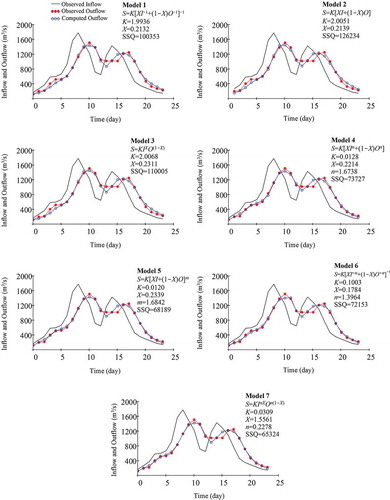
The data for this example are based on Viessman and Lewis (2003). The observed inflow and observed outflow hydrographs, and estimated outflow hydrographs using different models and their corresponding SSQ values, are presented in Table 4 (Δt = 1 d). A comparison of the outflow hydrographs estimated by the proposed models and the observed outflow hydrograph is presented in Fig. 3. The classical linear model 2 and nonlinear model 7 achieve the worst and best SSQ values, respectively, among all applied models. As seen, among the two-parameter models, model 1 (SSQ = 100 353 m⁶/s²) is the most efficient one. The application of the proposed novel model 1 for this example shows that it could improve the fit to observed outflows in comparison to the classical linear Muskingum model 2 (20.5% reduction in SSQ). Among the three-parameter models, the model 7 (SSQ = 65 324 m⁶/s²) is the most efficient. The application of model 7 shows that it could improve the fit to observed outflows in comparison to the popular model proposed by Gill (4.2% reduction in SSQ).

Table 4. Observed hydrographs and estimated outflow hydrographs using different Muskingum models for example 3 (multiple-peak inflow and outflow hydrographs)

Time (d)	Inflow (m^3/s)	Observed outflow (m^3/s)	Model 1	Model 2	Model 3	Model 4	Model 5	Model 6	Model 7
				Computed outflow (m^3/s)
0	166.2	118.4	118.4	118.4	118.4	118.4	118.4	118.4	118.4
1	263.6	197.4	152.5	146.6	149.2	199.2	199.3	180.1	189.8
2	365.3	214.1	213.6	207.5	209.8	279.3	279.6	256.9	268.9
3	580.5	402.1	309.0	294.4	300.6	383.9	385.3	366.3	375.3
4	594.7	518.2	424.4	429.4	425.2	507.1	505.7	475.8	492.2
5	662.6	523.9	506.7	511.0	507.7	565.7	565.0	545.5	556.3
6	920.3	603.1	607.5	597.4	600.3	638.7	640.7	643.0	640.1
7	1568.8	829.7	834.9	787.5	808.9	774.4	796.5	864.9	828.2
8	1775.5	1124.2	1169.2	1166.3	1162.1	1111.8	1109.5	1155.8	1125.4
9	1489.5	1379.0	1405.8	1434.9	1422.8	1384.5	1371.0	1355.6	1362.0
10	1223.3	1509.3*	1434.3	1444.7	1446.0	1429.7	1427.0	1400.2	1420.1
11	713.6	1379.0	1383.9	1310.5	1351.6	1343.2	1367.3	1406.1	1392.7
12	645.6	1050.6	1015.6	1026.5	1025.4	1090.8	1095.3	1052.3	1082.2
13	1166.7	1013.7	864.9	878.9	864.1	914.9	903.8	894.8	891.2
14	1427.2	1013.7	1028.4	1029.4	1023.1	1020.1	1015.8	1036.0	1018.9
15	1282.8	1013.7	1191.1	1207.4	1199.5	1191.3	1184.5	1173.8	1177.7
16	1098.7	1209.1	1224.6	1231.8	1232.1	1228.5	1227.9	1209.2	1222.6
17	764.6	1248.8*	1174.4	1149.4	1167.8	1167.6	1180.0	1178.1	1187.3
18	458.7	1002.4	1018.3	950.7	983.6	972.9	991.1	1045.2	1014.4
19	351.1	713.6	715.2	713.6	717.3	714.1	714.4	708.6	713.8
20	288.8	464.4	517.8	539.9	530.5	502.1	492.8	487.0	490.0
21	228.8	325.6	399.9	418.5	409.3	351.5	343.6	357.5	348.8
22	170.2	265.6	315.2	326.1	320.0	245.0	241.0	265.3	250.5
23	143.0	222.6	238.1	251.3	244.1	180.1	179.6	194.2	183.2
SSQ =			100 353	126 234	110 005	73 727	68 189	72 153	65 324

*Maximum outflows are shown in bold.

Figure 3. Observed and estimated hydrographs for example 3 (double-peak hydrograph) along with estimated optimal parameters for different Muskingum models using the SSQ index (the sum of the squared deviations between observed and computed outflows) as an objective function

For models 1, 2 and 3, the storage parameter K has dimension [T] and may have a value close to the travel time of flood peaks. It is interesting that in all examples these three models yield approximately the same results for K. For the first example, according to observed hydrographs the travel time is 30 h, which is close to the estimated values of K in models 1, 2 and 3. Similarly, for the third example, according to the observed hydrographs the travel time of the first peak is 2 d, which is close to the estimated values of K in models 1, 2 and 3. For the second example, the estimated values of K in models 1, 2 and 3 are about 1.5 times the observed travel time, which is 18 h.

6.4 River Wye outflow hydrograph prediction considering lateral inflow effects

Data for the River Wye (December 1960) are used in this practical example. The computed volume ratio is r = 1.202, thus the lateral inflow may be important in the flood routing procedure. The observed inflow and observed outflow hydrographs, and predicted outflow hydrographs considering lateral flow and using different models are presented in Table 5 (Δt = 6 h). A comparison of the outflow hydrographs predicted by the proposed models and the observed outflow hydrograph is also presented in Fig. 4. The classical linear model 2 and nonlinear model 6 achieve the worst and best SSQ values, respectively, among all applied models. Model 1 (SSQ = 68293 m⁶/s²) is the most efficient two-parameter model. The novel model 1 improves the fit to the observed outflows in comparison to the classical linear Muskingum model 2 (63% reduction in SSQ). Among the three-parameter models considered, model 6 (SSQ = 18363 m⁶/s²) is the most efficient. Model 6 improves the fit to the observed outflows in comparison to the proposed popular model 5 (77.3% reduction in SSQ).

Table 5. Observed hydrographs and estimated outflow hydrographs using different Muskingum models for example 2 by incorporating the lateral inflow r = 1.202 (Non-smooth Single-peak inflow and outflow hydrographs)

Time (h)	Inflow (m^3/s)	Observed Outflow (m^3/s)	Model 1	Model 2	Model 3	Model 4	Model 5	Model 6	Model 7
			Computed Outflow (m^3/s)
0	154	102	102	102	102	102.0	102	102.0	102
6	150	140	114.9	120.3	118.0	148.8	146.0	124.1	141.8
12	219	169	117.0	120.7	115.7	174.2	165.1	139.5	157.1
18	182	190	143.4	158.5	151.1	204.7	203.0	168.2	197.7
24	182	209	153.8	168.5	161.7	199.6	197.3	175.4	193.5
30	192	218	159.7	174.2	166.8	199.5	195.7	179.2	191.4
36	165	210	177.6	187.0	184.8	198.2	198.5	190.5	198.1
42	150	194	182.6	186.2	186.9	182.0	182.3	186.3	182.7
48	128	172	188.5	182.2	187.5	162.3	163.2	180.1	164.8
54	168	149	154.0	162.9	156.4	158.3	153.0	153.4	148.2
60	260	136	146.3	153.1	143.1	190.0	177.9	162.9	168.9
66	471	228	167.2	155.2	152.8	235.4	216.0	206.5	209.3
72	717	303	225.7	215.1	208.2	300.4	277.3	280.7	273.5
78	1092	366	320.1	312.1	297.8	302.4	314.4	377.7	335.4
84	1145	456	452.8	545.5	466.4	545.4	474.5	482.8	446.1
90	600	615	672.4	822.4	773.5	806.3	780.2	612.7	706.3
96	365	830	902.1	807.2	869.4	791.8	827.4	847.6	856.4
102	277	969*	841.8	702.3	768.3	720.6	765.8	944.1	831.5
108	227	665	665.4	594.6	635.2	634.9	672.5	725.7	723.9
114	187	519	532.4	500.8	523.0	542.8	567.4	535.1	587.7
120	161	444	414.8	419.3	423.8	447.2	454.0	378.9	434.8
126	143	321	329.3	351.8	344.8	353.1	343.1	281.6	302.8
132	126	208	275.7	297.9	287.7	266.0	246.9	224.1	211.9
138	115	176	229.4	253.2	240.4	193.0	175.3	180.3	156.7
144	102	148	201.5	218.1	207.5	143.2	134.4	153.1	127.8
150	93	125	174.2	188.5	178.6	115.5	112.3	129.7	109.6
156	88	114	149.8	163.9	154.1	102.3	100.9	112.1	99.1
162	82	106	134.3	145.0	136.9	93.6	92.7	101.2	91.3
168	76	97	122.3	129.6	123.4	86.2	85.5	92.4	84.4
174	73	89	109.7	116.2	110.7	82.1	81.8	84.5	80.4
180	70	81	100.6	105.8	101.2	78.5	78.7	79.2	77.0
186	67	76	93.6	97.4	93.7	75.3	76.2	75.1	74.1
192	63	71	88.6	90.7	88.1	71.3	74.0	71.5	70.8
198	59	66	83.9	84.6	83.0	68.5	78.7	67.4	69.7
SSQ =			68 293	184 467	120 910	122 705	80 946	18 363	43 085

*Maximum outflows are shown in bold.

Figure 4. Observed and estimated hydrographs for example 2 considering inflow effects (non-smooth single-peak hydrograph) along with estimated optimal parameters for different Muskingum models using the SSQ index (the sum of the squared deviations between observed and computed outflows) as an objective function

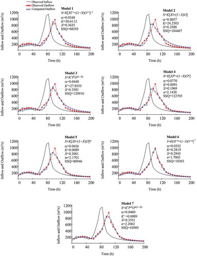
By incorporating the lateral flow (α = 0.0348), the novel model 1 improves the fit to the observed outflows in comparison to the case without lateral flow (α = 0; 4.8% reduction in SSQ). Similarly, by incorporating the lateral flow (α = 0.0352), the novel model 6 improves the fit to the observed outflows in comparison to the case without lateral flow (α = 0; 16.8% reduction in SSQ).

6.5 River Wye outflow hydrograph prediction from January 1969 data

Data for the River Wye (January 1969) are reported by O’Donnell (1985) and used in this practical example. The peak outflow discharge for this flood is 323 m³/s, which occurs at t = 60 h. The computed volume ratio for this flood is r = 0.994, thus the lateral flow has no effect on the flood routing procedure. This issue shows that the river reach condition changed after 10 years (from December 1960 to January 1969), and thus the optimal model parameters of the River Wye data for December 1960 cannot be used to accurately predict the outflow hydrograph for the current flood (January 1969). According to example 2, model 6 is more efficient than the others for this river. Recalibrating model 6 using the River Wye data (January 1969) yields K = 0.0915, X = 0.4600 and n = 1.8224 (SSQ = 6164 m⁶/s²). According to the outflow hydrograph computed by model 6 (using K = 0.0915, X = 0.4600 and n = 1.8224), the peak outflow discharge is 322.7 m³/s, which occurs at t = 60 h. As noted, both peak time and peak outflow discharge were correctly predicted.

7 Conclusions

This study proposes a general form for the storage function in the Muskingum model, showing a good application of mathematics to hydrologic engineering. Based on this research, the following comments are offered.

1. The proposed model is based on the assumption that the relationship of the storage is a weighted power mean between the storage volumes due to the inflow and outflow rather than the weighted arithmetic mean, which is traditionally assumed. This approach presents an improvement over other existing representations of channel storage based on the weighted arithmetic mean.

2. The proposed model combines all existing dimensionally homogeneous forms of the storage equation in a unified form, and all existing forms of the Muskingum model are special cases of the proposed general model.

3. The general mathematically based form of Equation (10)(10) $S=[X(S_{in}{)}^p+\left(1-X\right)(S_{out}{)}^p{]}^{\frac{1}{p}}$(10) makes possible the derivation of some new, original and efficient nonlinear storage equations. This model can be expressed in two general forms as K[XIⁿ + (1 − X)Oⁿ]^m and KI^nXO^n(1−X), the parameters of which can be set to produce different desired models with fewer parameters. These two general forms provide the user with flexibility in evaluating all models easily and can be simply implemented using Microsoft Excel spreadsheets (used in this study) or any programming software that employs optimization algorithms. The Excel Solver tool uses a powerful search process called the generalized reduced gradient (GRG), which is not a local search technique. It provides global optimal solutions easily and within a short time. The failure of the calibration process should be prevented by the penalty function approach. The proposed general model reduces to two novel harmonic storage models (K[XI⁻¹ + (1 − X)O⁻¹]⁻¹ and K[XI⁻ⁿ + (1 − X)O⁻ⁿ]⁻¹), and two novel geometric storage models (KI^XO^(1−X) and KI^nXO^n(1−X)), which have not been reported before (n > 0). The proposed Muskingum models can also take lateral flow into consideration.

4. It is important to asses all the possible forms to get a global view of the abilities of this kind of model. By considering new storage equations, it is possible to select the most efficient equation for a given natural river. It should be noted that a storage equation with fewer model parameters should be selected, as far as possible without losing accuracy in the outflow prediction.

5. The SSQ index is used as an objective function for optimal parameter estimation and as a model performance evaluation criterion. Different numerical solution methods can be used to solve the governing equations. In this study the proposed Muskingum models are solved using the fourth-order Runge-Kutta method as an accurate numerical solution method.

6. The SSQ reduction of the new proposed models varies with the type of observed hydrographs. For the three practical examples considered in this study, the maximum reductions in SSQ for the new two-parameter models in comparison to the classical linear Muskingum model are 84.2% (example 1), 63.4% (example 2) and 20.5% (example 3). The maximum reductions in SSQ for the new three-parameter models in comparison to Gill’s popular model are 36.4% (example 1), 76.1% (example 2) and 4.2% (example 3). The results showed that the new proposed storage models significantly improve the Muskingum model performance in comparison to the traditional storage models.

7. In different storage models, it is assumed that the overall flood-attenuating characteristics of a given river reach remain constant and independent of the flooding event. As a result, flood-attenuating characteristics determined for a specified flood event using a set of observed inflow–outflow hydrographs (captured by the model parameters) can be used for routing any future outflow hydrographs for the river reach under study (if river condition and geometry remain unchanged). According to this assumption, the average hydraulic behaviour of a given river reach will be captured by the model parameters, and every river reach will have its own model parameters according to a historic set of observed inflow–outflow hydrographs and used storage model. Since every given river reach has its own model parameters, it is not possible to suggest any criterion for the selection of a storage equation for flood routing of a given river reach.

Disclosure statement

No potential conflict of interest was reported by the author.

Appendix.

Analytical derivation of S when p tending to 0 (Equation (13))

Since functions e^x and ln(x) are the inverse of each other and both are continuous (e^ln(x) = x), Equation (13)(13) $S=\underset{p\to 0^{+}}{lim}\left\{K{[X{I}^{np}+\left(1-X\right)O^{np}]}^{\frac{1}{p}}\right\}=K{I}^{nX}{O}^{n\left(1-X\right)}$(13) can thus be written as:

$\begin{array}{rl}& S=\underset{p\to 0^{+}}{lim}\left\{K{[X{I}^{np}+(1-X)O^{mp}]}^{\frac{1}{p}}\right\}\\ & =e^{ln\left(\underset{p\to 0^{+}}{lim}\left\{K{[X{I}^{np}+(1-X)O^{mp}]}^{\frac{1}{p}}\right\}\right)}\\ & =e^{\underset{p\to 0^{+}}{lim}ln\left\{K{[X{I}^{np}+(1-X)O^{mp}]}^{\frac{1}{p}}\right\}}\\ & =e^{lnK}{e}^{\underset{p\to 0^{+}}{lim}ln\left\{{[X{I}^{np}+(1-X)O^{mp}]}^{\frac{1}{p}}\right\}}\\ & =K{e}^{\underset{p\to 0^{+}}{lim}\frac{ln[X{I}^{np}+(1-X)O^{mp}]}{p}}\end{array}$

Since the limit is of the form 0/0, L’Hopital’s rule can be used as the following:

$\begin{array}{rl}& S=K{e}^{\underset{p\to 0^{+}}{lim}\frac{\frac{X{I}^{np}ln(I^n)+(1-X)O^{mp}ln(O^n)}{X{I}^{np}+(1-X)O^{mp}}}{1}}\\ & =K{e}^{\frac{Xln(I^n)+(1-X)ln(O^n)}{X+(1-X)}}\\ & =K{e}^{[ln(I^{nX})+ln(O^{n(1-X)})]}\\ & =K{e}^{[ln(I^{nX}{O}^{n(1-X)})]}\\ & =K{I}^{nX}{O}^{n(1-X)}\end{array}$

References

- Akan, A.O., 2006. Open channel hydraulics. Oxford, UK: Butterworth-Heinemann.
- Akbari, G.H. and Barati, R., 2012. Comprehensive analysis of flooding in unmanaged catchments. Proceedings of the ICE-Water Management, 165 (4), 229–238. doi:https://doi.org/10.1680/wama.10.00036
- Akbari, R., Hessami-Kermani, M.R., and Shojaee, S., 2020. Flood routing: improving outflow using a new non-linear Muskingum model with four variable parameters coupled with PSO-GA algorithm. Water Resources Management, 34 (10), 3291–3316. doi:https://doi.org/10.1007/s11269-020-02613-5
- Ayvaz, M.T. and Gurarslan, G., 2017. A new partitioning approach for nonlinear Muskingum flood routing models with lateral flow contribution. Journal of Hydrology, 553, 142–159. doi:https://doi.org/10.1016/j.jhydrol.2017.07.050
- Barat, R., Akbari, G.H., and Rahimi, S., 2013. Flood routing of an unmanaged River Basin using Muskingum-Cunge model; field application and numerical experiments. Caspian Journal of Applied Sciences Research, 2 (6), 8–20.
- Barati, R., 2013. Application of excel solver for parameter estimation of the nonlinear Muskingum models. KSCE Journal of Civil Engineering, 17 (5), 1139–1148. doi:https://doi.org/10.1007/s12205-013-0037-2
- Barati, R., Rahimi, S., and Akbari, G.H., 2012. Analysis of dynamic wave model for flood routing in natural rivers. Water Science and Engineering, 5 (3), 243–258.
- Barati, R., et al., 2014. Discussion: new and improved four-parameter non-linear Muskingum model. Proceedings of the ICE-Water Management, 167 (10), 612–615.
- Bazargan, J. and Norouzi, H., 2018. Investigation the effect of using variable values for the parameters of the linear Muskingum method using the Particle Swarm Algorithm (PSO). Water Resources Management, 32 (14), 4763–4777. doi:https://doi.org/10.1007/s11269-018-2082-6
- Beven, K.J., 2011. Rainfall-runoff modelling: the primer. Oxford, UK: John Wiley & Sons.
- Bozorg-Haddad, O., et al., 2019. Generalized storage equations for flood routing with nonlinear Muskingum models. Water Resources Management, 33 (8), 2677–2691. doi:https://doi.org/10.1007/s11269-019-02247-2
- Chow, V.T., 1959. Open channel hydraulics. New York, NY: McGraw-Hill.
- Chu, H.J. and Chang, L.C., 2009. Applying particle swarm optimization to parameter estimation of the nonlinear Muskingum model. Journal of Hydrologic Engineering, 14 (9), 1024–1027. doi:https://doi.org/10.1061/(ASCE)HE.1943-5584.0000070
- Easa, S.M., 2013. Improved nonlinear Muskingum model with variable exponent parameter. Journal of Hydrologic Engineering, 18 (12), 1790–1794. doi:https://doi.org/10.1061/(ASCE)HE.1943-5584.0000702
- Easa, S.M., 2014a. Closure to “improved nonlinear Muskingum model with variable exponent parameter” by Said M. Easa. Journal of Hydrologic Engineering, 19 (10), 07014008. doi:https://doi.org/10.1061/(ASCE)HE.1943-5584.0001041
- Easa, S.M., 2014b. New and improved four-parameter nonlinear Muskingum model. Proceedings of the ICE–Water Management, 167 (5), 288–298.
- Easa, S.M., 2015a. Versatile Muskingum flood model with four variable parameters. Proceedings of the ICE-Water Management, 168 (3), 139–148. doi:https://doi.org/10.1680/wama.14.00034
- Easa, S.M., 2015b. Evaluation of nonlinear Muskingum model with continuous and discontinuous exponent parameters. KSCE Journal of Civil Engineering, 19 (7), 2281–2290. doi:https://doi.org/10.1007/s12205-015-0154-1
- Gavilan, G. and Houck, M.H., 1985. Optimal Muskingum river routing. In: Specialty Conference: Computer applications in water resources. Buffalo, NY: ASCE, 1294–1302.
- Geem, Z.W., 2006. Parameter estimation for the nonlinear Muskingum model using the BFGS technique. Journal of Hydrologic Engineering, 474–478. doi:https://doi.org/10.1061/(ASCE)0733-9437(2006)132:5(474)
- Geem, Z.W., 2011. Parameter estimation of the nonlinear Muskingum model using parameter-setting-free harmony search. Journal of Hydrologic Engineering, 16 (8), 684–688. doi:https://doi.org/10.1061/(ASCE)HE.1943-5584.0000352
- Gill, M.A., 1978. Flood routing by the Muskingum method. Journal of Hydrology, 36 (3–4), 353–363. doi:https://doi.org/10.1016/0022-1694(78)90153-1
- Karahan, H., 2014. Discussion of “improved nonlinear Muskingum model with variable exponent parameter” by Said M Easa. Journal of Hydrologic Engineering, 14, 1–9. doi:https://doi.org/10.1061/(ASCE)HE.1943-5584.0000702
- Karahan, H., Gurarslan, G., and Geem, Z.W., 2013. Parameter estimation of the nonlinear Muskingum flood-routing model using a hybrid harmony search algorithm. Journal of Hydrologic Engineering, 18 (3), 352–360. doi:https://doi.org/10.1061/(ASCE)HE.1943-5584.0000608
- Karahan, H., Gurarslan, G., and Geem, Z.W., 2015. A new nonlinear Muskingum flood routing model incorporating lateral flow. Engineering Optimization, 47 (6), 737–749. doi:https://doi.org/10.1080/0305215X.2014.918115
- Kim, J.H., Geem, Z.W., and Kim, E.S., 2001. Parameter estimation of the nonlinear muskingum model using harmony search. Journal of the American Water Resources Association, 37 (5), 1131–1138. doi:https://doi.org/10.1111/j.1752-1688.2001.tb03627.x
- Luo, J. and Xie, J., 2010. Parameter estimation for nonlinear Muskingum model based on immune clonal selection algorithm. Journal of Hydrologic Engineering, 15 (10), 844–851. doi:https://doi.org/10.1061/(ASCE)HE.1943-5584.0000244
- McCarthy, G.T., 1938. The unit hydrograph and flood routing. In: Proceeding of the Conference of North Atlantic Division, U.S. Army Corps of Engineers. Washington, DC.
- Mohan, S., 1997. Parameter estimation of nonlinear Muskingum models using genetic algorithm. Journal of Hydraulic Engineering, 123 (2), 137–142. doi:https://doi.org/10.1061/(ASCE)0733-9429(1997)123:2(137)
- NERC (Natural Environment Research Council), 1975. Flood studies report, Vol. III. Wallingford, UK: Institute of Hydrology.
- Niazkar, M. and Afzali, S.H., 2017. New nonlinear variable-parameter Muskingum models. KSCE Journal of Civil Engineering, 21 (7), 2958–2967. doi:https://doi.org/10.1007/s12205-017-0652-4
- O’Donnell, T., 1985. A direct three-parameter Muskingum procedure incorporating lateral inflow. Hydrological Sciences Journal, 30 (4), 479–496. doi:https://doi.org/10.1080/02626668509491013
- Qi, F., et al., 2000. New proofs of weighted power mean inequalities and monotonicity for generalized weighted mean values. Mathematical Inequalities & Applications, 3 (3), 377–383.
- Vatankhah, A.R., 2010. Discussion of ‘applying particle swarm optimization to parameter estimation of the nonlinear Muskingum model’ by H.-J. Chu and L.-C. Chang. Journal of Hydrologic Engineering, 15 (11), 949–952. doi:https://doi.org/10.1061/(ASCE)HE.1943-5584.0000211
- Vatankhah, A.R., 2014a. Evaluation of explicit numerical solution methods of the Muskingum model. Journal of Hydrologic Engineering, 19 (8), 06014001. doi:https://doi.org/10.1061/(ASCE)HE.1943-5584.0000978
- Vatankhah, A.R., 2014b. Discussion of “improved nonlinear Muskingum model with variable exponent parameter” by Said M. Easa. Journal of Hydrologic Engineering, 19 (10), 07014004. doi:https://doi.org/10.1061/(ASCE)HE.1943-5584.0001044
- Vatankhah, A.R., 2014c. Discussion of ‘parameter estimation of the nonlinear Muskingum flood-routing model using a hybrid harmony search algorithm’ by Halil Karahan, Gurhan Gurarslan, and ZongWoo Geem. Journal of Hydrologic Engineering, 19 (4), 839–842. doi:https://doi.org/10.1061/(ASCE)HE.1943-5584.0000845
- Vatankhah, A.R., 2015a. Discussion of “application of excel solver for parameter estimation of the nonlinear Muskingum models” by Reza Barati. KSCE Journal of Civil Engineering, 19 (1), 332–336. doi:https://doi.org/10.1007/s12205-014-1422-1
- Vatankhah, A.R., 2015b. Discussion of “parameter estimation for the nonlinear forms of the Muskingum model” by Piyusha Hirpurkar and Aniruddha D. Ghare. Journal of Hydrologic Engineering, 20 (11), 07015018. doi:https://doi.org/10.1061/(ASCE)HE.1943-5584.0001187
- Vatankhah, A.R., 2017. Non-linear Muskingum model with inflow-based exponent. Proceedings of the ICE-Water Management, 170 (2), 66–80. Thomas Telford Ltd.
- Vatankhah, A.R., 2018. Discussion of “assessment of modified Honey Bee mating optimization for parameter estimation of nonlinear Muskingum models” by Majid Niazkar and Seied Hosein Afzali. Journal of Hydrologic Engineering, 23 (4), 07018002. doi:https://doi.org/10.1061/(ASCE)HE.1943-5584.0001603
- Viessman, W. and Lewis, G.L., 2003. Introduction to hydrology. NJ, USA: Pearson.
- Wilson, E.M., 1974. Engineering hydrology. Hampshire, UK: MacMillan Education.
- Xu, D.M., Qiu, L., and Chen, S.Y., 2012. Estimation of nonlinear Muskingum model parameter using differential evolution. Journal of Hydrologic Engineering, 17 (2), 348–353. doi:https://doi.org/10.1061/(ASCE)HE.1943-5584.0000432
- Yoon, J.W. and Padmanabhan, G., 1993. Parameter-estimation of linear and nonlinear Muskingum models. Journal of Water Resources Planning and Management, 119 (5), 600–610. doi:https://doi.org/10.1061/(ASCE)0733-9496(1993)119:5(600)