On the role of floodplain storage and hydrodynamic interactions in flood risk estimation

ABSTRACT

Hydrodynamic interactions, i.e. the floodplain storage effects caused by inundations upstream on flood wave propagation, inundation areas, and flood damage downstream, are important but often ignored in large-scale flood risk assessments. Although new methods considering these effects sometimes emerge, they are often limited to a small or meso scale. In this study, we investigate the role of hydrodynamic interactions and floodplain storage on flood hazard and risk in the German part of the Rhine basin. To do so, we compare a new continuous 1D routing scheme within a flood risk model chain to the piece-wise routing scheme, which largely neglects floodplain storage. The results show that floodplain storage is significant, lowers water levels and discharges, and reduces risks by over 50%. Therefore, for accurate risk assessments, a system approach must be adopted, and floodplain storage and hydrodynamic interactions must carefully be considered.

KEYWORDS:

• hydrodynamic interactions
• derived flood risk analysis
• flood modelling
• Rhine basin

Editor A. Castellarin Associate Editor A. Domeneghetti

1 Introduction

Large-scale flood risk assessments are needed for national policy developments, disaster management planning, and the insurance industry (de Moel et al. 2015). However, studies presenting large-scale flood risk assessments are still rare and suffer from data and methodological limitations regarding the realistic representation of hydrodynamic interactions (Vorogushyn et al. 2018).

With hydrodynamic interactions, we understand changes in discharge, water levels, and, consequently, hazard and risk downstream of the river network due to inundation and water storage in the upstream reaches. Hence, the term includes lateral interactions between the river channel and the floodplains and longitudinal interactions between upstream and downstream locations. Concrete examples are the discharge-reducing effects of flooding due to the overflow of embankments or breaches and detention areas. Such interactions are complex and depend on several factors, including floodplain topography, the presence of dikes, and their failures. Floodplain topography determines the amount of stored water and thus flood wave attenuation. Dike failures result in flooding of protected floodplains which, in turn, affects flood hazards of areas downstream.

A common approach for large-scale flood mapping and risk assessment is based on the estimation of peak discharge values associated with certain return periods at gauge locations, which are subsequently used as boundary conditions for hydrodynamic simulations. The results of these local simulations are mosaicked into a large-scale picture (“mosaic approach”). Some approaches use uniform return periods to estimate peak flows for entire countries (Bradbrook et al. 2005, Merz et al. 2008) or even continents (Alfieri et al. 2014). The assumption of a uniform return period, if used for risk assessments of larger areas, contravenes the basic spatial dependence structure of floods and leads to an overestimation of flood damage for high return periods (Vorogushyn et al. 2018, Metin et al. 2020, Nguyen et al. 2020). The expected annual damage is, however, not necessarily affected by the homogeneous return period assumption (Metin et al. 2020). Recently, several studies used multivariate extreme value models for estimating peak discharges (Keef et al. 2009, Lamb et al. 2010, Ward et al. 2013, Jongman et al. 2014, Wyncoll and Gouldby 2015, Quinn et al. 2019, Winter et al. 2019). These approaches generate patterns of spatially dependent peak flows at multiple gauges with heterogeneous return periods.

To use peak flows (with homogeneous or heterogeneous return periods) for unsteady hydrodynamic simulations, assumptions about the flow hydrographs are needed, e.g. typical hydrograph shapes scaled to the predefined peak magnitude. Hydrodynamic simulations are then carried out for individual reaches, i.e. piece-wise, whereas a new boundary condition is assigned at the next downstream gauge (e.g. Alfieri et al. 2016, Falter et al. 2016, Quinn et al. 2019). This approach is valid only for a single river reach. In a larger river network, it results in inconsistent, non-mass conservative sets of flood hydrographs, inundation areas, and risk estimates (Curran et al. 2020). Reach-wise or piece-wise routing is still common for many large-scale risk assessment studies (Alfieri et al. 2016, Quinn et al. 2019).

Flood hazard and risk assessment approaches considering hydrodynamic interactions have emerged in recent years and deploy continuous hydrodynamic simulations along a single river reach or in a larger river network. These approaches account for floodplain storage effects caused by inundation considering or disregarding dike failures. Apel et al. (2004) and Vorogushyn et al. (2010, 2012) indicated the effect of hydrodynamic interactions on flood hazard and risk at the Lower Rhine and a small reach of the Elbe River, respectively, due to dike failures. Apel et al. (2009), for instance, showed that the design flood at the German–Dutch border is significantly reduced when dike breaches are stochastically considered, compared to the gauge-based extreme value statistics, which does not fully account for hydrodynamic interactions. Van Mierlo et al. (2007) indicated the effect of hydrodynamic interactions for a dike ring in the Rhine-Meuse delta. de Bruijn et al. (2014) compared scenarios with and without hydrodynamic interactions for the entire Rhine-Meuse delta in terms of the number of simulated dike breaches and resulting estimates of flood fatalities. They showed that the estimated annual probability of life loss is more than doubled in the scenario without considering dike failures. Curran et al. (2019) continued their work and improved the method by better representing floodplain flows. Recently, Ciullo et al. (2019) demonstrated how hydrodynamic interactions resulting from dike breaches in the IJssel River in the Netherlands affect the optimal dike height in a cost–benefit framework. They concluded that disregarding the dike failures’ mutual dependence results in sub-optimal design height and increased overall costs. Dupuits et al. (2019) came to the same conclusion using a similar setting applied for a case study in a small region in the Netherlands. These approaches, however, have used one or very few locations to define the boundary conditions for hydrodynamic models, and do not consider the upstream part of the catchment with several tributaries and rainfall distribution issues. Hydrodynamic interactions are expected to gain importance with increasing spatial scale and numbers of tributaries and in lowland rivers with large floodplain storage capacities (Vorogushyn et al. 2018). Hence, there is a need to consider hydrodynamic interactions for large-scale risk assessments.

Although the role of the floodplain in attenuating floods in large-scale basins is generally understood (Yamazaki et al. 2011, 2012, De Paiva et al. 2013) the implications for flood risk are not well investigated. Fleischmann et al. (2019) have investigated the role of the floodplains in large-scale catchments using the MGB inline coupled hydrological–hydrodynamic model. They concluded that the absence of right floodplain representation in the model would lead to an expressive discharge overestimation with higher peaks and faster recession limbs. A continuous simulation approach represents an alternative way to estimate flood hazard and risk for large-scale basins compared to the mosaic approach. It is based on a model chain covering the whole flood hazard/risk process cascade from heterogeneous patterns of precipitations to runoff generation in the catchments and river discharge down to inundation and damage. This approach, termed “Derived Flood Risk Analysis” (Falter et al. 2015), extends the “Derived Flood Frequency Approach based on continuous simulation” (e.g. Blazkova and Beven 2004) often used for flood design estimation. Hence, depending on the goal, the model chain can be truncated and can focus on discharge or flood frequency estimation (Haberlandt and Radtke 2014, Hegnauer et al. 2014), inundation area estimation (Grimaldi et al. 2013) or flood damage and risk assessment (Falter et al. 2015, 2016). The model chain is driven with observed or synthetic climate data, e.g. provided by a stochastic weather generator. The rainfall-runoff modelling provides flow hydrographs at specific locations, which are used as boundary conditions for hydrodynamic flood simulations. Contrary to the gauge-based multisite models, this approach delivers spatially consistent, mass-conservative, and time-continuous flow hydrographs at multiple locations (depending on the structure and resolution of the hydrological models). These continuous flow hydrographs are used as upstream and lateral boundary conditions for continuous hydrodynamic simulations considering hydrodynamic interactions.

Continuously coupled rainfall-runoff and hydrodynamic simulations are state-of-the-art (e.g. Biancamaria et al. 2009, De Paiva et al. 2013, Hegnauer et al. 2014), but they are so far rarely deployed for large-scale flood risk assessments due to their complexity and computational constraints. Winsemius et al. (2013) used a global hydrological model coupled to a kinematic wave-routing scheme with simplified inundation approximation for past damage reanalysis. Two-dimensional (2D) hydrodynamic models are particularly computationally demanding when it comes to the long-term simulation of multiple scenarios needed for risk assessments. To our knowledge, there exists no large-scale risk analysis based on a continuous hydrological–hydrodynamic simulation driven by a long-term weather generator.

In the present study, we analyse the effect of hydrodynamic interactions on flood hazard and risk assessment for the Rhine basin (185 260 km²). In particular, we focus on the importance of these interactions with increasing basin scale by comparing (1) flood flows, (2) overtopping volumes, (3) inundation patterns, and (4) damage to residential, commercial, and agricultural sectors. The comparison is made between assessments with and without consideration of floodplain storage and interactions at different locations upstream and downstream of the basin by comparing two model chains: one based on a sub-basin-wise river routing and a fully continuous hydrodynamic approach. Indeed, there are several studies focussing on modelling floodplain flow, but they do not quantify the effect on flood risk. The contribution of our study is to address how this interaction results in redistribution not only of the hazard part (similar to previous studies) but also the estimated damage and risk.

The paper is organized as follows. Section 2 provides a detailed description of the RFM model chain using a piece-wise routing and a newly implemented continuous routing. The model set-up for the Rhine case study, input data for each component of the RFM model chain, and the design of the computational experiments are detailed in Section 3, followed by a discussion of the results and conclusions in sections 4 and 5, respectively. The cross-section data derivation and extensive model validation, including a comparison of simulated maximum annual discharge/water levels against observations, are presented in detail in the Appendix.

2 Methods

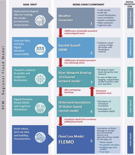
For the analysis of hydrodynamic interactions, we use the Regional Flood Model (RFM; Falter et al. 2015, 2016), representing a model chain for time-continuous, spatially consistent simulation of flood processes from atmospheric input to flood damage and risk. It consists of several components, including the multisite, multivariate regional weather generator (RWG; Hundecha et al. 2009, Nguyen et al. 2021), the SWIM rainfall-runoff model (Krysanova et al. 1998), a one-dimensional (1D) river routing model based on diffusive wave approximation coupled to a 2D raster-based hinterland inundation model (Falter et al. 2015, 2016), and the FLEMO flood loss estimation model (Thieken et al. 2008, Kreibich et al. 2010; Fig. 1).

Figure 1. RFM modelling framework: components, input data requirements, and spatial discretization.

2.1 Regional weather generator

The multisite, multivariate RWG is a stochastic model that generates daily time series of precipitation at multiple locations. Based on the state of the generated precipitation (dry/wet), the RWG then generates non-precipitation variables such as temperature (minimum, average, and maximum), relative humidity, and solar radiation. RWG was introduced by Hundecha et al. (2009) and was recently comprehensively evaluated by Nguyen et al. (2021). RWG assumes that extreme precipitation events have different stochastic behaviour compared to the normal precipitation regime. Hence, it uses a mixed distribution, i.e. a gamma distribution for bulk precipitation and a more heavy-tailed generalized Pareto distribution for extreme precipitation. The spatial and temporal dependence is represented by a first-order multivariate autoregressive model considering the spatial covariance structure.

The distribution of the full range of precipitation (including zero precipitation) is formulated by combining the mixed distribution and the frequency of non-zero precipitation. For relative humidity and the temperature variables, the normal distribution is used. For solar radiation, the square-root transformed data are fitted to the normal distribution due to its relatively strong right skewness. RWG is parameterized on a monthly basis to account for seasonality.

2.2 Rainfall-runoff model (SWIM)

The hydrological model SWIM (Soil and Water Integrated Model; Krysanova et al. 1998) is a conceptual semi-distributed rainfall-runoff model for mesoscale catchments. SWIM computes average daily runoff at sub-basin spatial discretization. Each sub-basin is further sub-divided into hydrological response units or hydrotopes, where soil type, land use, and average water table depth are assumed to be homogeneous. Runoff is calculated for each hydrotope and then aggregated on a sub-basin scale. SWIM is driven by daily precipitation, maximum and minimum air temperature, relative humidity, and solar radiation. SWIM relies on the water balance equation considering snow, precipitation, evapotranspiration, percolation, surface and subsurface runoff, recharge, and capillary rise. The model applies the SCS curve number method for surface runoff volume estimation. For the routing between sub-basins, the Muskingum routing approach is used (Cunge 1969).

2.3 Regional Inundation Model

The Regional Inundation Model (RIM) consists of a 1D hydrodynamic routing model coupled with a 2D hinterland inundation model. The 1D hydrodynamic model solves the diffusive wave approximation of the shallow water equations (SWEs) (Equations 1(1) $\frac{\mathrm{\partial }Q}{\mathrm{\partial }t}+\frac{\mathrm{\partial }}{\mathrm{\partial }x}\left(\frac{Q^2}{A}\right)+gA\frac{\mathrm{\partial }h}{\mathrm{\partial }x}-gA\left(S_o-S_f\right)=0$(1) and 2(2) $\frac{\mathrm{\partial }Q}{\mathrm{\partial }x}+\frac{\mathrm{\partial }A}{\mathrm{\partial }t}=0$(2) ), where the first two terms (local and advective acceleration) are neglected in the momentum equation (Equation 1):

(1) $\frac{\mathrm{\partial }Q}{\mathrm{\partial }t}+\frac{\mathrm{\partial }}{\mathrm{\partial }x}\left(\frac{Q^2}{A}\right)+gA\frac{\mathrm{\partial }h}{\mathrm{\partial }x}-gA\left(S_o-S_f\right)=0$(1)

(2) $\frac{\mathrm{\partial }Q}{\mathrm{\partial }x}+\frac{\mathrm{\partial }A}{\mathrm{\partial }t}=0$(2)

where Q is the discharge (m³ s⁻¹), A is the cross-section area (m²), g is the gravitational acceleration (m s⁻²), $S_o$ is the bed slope (m⁻¹), $S_f$ is the friction slope (m⁻¹), x is the distance (m), and t is the time (s).

An explicit finite difference scheme is used to solve the equations with adaptive time steps following the Courant-Friedrichs-Lewy criterion to secure numerical model stability. However, numerical instabilities may occur due to a sudden increase in the value of the wetted perimeter (P) with a minimal increase in water depth. Such instabilities may happen when the water level exceeds the bankfull area, and overbank flow occurs. Fread (1976) and Smith (1978) solved this problem by dividing the system into two separate conveying systems, i.e. a compound channel. We adopted this solution following Equation (3)(3) $\frac{\mathrm{\partial }{Q}_{bf}}{\mathrm{\partial }x}+\frac{\mathrm{\partial }{A}_{bf}}{\mathrm{\partial }t}+\frac{\mathrm{\partial }{Q}_{Overbank}}{\mathrm{\partial }x}+\frac{\mathrm{\partial }{A}_{Overbank}}{\mathrm{\partial }t}=0$(3) :

(3) $\frac{\mathrm{\partial }{Q}_{bf}}{\mathrm{\partial }x}+\frac{\mathrm{\partial }{A}_{bf}}{\mathrm{\partial }t}+\frac{\mathrm{\partial }{Q}_{Overbank}}{\mathrm{\partial }x}+\frac{\mathrm{\partial }{A}_{Overbank}}{\mathrm{\partial }t}=0$(3)

where $Q_{bf}$ is the discharge conveyed within the channel (m³ s⁻¹), A_bf is the bankfull (m²) area, and $Q_{Overbank}$ is the discharge (m³ s⁻¹) conveyed through A_overbank, the overbank area (m²).

The deployed solution of the SWEs uses water depth as an upstream boundary condition. Therefore, the flow hydrograph resulting from summing up all the upstream flow (lateral and upstream river branch) is converted into the water depth using Manning’s equation for the first cross-section in each sub-basin. To establish a stage–discharge relationship, the bed slope and hence cross-section bankfull depth are calibrated.

The 1D model uses simplified cross-section data that consist of two components: overbank river geometry and bankfull area. The cross-sections represent the river geometry between left and right dike crests or elevated banks. The overbank geometry is represented by the trapezoidal shape described by six points. Model discretization and derivation of cross-sections are detailed in the Appendix.

In this study, we use two implementations of the 1D hydrodynamic model to quantify the effect of hydrodynamic interactions. In the original model version (RIM1.0), a piece-wise routing of overbank flow was implemented (Falter et al. 2015, 2016) (see Appendix, Fig. A2(a)). The bankfull depth is not explicitly represented in the cross-sections (see Appendix, Fig. A3). Discharge corresponding to the bankfull depth is subtracted at the upstream node of each sub-basin, where runoff from the SWIM model is assigned as a boundary condition. Hence, floodplain storage effects due to dike overtopping and inundation, i.e. hydrodynamic interactions, are considered only within single sub-basins and are not propagated across the sub-basin boundaries.

Further, a continuous routing approach (RIM2.0) is implemented (see Appendix, Fig. A2(b)), which is based on the full cross-section geometry, i.e. rectangular bankfull area and trapezoidal overbank geometry (see Appendix, Fig. A3). The flow is continuously routed through the entire river network. In this way, storage effects due to dike overtopping and floodplain inundation on downstream flow hydrographs can be explicitly accounted for. RIM2.0 uses the same computational engine as RIM1.0 based on the explicit solution of the diffusive wave equation. The derivation of cross-sections for both RIM1.0 and RIM2.0 models is detailed in the Appendix.

The 2D hinterland inundation model is deployed when water levels in the river channel overtop dike crests. The outflow into the hinterland is calculated with the broad crested weir equation and provided as a boundary condition for the inundation model. The connection between 1D and 2D models is one-way, where no return flow from the 2D model to the 1D channel is currently accounted for. As soon as the water level in the river channel drops below the crest level, no further overtopping flow is simulated. The 2D hinterland inundation model solves Equations (1)(1) $\frac{\mathrm{\partial }Q}{\mathrm{\partial }t}+\frac{\mathrm{\partial }}{\mathrm{\partial }x}\left(\frac{Q^2}{A}\right)+gA\frac{\mathrm{\partial }h}{\mathrm{\partial }x}-gA\left(S_o-S_f\right)=0$(1) and (2(2) $\frac{\mathrm{\partial }Q}{\mathrm{\partial }x}+\frac{\mathrm{\partial }A}{\mathrm{\partial }t}=0$(2) ) in two dimensions with a neglected advection acceleration term. The 2D model domain is discretized into a regular grid to compute fluxes q per unit width in both directions, x and y and update water depths h in each raster cell (i, j). The explicit solution for q proposed by Bates et al. (2010) reads:

(4) $q_{t+\mathrm{\Delta }t}=\frac{q_t-g{h}_{flow}\mathrm{\Delta }t{S}_f}{\left(1+g{h}_{flow}\mathrm{\Delta }t{n^2}_{\left|q_t\right|}{/}_{h_{flow}}\frac{10}{3}\right)}$(4)

(5) $\frac{\mathrm{\Delta }{h}^{i,j}}{\mathrm{\Delta }t}=\frac{q_x^{i-1,j}-q_x^{i,j}+q_y^{i-1,j}-q_y^{i,j}}{\mathrm{\Delta }x}$(5)

(6) $\mathrm{\Delta }{t}_{max}=\alpha \frac{\mathrm{\Delta }x}{\sqrt{g{h}_{flow}}}$(6)

where n is Manning’s roughness (m^−1/3 s), h_flow is the flow depth between cells (m), and Δt is the time step (s). Then water depth is calculated based on the continuity equation (Equation 5(5) $\frac{\mathrm{\Delta }{h}^{i,j}}{\mathrm{\Delta }t}=\frac{q_x^{i-1,j}-q_x^{i,j}+q_y^{i-1,j}-q_y^{i,j}}{\mathrm{\Delta }x}$(5) ). An adaptive time step (Equation 6(6) $\mathrm{\Delta }{t}_{max}=\alpha \frac{\mathrm{\Delta }x}{\sqrt{g{h}_{flow}}}$(6) ) is used to improve the stability of the numerical scheme, where the value of parameter α ranges from 0.2 to 0.7, as suggested by Bates et al. (2010).

The 2D hydrodynamic code using an explicit finite-difference scheme is implemented in the CUDA Fortran environment to enable simulations on highly parallelized NIVIDIA graphics processing units (GPUs) (Falter et al. 2016).

For each flood event where dike overtopping and hinterland inundation occur, two grids are produced: maximum water depth and inundation duration. The extracted grids are used as input for the flood loss model. The season of the event is also recorded since it is required for the agricultural loss calculation. To limit the 2D computational time, water depths are set to zero 10 days after the last overtopping day of a dike. It is expected that the maximum depths and extent relevant for damage estimation have been reached within this period.

2.4 Flood damage and risk estimation

2.4.1 Flood damage models

The loss estimation component of the model chain is based on the FLEMO models for private and commercial sectors and an agricultural loss model. These models are developed from empirical damage data of German river floods and were validated in previous modelling studies (Thieken et al. 2008, Kreibich et al. 2010, Kuhlmann 2010, Seifert et al. 2010, Klaus et al. 2016). For the private and commercial sectors, damage functions to estimate relative losses to buildings and content are based on water depth, discretized into six levels (<0.21, 0.21–0.6, 0.61–1, 1.01–1.5, >1.5 m). The private-sector model, FLEMOps, additionally distinguishes three building types (single-family, semi-detached, multifamily) and two building quality levels (low/medium quality, high quality) (Thieken et al. 2008). The commercial-sector model FLEMOcs considers additionally four subsectors (producing industry, trade, corporate services, public and private services) and three company size classes according to the number of employees (1–10, 11–100, >100) (Kreibich et al. 2010). For the agricultural sector, the relative damage functions are based on four inundation duration classes (1–3, 4–7, 8–11, >11 days), the month of the flood, and seven crop types (canola, maize, potatoes, sugar beet, barley, rye, wheat) (Kuhlmann 2010, Klaus et al. 2016). The damage models use the inundation results produced by RIM to perform spatial intersection with the exposed assets and apply the FLEMO damage functions specific to each sector, implemented via table joins on a PostgreSQL database.

2.4.2 Exposure estimation

Residential building asset values for Germany are estimated according to the approach of (Kleist et al. 2006), who based their estimates on official statistical data, i.e. a total living area for three classes of residential buildings per district provided by the Federal Statistical Office of Germany and the standard construction costs per square metre gross floor space published by the German Federal Ministry of Transport, Building and Urban Development. The asset values are disaggregated based on the ATKIS land cover data, according to Wünsch et al. (2009). Based on Paprotny et al. (2020a), residential content values are derived from the building values by dividing them by 5.09 (ratio between the household building and content values in Germany at the 2018 price level). Commercial building and content values are estimated according to Paprotny et al. (2020b) using Eurostat data (e.g. distribution of company sectors per NUTS3 region, gross value added for the NUTS3 region by economic activity, fixed assets by the economic activity) and disaggregation to ATKIS land cover.

The agricultural exposure, i.e. revenues, is estimated by multiplying the yield by the sales price (Kuhlmann 2010, Klaus et al. 2016). The revenue (in € per hectare) of a particular crop in a region, averaged over five years (to equalize strong annual fluctuations), is determined with the use of an agricultural statistics database. Regional differentiation considers 38 districts in Germany.

2.4.3 Risk metrics

The occurrence exceedance probability (OEP) is used as a risk metric. OEP is the probability that the maximum loss from a single event in a given year exceeds a certain amount. OEP is calculated by ranking the most severe loss event per simulated year and counting the number of years in the entire time series, in which the loss of a given event is exceeded. These damage-exceedance probabilities are plotted in a flood loss curve. The expected annual damage (EAD) equally distributes the risk over the time series and is computed as the area under the OEP curve (e.g. Merz et al. 2009). The value at risk (VAR) gives the expected damage for a specific exceedance probability, while the tail-value at risk (TVAR) is defined as the average expected damage above the threshold used for VAR. We provide these measures based on the 100-year event, which corresponds to a simulated 0.99 probability of non-exceedance in a given year.

3 Set-up of the regional flood model for the Rhine basin

3.1 Study area

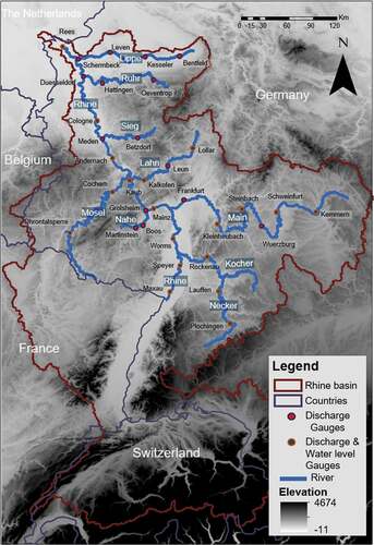
The Rhine River is one of the largest rivers in Europe, with a total length of 1233 km and a total catchment area of 185 260 km² (Fig. 2). It originates in the Swiss Alps and flows through Germany, France, and the Netherlands. Most of Luxembourg and some parts of Austria and Belgium drain into the Rhine River. Major tributaries include Neckar, Main, Moselle, Lahn, Sieg, Lippe, and Ruhr. About 58 million inhabitants live in the river basin, with 10.5 million of them in flood-prone areas (ICPR 2013). The basin topography ranges from high alpine regions with elevations up to 2500 m asl to lowland floodplains of the Lower Rhine. Major floods in the upstream parts of the basin are caused by snowmelt combined with rain-on-snow, whereas the Middle and Lower Rhine floods are dominated by long-lasting frontal rainfalls in winter and early spring. The average discharge at the Lobith gauge at the border between Germany and the Netherlands is 2200 m³/s, and the maximum observed discharge was 12 600 m³/s in 1926 (Pinter et al. 2006). In the past, flood management in the densely populated floodplains was focused on dike reinforcement, with a design discharge corresponding to return periods between 1/200 to 1/500 in Germany and 1/1250 to 1/2000 in the Netherlands (Ministerie van Verkeer en Waterstaat 2006, Te Linde et al. 2011). Consequently, floods may occur in the German parts of the basin, while the Dutch Rhine reaches will likely receive significantly reduced flood flows due to hydrodynamic interactions (Apel et al. 2009).

Figure 2. Rhine basin upstream of Rees with the river network used in the 1D RIM model component. Labelled gauges were used for calibration and validation of the 1D hydrodynamic model.

3.2 Weather generator set-up

The RWG is set up for a large region embracing all of Germany and parts of the neighbouring countries, and covering five major river basins: Ems, Weser, Upper Danube, Elbe, and the Rhine. The set-up is based on daily climate observations for the period 1950–2003. The dataset contains six variables (precipitation; minimum, average, and maximum temperature; relative humidity; and solar radiation) at 528 locations, of which 465 are climate stations (Österle et al. 2016) and 63 are grid points for the French part of the Rhine basin from the E-OBS gridded dataset (Haylock et al. 2008). In this study, we use the RWG to generate 1000 years of synthetic time series for the six mentioned variables, which are then used to drive the SWIM hydrological model.

3.3 SWIM model set-up and calibration

In this study, the Rhine catchment is divided into 936 sub-basins based on the digital elevation data provided by the Federal Agency for Cartography and Geodesy in Germany (BKG). Soil and land-use data are derived from the soil map for Germany (BÜK 1000 N2.3), obtained from Bundesanstalt für Geowissenschaften und Rohstoffe (BGR); from the European Soil Database map, obtained from the European Commission’s Land Management and Natural Hazards unit; and from the CORINE (COoRdinated INformation on the Environment) land-cover map. SWIM is driven by meteorological data, either observations or RWG-generated data. These sub-basins are grouped into eight sub-regions (see Appendix, Fig. A1): Upper Rhine, Nahe, Neckar, Mosel, Lahn, Sieg, Lippe, and Main & Rhine. Nine parameters are automatically calibrated for each sub-region using the SCE-UA optimization algorithm (Duan et al. 1994) (Appendix).

3.4 Set-up and calibration of the RIM 1D model

RIM 1D (both RIM1.0 and RIM2.0) is set up for the river network represented in Fig. 2. The network includes the main channel starting at the Iffezheim weir and major tributaries with a catchment area of at least 500 km². Overbank cross-section geometry is derived from the 10 × 10 m digital elevation model (DEM), with a vertical accuracy of ± 0.5–2 m, provided by BKG.

For the RIM2.0 model, the bankfull depth d_BF is initially estimated using the power-law relationships calibrated on more than 1200 surveyed cross-sections provided by the Federal Institute of Hydrology (BfG) for the Rhine, Mosel, and Necker rivers (Appendix). However, given the uncertainty related to these estimates and the uncertainties of the DEM, we calibrate the estimated bankfull depth in the RIM2.0 model by varying d_BF in the range ± 0.5 m to maximize NSE_m (Equation 7(7) $NS{E}_m=1-\frac{{\sum }_{t}Qobs{\left(Qobs-Qsim\right)}^2}{{\sum }_{t}Qobs{\left(Qobs-Qavg\right)}^2}$(7) ) for the simulated discharge and water level within the calibration period. Bankfull depth calibration was also previously applied by Neal et al. (2012) and Wood et al. (2016). Additionally, the slope used to compute the stage–discharge relation to convert the inflow for each sub-basin into the water level is adjusted in the calibration process to maintain the water balance. The model is manually calibrated based on the period 1996–2003, and the validation is carried out for the whole period between 1 January 1950 and 30 December 1995. Several metrics are considered to assess the performance of the RIM model by comparing the simulated hydrograph by RIM and SWIM models with observed flows at 34 gauging stations and observed water levels at 19 gauges (Fig. 2).

The dike heights represented in the edge points of the cross-section are estimated initially from the 10 × 10 m DEM but are likely to be underestimated due to smoothing effects. Dikes are designed for a specific return period flood (Te Ministerie van Verkeer en Waterstaat 2006, Te Linde et al. 2011). Since no consistent large-scale information on the dike heights is presently available, a regionalized 200-year return period flow in combination with Manning’s equation was used to estimate the elevation of the dikes along the Rhine main channel, while a return period of 100 years was used for other tributaries, according to Te Linde et al. (2011). This step is carried out after the model is calibrated. The estimated dike elevation is compared with the dike levels extracted from the DEM. The higher of the two values is finally taken as a dike crest elevation.

The performance of the model in the calibration and validation periods is evaluated based on the modified Nash-Sutcliffe efficiency NSE_m (Equation 7(7) $NS{E}_m=1-\frac{{\sum }_{t}Qobs{\left(Qobs-Qsim\right)}^2}{{\sum }_{t}Qobs{\left(Qobs-Qavg\right)}^2}$(7) ), which emphasizes peak flows:

(7) $NS{E}_m=1-\frac{{\sum }_{t}Qobs{\left(Qobs-Qsim\right)}^2}{{\sum }_{t}Qobs{\left(Qobs-Qavg\right)}^2}$(7)

where Qobs is the observed discharge at time t, Qsim is the simulated discharge, and Qavg is the mean of observed discharges. Model performance regarding water levels is assessed by mean absolute error (MAE) and mean bias error (MBE), which provide values in metres and thus better guidance on model performance than NSE_m.

3.5 Set-up of the RIM 2D model

The RIM 2D hydrodynamic model is set up on the resampled DEM with a resolution of 100 × 100 m for the areas behind dikes. Floodplains between the dikes or elevated banks are masked in the DEM and are not used for 2D computations. This significantly reduces the computational load. A uniform Manning’s roughness value of 0.03 is assigned to each raster cell, as suggested by Falter et al. (2013), and is not calibrated. The major flood characteristics at this scale are found to be not very sensitive to the floodplain roughness but rather determined by the 1D–2D model interface, and dike heights, i.e. how much water enters the 2D model domain from the 1D model (Bates et al. 2010). Furthermore, no inundation due to dike overtopping occurred in the Rhine basin over the past simulated period, which would allow model calibration.

3.6 Design of computational experiments

To investigate the effect of the hydrodynamic interactions, the RIM2.0 results based on continuous routing are compared to those of RIM1.0. Daily synthetic meteorological data of 1000 years from the regional weather generator are used to drive the SWIM model to generate a set of events exceeding the dike design level. To account for the fact that hydrodynamic models require calibration, which may compensate for the methodological difference between the models, the calibration of the two models is done using the same procedure to make the comparison meaningful and to ensure that the differences between the results of the two models are due to the new conceptual changes. To analyse the effect of hydrodynamic interactions, we compare simulated discharge along the river network. Comparison of overtopping volume resulting in inundation areas and damages elucidates the effect of interactions on hazard and risk. We trace the effects along the channel profile and investigate the role of spatial scale on the effect of hydrodynamic interactions.

4 Results and discussion

4.1 Performance of SWIM, RIM1.0, and RIM2.0 flood routing

In this section, the performance of the hydrological model SWIM and both hydrodynamic models (RIM1.0 and RIM2.0) is presented and discussed. SWIM and RIM2.0 are evaluated in terms of the simulated discharge time series for the period 1950–2003, excluding the calibration period (1996–2003). Further, the simulation of water level hydrographs for RIM2.0 is evaluated. RIM1.0 output cannot be directly compared to SWIM and RIM2.0 output since it routes only overbank flow (flow exceeding bankfull depth) and thus does not produce continuous hydrographs. For this reason, the performance of RIM1.0 is checked visually at the gauge locations, and the ability to reproduce peak flows and water levels is assessed.

Figure 3(a) shows the performance of SWIM over the entire catchment in terms of the NSE_m values. SWIM performance is overall very good, with values ranging from about 0.9 at the Schermbeck gauge (Lower Rhine) down to 0.51 at the Dhrontalsperre gauge on the Mosel River. The latter is likely influenced by the reservoir operation. Further, the performance of RIM2.0 is compared to observed discharge (Fig. 3(b)). Generally, RIM2.0 has a good performance all over the catchment compared to observed hydrographs with NSE_m values ranging from 0.39 to 0.84. However, the performance of RIM2.0 deteriorates compared to SWIM in the downstream parts. We attribute this to the representation of the bankfull depth in the lowland parts of the catchment. Furthermore, floodplains between dikes at the Lower Rhine become much wider compared to upstream parts and are less well represented by the 1D simplified cross-sections. Further improvements in the representation of the cross-section geometry of the downstream reaches are required in the future.

Figure 3. Performance of (a) SWIM and (b) RIM2.0 (NSE_m values) with respect to observed discharges.

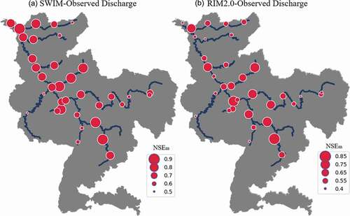
In the Mosel River (Fig. 2), RIM2.0 performs comparably poorly to SWIM, with NSE_m around 0.5, as RIM2.0 is not intended to compensate for errors of preceding modules in the model chain. This is likely a consequence of substantial errors in the precipitation input in the French part of the basin, where coarse-resolution gridded data had to be used. In the Ruhr tributary (Fig. 2) the performance of SWIM is acceptable, with NSE_m between 0.6 and 0.8, whereas RIM2.0 drops below 0.55, likely due to misestimation of river conveyance in this heavily trained reach.

The inspection of the hydrographs for selected flood events, including a major flood in 1993, reveals a very similar performance of RIM1.0 and RIM2.0 at gauges Steinbach, Lauffen, Leun, and Chochem, while SWIM and RIM1.0 slightly better match the observed peak flows compared to RIM2.0 at Cologne and Duesseldorf (see Appendix, Fig. A6). All three models show comparable performance in relation to annual maximum observed flows at most of the selected gauges (see Appendix, Fig. A7). However, RIM2.0 overestimates some high-flow peaks at Lauffen gauge in the Neckar basin and underestimates high-flow peaks in the Lower Rhine. The latter is likely due to an underestimation of bankfull depth, which results in more water conveyed above bankfull depth and stronger attenuated peaks.

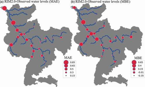
For water level hydrographs, MAE ranges between 0.83 m at Cologne gauge to values below 0.2 m in the Main and Neckar tributaries (Fig. 4), while the MBE ranges between 0.33 m (overestimation) at Lauffen to 0.63 m (underestimation) at Cologne.

Figure 4. Performance of RIM2.0 against observed water level in the validation period. MAE and MBE are calculated as measured minus modelled values. Negative MBE indicates overestimation, and positive MBE indicates underestimation.

Further, we evaluate the performance of RIM1.0 and RIM2.0 with regards to water level simulation at selected gauges in the period December 1993–March 1994, including a major winter flood (see Appendix, Fig. A8), and compare the simulated water levels to observations for annual maximum events (Appendix Fig. A9). RIM2.0 outperforms RIM1.0 in the upstream parts of the Rhine basin and the tributaries. Both models underestimate observed maximum water levels of high-flow events at the Lower Rhine, whereas at Cologne, RIM2.0 underestimation is more severe than that of RIM1.0. A more detailed performance evaluation of all models is provided in the Appendix.

Overall, the models perform reasonably well considering the scale of the basin, the limited information about the cross-section geometry and the degree of anthropogenic influences on river geometry and flow conveyance. The performance of large-scale hydrodynamic models for river networks with uncertain bathymetry reported in the literature is comparable to that achieved in our study. For instance, for the Amazon River and its tributaries, De Paiva et al. (2013) achieved comparable discharge simulation performance with a combined Muskingum-Cunge model and a full St Venant hydrodynamic model, with NSE values mostly between 0.6 and 0.9 but also dropping to 0.2–0.6 for some reaches. Most of the reaches exhibited a bias in the simulated water depths between 3 and 15 m, larger by far than in our study which was in the range of +0.35 to −0.65 m.

4.2 Impact of hydrodynamic interactions on flood hazard

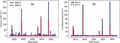
In this section, we analyse the impact of hydrodynamic interactions, which result from inundation and storage effects in the river network, on flood hazard characteristics. First, we compare the overtopping volume over the dike crests and total inundation area in the Rhine basin and present only the results for the first 100 years of the 1000-year simulation period for the sake of brevity (Fig. 5). The tendency is similar for the remainder of the period. Both models show the same major events. RIM1.0 simulates a large number of small events with small inundation areas. In contrast, RIM2.0 simulates overtopping and inundation for only five events in the selected 100-year period. Taking into account the protection level of dikes in the Rhine basin, the overtopping frequency of RIM2.0 appears much more realistic, suggesting that the representation of cross-section geometry, dike height, and water levels is closer to reality in RIM2.0. For the simulated major flood events, the overtopping flow and inundation areas from RIM1.0 are considerably larger than simulated by RIM2.0 (Fig. 5).

Figure 5. (a) Overtopping volume and (b) inundation area simulated by RIM1.0 and RIM2.0 for a 100-year synthetic simulation period. Years in synthetic simulations are denoted with “X.”

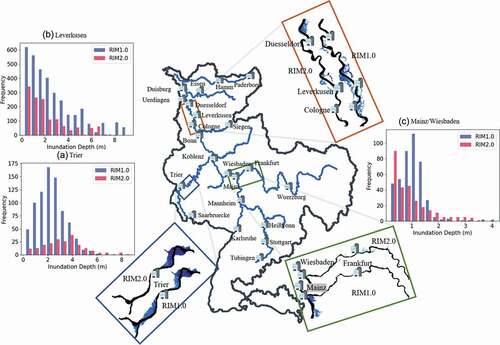
Figure 6 compares inundation areas for the most severe event, Nov-X084, i.e. the event with the highest overtopping volume and inundation area (Fig. 5). The inundation areas tend to occur in the same river reaches; however, RIM1.0 inundations are larger compared to those of RIM2.0. We observe this behaviour for all major events in Fig. 5. Not only inundation areas but also inundation depths are overestimated by RIM1.0, as shown in the histograms of inundation depth for the regions around Trier (Mosel), Leverkusen (Rhine), and Mainz/Wiesbaden (Main).

Figure 6. Comparison of the inundation extent and depth histogram from RIM1.0 and RIM2.0 during the strongest event (Nov-X084) in the first 100-year simulation period. Inundation depths shown for RIM1.0 and RIM2.0 at (a) Trier, (b) Leverkusen, and (c) Mainz/Wiesbaden for the Nov-X084 event.

These results suggest that the hydrodynamic interactions, which are insufficiently represented in RIM1.0, considerably reduce water levels downstream. This is further illustrated by analysing the longitudinal profiles of maximum water level and overtopping volume for the Moselle River and the Rhine during the Nov X084 and April X068 events (Fig. 7). The profiles start at the upstream node in the Moselle River and continue along the Middle and Lower Rhine. We select this course since inundation mainly occurs along these tributaries in these two events.

Figure 7. Longitudinal profile of the maximum water level (left y-axis), the difference in maximum water level between RIM1.0 and RIM2.0 (right y-axis), and the overtopping locations represented by points of different sizes corresponding to the overtopping volume in million m³. The profile corresponds to events Nov X084 and April X068 from the Moselle River to Rees at the outlet of the Rhine catchment. Confluences of major tributaries such as Saar, Rhine, Sieg, Ruhr, and Lippe are indicated with vertical dashed lines.

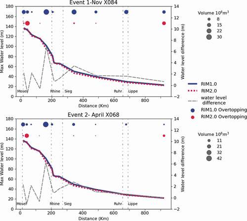
Figure 7 shows that the difference in maximum water levels between RIM1.0 and RIM2.0 fluctuates around zero at the upstream part of Mosel and is controlled by overtopping in both models. The maximum difference happens upstream of the confluence with the Rhine River at Trier (see Fig. 2), which results in the highest overtopping (spatially during both events), and consequently the greatest difference in inundation depth and extent (Fig. 6) between the two models. The overtopping frequency and volume are noticeably higher in RIM1.0 at the downstream reaches compared to RIM2.0 for both events. The maximum water levels in RIM1.0 are much less sensitive to overtopping compared to RIM2.0. In consequence, RIM1.0 produces a higher overtopping volume along the entire reach. We explain this pattern by the hydrodynamic interactions. RIM1.0 considers hydrodynamic interactions only within individual sub-basins, i.e. dike overtopping and inundation cause discharge and water level reductions only within the sub-basin where they occur. This storage effect is not translated to the sub-basin downstream. The discharge boundary condition in the subsequent sub-basin is updated using SWIM output, which is not aware of the overtoppings upstream. Hence, the total floodwater volume in the river system is overestimated, causing stronger overtopping and larger inundation areas in RIM1.0.

To some extent, this effect also occurs in the mosaic flood mapping approach, in which upstream boundary conditions of piece-wise hydrodynamic models are updated from the local regionalized flood frequency curves (e.g. Quinn et al. 2019). There may be cases where the streamflow observations comprise events with upstream inundations and, thus, downstream flow reductions, which then may leave a trace in the flood frequency curve. However, given the length of measured discharge series and the rarity of dike overtopping and inundations along embanked rivers, the degree to which the effect of hydrodynamic interactions is contained in the results of the extreme value statistics is limited.

4.3 Impact of hydrodynamic interactions on damage and risk

In this section, we investigate how decisive hydrodynamic interactions are for flood damage and risk estimates. For this, we integrate the risk from all flood events simulated in the 1000-year period of synthetic simulations. The comparison of estimated economic risk from the two models (Fig. 8) indicates that the chain, including RIM2.0, generally simulates less damage. This corresponds to the overall smaller inundation areas and depths discussed in the previous section. We attribute this difference in particular to the effect of hydrodynamic interactions. We analyse the overall simulated damages and flood risk in the Rhine basin and discuss the results in view of previous studies.

Figure 8. Risk per economic sector derived from both model chains; the VAR and TVAR and the EAD values are displayed for the two models, in blue (RIM1.0) and red (RIM2.0), respectively. The agriculture loss is given in € millions, in contrast to other sectors.

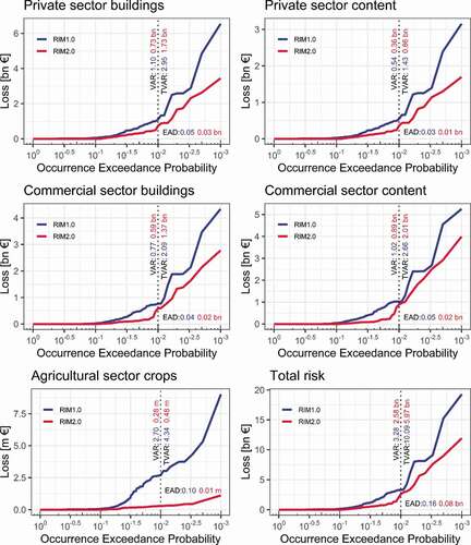
Simulated absolute damage numbers for the residential, commercial, and agricultural sectors are in reasonable agreement with actual reported losses, though a direct comparison between single observed and simulated events is not expedient. For instance, VAR, i.e. the 100-year total loss, amounts to 1.94 billion € in RIM2.0 compared to 3.14 billion € in RIM1.0, while the reported loss of the 1993 event (about a 100-year flood at Cologne) in the German Rhine was 1.5 billion DM (Engel 1997), which corresponds to roughly 1.2 billion € today. The estimated EAD for the two model variants (0.16 billion € by RIM1.0 and 0.08 billion € by RIM2.0) is considerably lower than that estimated by Te Linde et al. (2011) (0.79 billion € for the German Rhine). This difference likely originates from the differences in the approaches used to compute flood hazard, asset values and different damage models. First, the approach of Te Linde et al. (2011) is based on the homogeneous assumption of an “extreme” inundation scenario provided by ICPR (2005) without an associated return period. Probabilities of inundation and losses in that study were retrospectively assigned using the nominal protection levels in the respective parts of the Rhine reach. Hence, EAD was estimated as summed probability-weighted losses corresponding to the return period of dike overtopping, i.e. dike design level. Damage estimations corresponding to a specific high return period under homogeneous assumptions are found to be largely overestimated (Metin et al. 2020). Second, the exposure values used in the Damage Scanner model in Te Linde et al. (2011) include infrastructure and other land-use types not considered in our approach. Damage Scanner is found to overestimate loss values by more than three times compared to the FLEMO damage model (Jongman et al. 2012). Finally, damage calculated by Te Linde et al. (2011) comprises a share of, on average, 5% indirect damage, which is not accounted for in our study.

The private and commercial sectors contribute equally to the overall financial risk in our simulation. However, the loss in the agricultural sector differs greatly between the two models due to the difference in the inundation extent; it only accounts for a small fraction of the overall loss (Fig. 8). This result is expected for the highly industrialized Rhine catchment, particularly the Lower Rhine. The difference in TVAR is larger than the difference in VAR, indicating that the models show less agreement in the upper tail. We find that events above the 100-year return period contribute significantly to the difference in risk curves between the RIM1.0 and RIM2.0 model chains. Different protection levels around 100- and 200-year return periods can be observed in the loss curves. A steep growth of the curve is visible at these thresholds, depending on whether damages occur along the main course with the higher protection standard (~200 years) or in the tributaries, where the protection standard is likely lower (~100 years).

OEP considers the most severe event per year. However, there is a possibility of having multiple flood events in one year, which can then be reflected in the risk curves by the aggregated exceedance probability (AEP). As the AEP and OEP values are mostly identical (not shown), which means that both models (RIM1.0 and RIM2.0) seldom encounter two major events per year, only OEP values are presented.

To analyse the impact of hydrodynamic interactions on flood damage and risk, we sub-divide the river network into different segments based on the location of major cities and confluences (Fig. 9). The results of both RIM1.0 and RIM2.0 are aggregated and used to derive the risk curves for each segment. At the upstream segments 1, 7, and partially 10, the risk curves by RIM2.0 are higher than those of the RIM1.0 curves, which indicates higher losses produced by RIM2.0. Farther downstream, the risk curves converge (segments 2 and 3). At the lower part of the Rhine (segments 4, 5, and 6), the risk modelled by RIM1.0 consistently exceeds the estimations by RIM2.0. In these segments with extended floodplains and high exposure, there is a strong potential for widespread inundation and high losses. In segment 9, i.e. the Lippe tributary, the RIM2.0 calibration results with respect to discharge are poor (Fig. 3), presumably due to anthropogenic effects on river geometry and discharge in this strongly affected reach. Moreover, water levels were not available for model calibration, which affects water level estimations. Hence, significant differences resulted between RIM1.0 and RIM2.0 in this reach that explain the resulting risk curves. The discharge contribution of this segment to the main Rhine channel is on the order of a few percent, so the effect on the risk downstream is expected to be small.

Figure 9. Risk curves derived from RIM1.0 and RIM2.0 for river basin segments at different locations across the main Rhine and the tributaries.

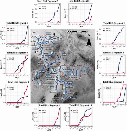
Figure 10. Comparison of inundation area and damage between RIM1.0 and RIM2.0 for two selected events in the synthetic series. The shaded colour in the background refers to the maximum inundation area of both models in the left panels, and the maximum damage of both models in the right panels, for the same sub-area. The bars indicate the share (%) of each model from the maximum value of the sub-area, i.e. one of the two bars refers to 100% in each sub-area.

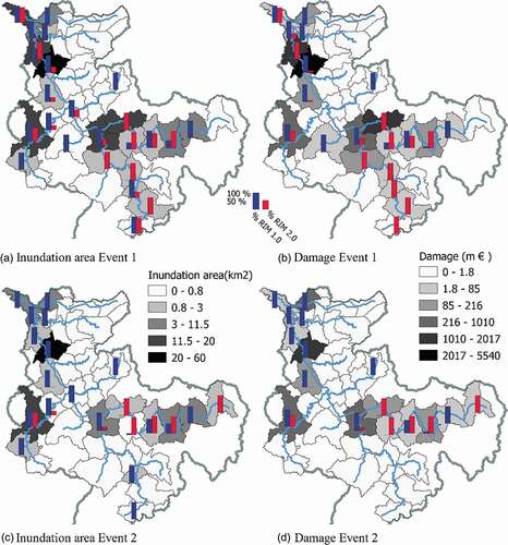
Figure 10 compares the spatial distribution of inundation areas and damages for two large events (Nov-X084 and April-X068; see Fig. 5). The inundation areas and damages are aggregated for the sub-areas shown in Fig. 10. To present the results on a proper scale, the hydrological sub-basins of SWIM are aggregated to larger areas. The total damage of the Nov-X084 event is 7.9 billion estimated from RIM1.0 and 5.6 billion from RIM2.0, while the April-X068 event simulation results in 3.2 billion and 1.0 billion for RIM1.0 and RIM2.0, respectively. Locating these numbers on the risk curves would result in return periods of 200 and 166 years for the Nov-X084 event simulated by RIM1.0 and RIM2.0, respectively, and 100 and 66 years for the April-X068 event by RIM1.0 and RIM2.0, respectively. The shading of the sub-area indicates the absolute inundation area/damage. Nov-X084 event originates in the Neckar, Main, and Mosel tributaries, whereas the April-X068 event strikes Main and Mosel (see Fig. 2 for orientation), and the Lower Rhine is affected by both floods. For both events, inundation areas and damage simulated by RIM1.0 are often similar at upstream sub-areas but clearly dominate the Lower Rhine compared to the RIM2.0 results. The Lower Rhine is hardly affected by Event 2 in the RIM2.0 model.

We attribute the difference in inundation/damage patterns between the two models mainly to the difference in the routing scheme and, consequently, to the consideration of hydrodynamic interactions. However, underestimation of flow and water level in RIM2.0 compared to RIM1.0 due to differences in cross-section geometry and parameterization may result in less inundation in RIM2.0 and thus represents a limitation for the achieved results. The higher sensitivity of RIM2.0 simulations to dike overtopping due to the consideration of hydrodynamic interactions becomes pronounced in the Lower Rhine, where several overtoppings occur during these events. Consequently, less inundation and damage occur during both events at the Lower Rhine, when hydrodynamic interactions are accounted for.

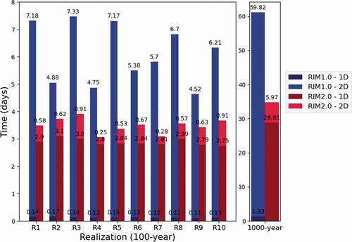
4.4 Computational time performance

Besides considering hydrodynamic interactions and a more plausible representation of dike overtopping events leading to inundation, we achieve a considerable reduction of the computational time with RIM2.0. The model runtime for the 1000-year simulation run was nearly halved (from about 60 to 30 days on the GPU cluster – NVIDIA Tesla K80 with 24 GB of GDDR5 RAM). The computational load in RIM2.0 caused by the 1D component increased nearly 20-fold compared to RIM1.0. 1D routing in RIM2.0 runs continuously for all flows, whereas RIM1.0 routes only flow exceeding the 2-year discharge. This happens every second year on average. However, due to the lack of hydrodynamic interactions in RIM1.0, the overall larger inundation computations result in a much longer 2D computational time (see Appendix, Fig. A10).

5 Conclusions

In this work, we analyse the effects of hydrodynamic interactions on flood hazard and risk estimates. To this end, two versions of the 1D–2D coupled hydrodynamic diffusive wave models driven by a weather generator and a hydrological catchment model were compared – RIM2.0 considering hydrodynamic interactions, and RIM1.0 considering interactions only within individual sub-basins or river reaches, but not beyond sub-basin boundaries.

The analysis of peak water levels, overtopping volumes, and inundation areas and depths reveals that the piece-wise routing approach is largely insensitive to overtopping. Unconsidered hydrodynamic interactions and updated upstream boundary conditions at each sub-basin from the hydrological model largely contribute to this effect. The hydrological model is unaware of upstream inundations and provides hydrologically routed flow, including lateral input, as if no upstream overtopping has occurred. In this way, the overall mass balance is violated in the piece-wise routing approach and leads to larger inundation areas, depths, and damages. At some reaches this overestimation is, however, partly caused by differences in simulated discharges between two models resulting from calibration and uncertainties in cross-section geometry. We conclude that considerable risk overestimation can be expected when using mosaicking of piece-wise hydrodynamic simulations driven by hydrological models or extreme value statistics as an upstream boundary condition. This approach is still very commonly used for fluvial flood risk assessments.

Even if extreme value statistics account for multisite spatial dependence structure, hydrodynamic interactions are only accounted for along the reach considered in the hydrodynamic model. Our results for the Rhine basin suggest that the interaction-aware model produces smaller inundation areas and hence requires half of the computational time for the 2D component compared to the piece-wise approach. The overall risk estimates, i.e. the EAD, derived by the RIM2.0 model version are just about half the values provided by RIM1.0. This highlights the practical relevance of the continuous routing considering hydrodynamic interactions for large-scale flood risk analysis.

Author contributions

SV, KDB, and BM conceptualized the study. MF developed the 1D hydrodynamic code and calibrated both RIM1.0 and RIM2.0 models, carried out 1D–2D model simulations, run the SWIM model, and, together with SV, analysed the results and drafted the initial manuscript. DVN run the weather generator, calibrated the SWIM model, and contributed to the analysis of the results. NS estimated exposure values, and FB carried out damage and risk assessment supervised by KS and HK. All authors contributed to the final manuscript.

Acknowledgements

We acknowledge funding received from the European Union’s Horizon 2020 research and innovation programme under the Marie Skłodowska-Curie Grant. This work contributes to the DFG Research Unit FOR 2416 “Space-Time Dynamics of Extreme Floods (SPATE).”

Disclosure statement

No potential conflict of interest was reported by the authors.

Data availability statement

The hydrometric data used in this paper were provided by the German water management authorities and are not publicly accessible. The authors can be contacted ([email protected], [email protected], [email protected]) with inquiries about the data.

Additional information

Funding

This work was supported by the Marie Sklodowska-Curie Grant [grant agreement 676027].

Appendix

1 Calibration of the hydrological model SWIM

SWIM has a set of nine most sensitive parameters which need to be estimated. Two parameters are related to the channel routing, three parameters pertain to snowfall and snowmelt processes, two parameters control the subsurface flow contribution to the streamflow, and there is a correction parameter for potential evaporation and a correction parameter for saturated conductivity. SWIM is calibrated in two phases. In the first phase, we calibrate and validate the model for all sub-regions, except Main & Rhine, independently (Fig. A1). In the second phase, the Main & Rhine sub-region is calibrated and validated. It uses the input from other already calibrated sub-regions as tributary inflow. Observed daily streamflow at 79 selected stations is used to calibrate the model based on the modified Nash-Sutcliffe Efficiency, NSE_m (Equation 7(7) $NS{E}_m=1-\frac{{\sum }_{t}Qobs{\left(Qobs-Qsim\right)}^2}{{\sum }_{t}Qobs{\left(Qobs-Qavg\right)}^2}$(7) ). The period between 1 January 1981 and 31 December 1989 is used for the calibration, while the period between 1 January 1950 and 3 December 2003 is considered for validation (excluding the calibration period).

2 Description of the RIM1.0 and RIM2.0 hydrodynamic model discretization and cross-section geometry

2.1 Discretization and coupling to the hydrological model SWIM

The discretization depends mainly on the river topography and SWIM model sub-basins. Each cross-section in the 1D model is linked to a specific SWIM sub-basin, whereby several cross-sections can be linked to one sub-basin. There can also be sub-basins that contain no cross-sections, i.e. no river channels are discretized within these sub-basins (Fig. A2). In the latter case, the flow between sub-basins is routed by SWIM using the Muskingum routing method. For RIM1.0, at the upstream point of each sub-basin, the 2-year return period discharge is first subtracted from the SWIM flow hydrographs (explicitly representing the bankfull depth), then used as a boundary condition for the RIM 1D component. For RIM2.0 the flow hydrographs are used as upstream boundary conditions at the most upstream nodes of the discretized river network. Otherwise, the sub-basin discharge is distributed as lateral inflow at every time step among the cross-sections linked to a specific sub-basin.

2.2 River cross-section data

2.2.1 Overbank cross-section area

The 1D hydrodynamic model (both RIM1.0 and RIM2.0) requires river cross-section data to describe the river channel geometry. In our approach, the entire river channel and adjacent overbank areas between the dikes or elevated banks are characterized by the river cross-sections and represented in the 1D model domain. Surveyed cross-sections are often not available for large river networks. Furthermore, they usually do not cover the entire floodplain between dikes as represented in the RIM approach. Therefore, RIM relies on cross-sections derived from a digital elevation model (DEM). However, the bankfull depth, i.e. river bathymetry below the water level, is not represented in the DEM. The cross-sections for the RIM1.0 are directly extracted from the DEM. For the RIM2.0 model, we additionally estimate the bankfull depth using three options based on power-law functions that are detailed below.

First, the overbank component of the river cross-sections, including dike location and elevation along the river network, is derived from the DEM perpendicular to the flow direction, with the GIS integrated tool HEC-GeoRas. Additional information on dike locations and channel width can be taken from the digital basic landscape model (Base DLM). Subsequently, cross-sections were simplified into six-point cross-sections by retaining the cross-sectional area (Appendix, Fig. A2) using an optimization procedure, i.e. a point is varied vertically on each floodplain side until the optimized vertical location of those points corresponds to the minimal difference between the resulting area and original cross-section area (Appendix Fig. A3(a)). Typically, low-resolution DEMs do not resolve dike heights well and tend to underestimate them. Therefore, dike height derived from the DEM is further calibrated based on a design flow return period. The highest of both estimates is adopted as a crest height in the cross-sections.

2.2.2 Cross-section bankfull depth in RIM2.0

The bankfull depth for all cross-sections in the RIM2.0 model is derived using hydraulic geometry relationships (Leopold 1953). Three different approaches to derive bankfull depth based on the power-law functions (Equations A1–A4) can be used to estimate the bankfull depth at each derived cross-section from the DEM. The first one relates bankfull depth to the 2-year discharge:

(A1) $d_{BF}=a\hspace{0.17em}H{Q_2}^b$(A1)

(A2) $W_{BF}=c\hspace{0.17em}H{Q_2}^d$(A2)

where $W_{BF}$ is the bankfull width (m), $d_{BF}$ is the mean bankfull depth(m), and HQ₂ is the 2-year discharge (m³ s⁻¹). Based on Rawlins (1994), flows corresponding to 1–2.5 years are representative of bankfull discharge for stable natural channels; therefore, the two-year return period discharge (HQ₂) is calculated for all locations with observed discharge by fitting the Gumbel distribution to the annual maximum discharge series at the observational gauges. Since the value of HQ₂ is required at all cross-section locations along the river, not only at gauges, we fit the power-law curve $H{Q}_2=\alpha \hspace{0.17em}{A}^{\beta }$, where A is the upstream drainage area (m²), to the data via regression and use this curve to estimate HQ₂ at all cross-sections.

To estimate the target variable d_BF, coefficients a and b need to be approximated. Using Manning’s equation, we obtain the bankfull depth (d_BF). The bankfull width W_BF and slope S₀ are estimated from the DEM. Based on the estimated d_BF with the very wide cross-sections, the a and b parameters in Equation (A1.1) are obtained by the regression analysis. Using Equation (A1), the bankfull depths can directly be derived.

Furthermore, the relationship between channel width and 2-year discharge (Equation A2) was derived through regression analysis to get the parameters c and d; this relationship is not used to calculate the bankfull width as it is extracted from the DEM for all cross-sections, therefore the role of the relationship in Equation (A2) is to obtain the parameters c and d and use them in Equations (3)(3) $\frac{\mathrm{\partial }{Q}_{bf}}{\mathrm{\partial }x}+\frac{\mathrm{\partial }{A}_{bf}}{\mathrm{\partial }t}+\frac{\mathrm{\partial }{Q}_{Overbank}}{\mathrm{\partial }x}+\frac{\mathrm{\partial }{A}_{Overbank}}{\mathrm{\partial }t}=0$(3) and (4(4) $q_{t+\mathrm{\Delta }t}=\frac{q_t-g{h}_{flow}\mathrm{\Delta }t{S}_f}{\left(1+g{h}_{flow}\mathrm{\Delta }t{n^2}_{\left|q_t\right|}{/}_{h_{flow}}\frac{10}{3}\right)}$(4) ).

By multiplying Equations (A1) and (A2), another relationship based on the two predictors W_BF and HQ₂ can be obtained (Equation A3). Then the third option to derive d_BF is to substitute HQ₂ from Equations (A1) into Equation (A2), resulting in Equation (A4):

(A3) $d_{BF}=\frac{ac}{W_{BF}}\hspace{0.17em}H{Q_2}^{b+d}$(A3)

(A4) $d_{BF}=a\hspace{0.17em}\left(\frac{W_{BF}}{c}\right){\hspace{0.17em}}^{b/d}$(A4)

The bankfull depths derived using three approaches are assessed against the bankfull depths of the surveyed cross-sections at about 1100 locations along the Rhine, Mosel, and Neckar using mean absolute error (MAE) and the mean bias error (MBE). Different Manning’s roughness values between 0.025 and 0.05 are considered to estimate the value of d_BF, but the differences are found to be non-significant. Ultimately, the uniform value of n = 0.03 is used across the river network. Considering different options to derive bankfull depth, Equation (A5) is found to deliver the best fit, with an overall MAE of 1.01 m and MBE of 0.12 m (Fig. A4). It used measured bankfull width from the DEM as a single predictor. The error in the calculated bankfull depth in the Rhine main channel (MAE of 1.02 and MBE of −0.37) differs slightly from that of the Mosel (MAE of 1.03 and MBE of 0.46) and Neckar (MAE of 0.99 and MBE of 0.63) tributaries.

(A5) $d_{BF}=0.6354\hspace{0.17em}\left(\frac{W_{BF}}{0.7093}\right){\hspace{0.17em}}^{0.3961}$(A5)

Figure A4 shows considerable variability in the estimation of bankfull depth used in RIM2.0 for single cross-sections compared to observations. This highlights the need to calibrate the model by adapting the bankfull depth to match the water level and discharge hydrographs.

To analyse the effect the cross-section estimation method has on the calculation of bankfull capacity and thus on flow and water level, we compare the bankfull capacity of the cross-sections in RIM1.0 and RIM2.0 at the locations of the gauging stations with the estimates of the 2-year flood based on the gauge records (Fig. A5). The bankfull discharge (cut-off value) in RIM1.0 is estimated for each sub-basin based on the simulated flows with the SWIM hydrological model. For the purpose of this comparison, the bankfull discharge of RIM2.0 cross-sections is estimated with Manning’s equation. The basin average bankfull discharge is then compared to the respective gauge-based estimations. Figure A5 shows the difference between the observations and both model estimations. At most locations, the bankfull discharge in the RIM2.0 model (red) marginally differs from the observed two-year discharge, which indicates a sound estimation of the bankfull depth and conveyance. Only in the upstream parts of the Neckar and the Nahe tributary is the bankfull conveyance considerably overestimated. The RIM1.0 tends to slightly overestimate the observed two-year discharge in the downstream part of the Rhine and in the main tributary.

3 Performance of SWIM, RIM1.0, and RIM2.0 flood routing

3.1 Performance of discharge simulation

Figure A6 presents a comparison of a few selected flood events exceeding 2-year bankfull discharge in the observation period at six gauges (for the locations of gauges see Fig. 2) in the Rhine basin, including the comparison with RIM1.0, where the cut-off value is represented by the horizontal dotted blue line. These peaks belong to a major flood event which hit the Rhine catchment in December 1993–January 1994. These gauges are selected to cover the main channel and major tributaries, including potential risk hot spots at the Lower Rhine (Cologne, Duesseldorf). An inspection of the hydrographs in Fig. A6 reveals a very close performance of the two model versions at the Steinbach, Lauffen, and Leun and Cochem gauges, while the performance at Cologne and Duesseldorf slightly differs, where SWIM and RIM1.0 better match the observed peak flows.

The comparison of the modelled and observed hydrographs reveals that the performance of the RIM models with respect to observations is affected by the input from SWIM. For example, at gauge Leun, SWIM underestimates the peak flows, and this error inherently appears in the RIM results. In general, the comparison reveals that RIM2.0 mostly captures the peak magnitudes, but shows a slight shift in phase of the hydrographs at nearly all gauges. The peaks come earlier and appear to be less attenuated than in other models, and this explains the poorer performance compared to SWIM routing. The performance of RIM2.0 compared to observations tends to be worse compared to the performance of the SWIM routing. This might be due to the fact that the calibration of the cross-section bankfull depth changes the bed slope between cross-sections. This controls the water levels and, consequently, discharge calculations. Hence, a certain trade-off is expected in the performance with respect to the water levels vs the discharge hydrographs. In other words, the performance with respect to discharge can deteriorate compared to SWIM in order to improve the simulation of water levels.

Figure A7 presents a comparison of the maximum annual discharges in the validation period modelled by RIM1.0, RIM2.0, and SWIM vs the observed peak flow of the corresponding flood events. It can be noticed that RIM1.0 does not simulate flows below the HQ₂ threshold. Therefore, the number of peaks simulated by the RIM1.0 is roughly half the number of those delivered by the other two models. The points for all models are scattered along the 45-degree line at most of the selected gauges, which indicates an overall similar model performance with regards to peak flows. At gauge Steinbach, RIM1.0, RIM2.0, and SWIM perform very similarly but slightly overestimate the peaks. At Lauffen, RIM2.0 overestimates a few high-flow peaks. At gauges Duesseldorf and Cologne, RIM2.0 slightly underestimates the peaks above 8000 m³/s, whereas RIM1.0 and SWIM show very good performance. As discussed above, the representation of the cross-sectional geometry in the lowland river reaches might be inadequate and requires further improvement in future.

3.2 Evaluation of RIM1.0 and RIM2.0 with regards to water levels

To benchmark the performance of RIM1.0 and RIM2.0, we analyse the water level simulations at six selected gauges with available water level observations for the major flood event in 1993 analogously to the analysis of discharge hydrographs (Fig. A8). RIM1.0 and RIM2.0 are mostly consistent in the simulation of water level dynamics and match the peak levels similarly well (or poorly). As for discharge, RIM2.0 water level hydrographs are slightly shifted in time compared to RIM1.0 and observed hydrographs, though peak levels are mostly well matched. The constant water level in RIM1.0 (horizontal line) is the water level corresponding to the cut-off value (HQ₂). At the Speyer gauge station, water levels simulated by RIM2.0 show that both high and low flows are well presented in addition to the timing of the flood wave, with 0.48 m MAE and −0.05 m MBE (overestimation). In contrast, RIM1.0 misses the event, which indicates a problem in RIM1.0 for estimation bankfull capacity. At the Andernach gauge, both models predict a slightly earlier peak compared to the observed data, but RIM2.0 matches the observed peak water levels much better than RIM1.0 At the Cologne and Rees gauges, RIM2.0 simulates slightly lower water levels than RIM1.0 for some peaks, whereas other peaks are well attained by RIM2.0 and are entirely missed by the RIM1.0 model. At the Cochem gauge RIM2.0 underestimates the peaks, with MBE of 0.19 and MAE of 0.46. The degradation of the water level performance at Cochem indicates a problem in the bankfull depth estimation at the cross-sections in this reach and should be revised in future. The Steinbach gauge in the middle of the river Main shows that RIM1.0 underestimates smaller events, while RIM2.0 manages to capture the observed peaks and delivers a good performance, with MBE of −0.08 m and MAE of 0.28 m.

Figure A9 presents a comparison between the water levels modelled by RIM1.0 and RIM2.0 for flood events corresponding to events with the maximum annual observed water level peaks. Similar to the simulated discharge by RIM1.0 and RIM2.0, the simulated water levels of both models have an overall similar model performance but are underestimated at most stations, as shown in Fig. A9. RIM2.0 seems to have problems replicating the peak water levels at Cologne. Nonetheless, the performance of the two models is very similar at Duesseldorf (not shown). This highlights the effect of the cross-sections on water levels estimates and stresses the importance of the robust estimation of the river profile geometry.

3.3 Computational time performance

See Fig. A10.

Figure A1. SWIM model set-up with eight calibration sub-regions, each sharing the same parameter values. The river network shown is the result of the catchment delineation and is used in SWIM. It differs from the river network used in RIM (Fig. 2).

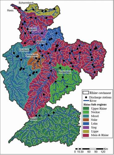
Figure A2. Difference between the (a) piece-wise routing and (b) continuous routing approaches considered in RIM1.0 and RIM2.0, respectively. Computational nodes are imaginary points at which discharge and water levels are computed. The calculation at points with the notation “Flow (#)” refers to the addition of the upstream flow, while calculation with the notation “*#” refers to routing using the diffusive wave approximation.

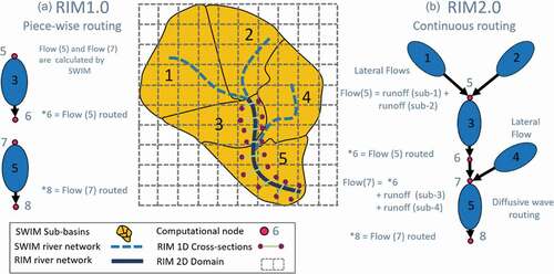
Figure A3. Difference between cross-section shapes considered in the two model versions (a) RIM1.0 and (b) RIM2.0. The overbank area is represented by a six-point cross-section derived from the 10 × 10 m DEM for both models. In RIM1.0, the bankfull area is represented by two-year flow, while in RIM2.0, it is derived statistically from hydraulic geometry relationships.

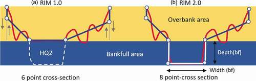
Figure A4. Comparison of estimated and measured bankfull depth at the locations of the surveyed cross-sections; MAE and MBE are calculated as measured value minus calculated value.

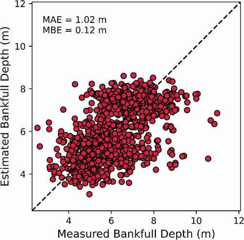
Figure A5. Comparison between the two-year return period discharge derived from gauge observations (grey column), cut-off value (HQ2) in RIM1.0 (blue column), and estimated bankfull cross-section capacity in RIM2.0 (red column) in m³/sec. The bar height is related to the maximum value at each location. Bars at one location cannot be compared with those at other locations.

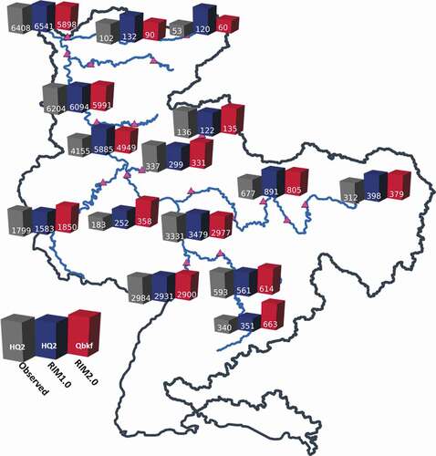
Figure A6. Comparison of discharge hydrographs between RIM1.0, RIM2.0, SWIM, and observations at selected gauges. The selected dates show the highest peak of the time series in the observational period. The horizontal blue line represents the cut-off value (HQ₂) in RIM1.0 and is not simulated.

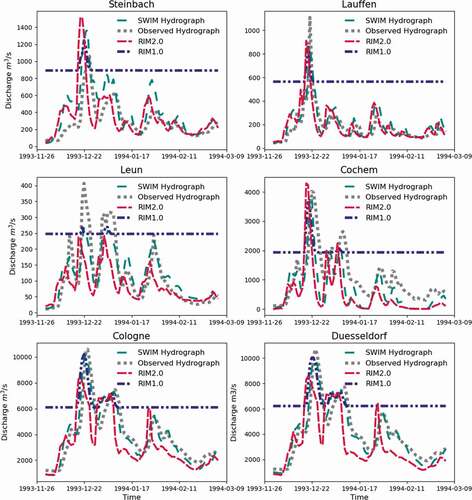
Figure A7. Comparison of the maximum annual modelled and observed discharge peaks in the historical period from 1950 to 2003.

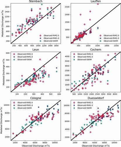
Figure A8. Comparison of water levels simulated by RIM1.0 and RIM2.0 for selected historical flood events in the period December 1993–January 1994 at six selected gauges.

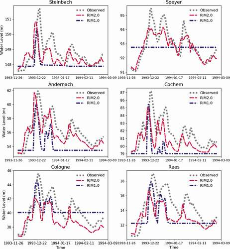
Figure A9. Comparison of the maximum annual modelled and observed highest water level in the historical period from 1950 to 2003.

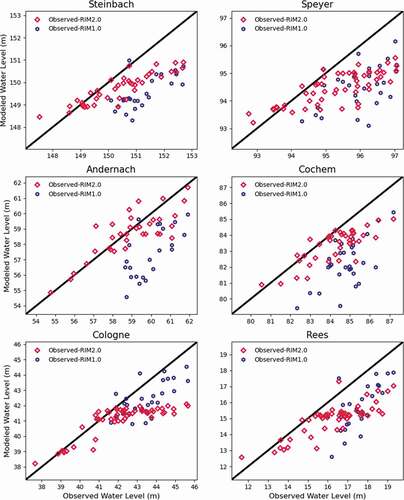
Figure A10. Computational time required by RIM1.0 and RIM2.0 for simulating 1000 years. The 1000-year period is divided into 10 realizations, each modelled using one NVIDIA Tesla K80 card.

References

- Alfieri, L., et al., 2014. Advances in pan-European flood hazard mapping. Hydrological Processes, 28 (13), 4067–4077. doi:https://doi.org/10.1002/hyp.9947
- Alfieri, L. et al., 2016. Modelling the socio-economic impact of river floods in Europe. Nat. Hazards Earth Syst. Sci, 16 (6), 1401–1411. doi:https://doi.org/10.5194/nhess-16-1401-2016
- Apel, H., et al., 2004. Flood risk assessment and associated uncertainty. Natural Hazards and Earth System Sciences, 81 (2), 343–347. doi:https://doi.org/10.5194/nhess-9-289-2009
- Apel, H., Merz, B., and Thieken, A.H., 2009. Influence of dike breaches on flood frequency estimation. Computers & Geosciences, 35 (5), 907–923. Elsevier. doi:https://doi.org/10.1016/j.cageo.2007.11.003
- Bates, P.D., Horritt, M.S., and Fewtrell, T.J., 2010. A simple inertial formulation of the shallow water equations for efficient two-dimensional flood inundation modelling. Journal of Hydrology, 387, 33–45. doi:https://doi.org/10.1016/j.jhydrol.2010.03.027
- Biancamaria, S. et al. 2009. Large-Scale coupled hydrologic and hydraulic modelling of the Ob river in Siberia. J. Hydrol Vol. 379(1–2), pp. 136–150. Elsevier. doi:https://doi.org/10.1016/J.JHYDROL.2009.09.054
- Blazkova, S. and Beven, K. 2004. Flood frequency estimation by continuous simulation of subcatchment rainfalls and discharges with the aim of improving dam safety assessment in a large basin in the Czech Republic. J. Hydrol Vol. 292(1–4), pp. 153–172. Elsevier. doi:https://doi.org/10.1016/J.JHYDROL.2003.12.025
- Bradbrook, K., Waller, S., and Morris, D., 2005. National floodplain mapping: datasets and methods – 160,000 km in 12 months. Natural Hazards, 36 (1–2), 103–123. doi:https://doi.org/10.1007/s11069-004-4544-9
- Ciullo, A. et al., 2019. Accounting for the uncertain effects of hydraulic interactions in optimising embankments heights: Proof of principle for the IJssel River. J. Flood Risk Manag, 12 (January), 1–15. doi:https://doi.org/10.1111/jfr3.12532
- Cunge, J.A., 1969. On the subject of a flood propagation computation method (Muskingum method). Journal of Hydraulic Research, 7 (2), 205–230. doi:https://doi.org/10.1080/00221686909500264
- Curran, A., et al., 2019. Large scale flood hazard analysis by including defence failures on the Dutch River System. Water, 11 (8), 1732. doi:https://doi.org/10.3390/w11081732
- Curran, A. et al. 2020. Large-Scale stochastic flood hazard analysis applied to the Po River. Nat. Hazards Vol. 104 (3), pp. 2027–2049. Springer Netherlands. doi:https://doi.org/10.1007/s11069-020-04260-w
- de Bruijn, K.M., Diermanse, F.L.M., and Beckers, J.V.L., 2014. An advanced method for flood risk analysis in river deltas, applied to societal flood fatality risk in the Netherlands. Natural Hazards and Earth System Sciences, 14 (10), 2767–2781. doi:https://doi.org/10.5194/nhess-14-2767-2014
- de Moel, H., et al., 2015. Flood risk assessments at different spatial scales. Mitigation and Adaptation Strategies for Global Change, 20 (6), 865–890. doi:https://doi.org/10.1007/s11027-015-9654-z
- De Paiva, R.C.D., et al., 2013. Large-scale hydrologic and hydrodynamic modeling of the Amazon River basin. Water Resources Research, 49 (3), 1226–1243. doi:https://doi.org/10.1002/wrcr.20067
- Duan, Q., Sorooshian, S., and Gupta, V.K., 1994. Optimal use of the SCE-UA global optimisation method for calibrating watershed models. Journal of Hydrology, 158 (3–4), 265–284. doi:https://doi.org/10.1016/0022-1694(94)90057-4
- Dupuits, E., et al., 2019. Impact of including interdependencies between multiple riverine flood defences on the economically optimal flood safety levels. Reliability Engineering & System Safety, 191, 106475. doi:https://doi.org/10.1016/J.RESS.2019.04.028
- Engel, H., 1997. The flood events of 1993/1994 and 1995 in the Rhine River basin. IAHS-AISH Publication, 239, 21–32.
- Falter, D., et al., 2015. Spatially coherent flood risk assessment based on long-term continuous simulation with a coupled model chain. Journal of Hydrology, 524, 182–193. Elsevier B.V. doi:https://doi.org/10.1016/j.jhydrol.2015.02.021
- Falter, D., et al., 2016. Continuous, large-scale simulation model for flood risk assessments: proof-of-concept. Journal of Flood Risk Management, 9 (1), 3–21. doi:https://doi.org/10.1111/jfr3.12105
- Falter, D. et al., 2013. Hydraulic model evaluation for large-scale flood risk assessments. Hydrological Processes, 27 (9), 1331–1340. doi:https://doi.org/10.1002/hyp.9553
- Fleischmann, A., et al., 2019. Modeling the role of reservoirs versus floodplains on large scale river hydrodynamics. Natural Hazards, 99 (2), 1075–1104. Springer Netherlands. doi:https://doi.org/10.1007/s11069-019-03797-9
- Fread, D.L., 1976. Theoretical development of an implicit dynamic routing model. In: Presented at dynamic routing seminar, Lower Mississippi River Forecast Center, Slidell, LA, 13–17 December 1976. Silver Spring, MD: Hydrologic Research Laboratory, Office of Hydrology, U.S. Department of Commerce, NOAA, NWS.
- Grimaldi, S. et al., 2013. Flood mapping in ungauged basins using fully continuous hydrologic–hydraulic modeling. J. Hydrol. Elsevier, Vol. 487, pp. 39–47. doi:https://doi.org/10.1016/J.JHYDROL.2013.02.023
- Haberlandt, U. and Radtke, I., 2014. Hydrological model calibration for derived flood frequency analysis using stochastic rainfall and probability distributions of peak flows. Hydrology and Earth System Sciences, 18, 353–365. doi:https://doi.org/10.5194/hess-18-353-2014
- Haylock, M.R., et al., 2008. A European daily high-resolution gridded data set of surface temperature and precipitation for 1950–2006. Journal of Geophysical Research, 113 (20). doi:https://doi.org/10.1029/2008JD010201
- Hegnauer, M., et al., 2014. Generator of Rainfall and Discharge Extremes (GRADE) for the Rhine and Meuse basins. Delft: Deltares, Final report of GRADE 2.0.
- Hundecha, Y., Pahlow, M., and Schumann, A., 2009. Modeling of daily precipitation at multiple locations using a mixture of distributions to characterise the extremes. Water Resources Research, 45 (12). doi:https://doi.org/10.1029/2008WR007453
- ICPR: Action Plan on Floods. Kurzfassung Bericht Nr. 156. Koblenz, Germany, 2005
- International Commission for the Protection of the Rhine (ICPR), 2013. The Rhine and its catchment: an overview 35. Available from: https://www.iksr.org/fileadmin/user_upload/Dokumente_de/Symposien_u._Workshops/IKSR_BRO_210x297_ENG_26.09.13.pdf
- Jongman, B., et al., 2012. Comparative flood damage model assessment: towards a European approach. Natural Hazards and Earth System Sciences, 12, 3733–3752. doi:https://doi.org/10.5194/nhess-12-3733-2012
- Jongman, B., et al., 2014. Increasing stress on disaster-risk finance due to large floods. Nature Climate Change, 4, 264–268. doi:https://doi.org/10.1038/nclimate2124
- Keef, C., Svensson, C., and Tawn, J.A., 2009. Spatial dependence in extreme river flows and precipitation for Great Britain. Journal of Hydrology, 378 (3–4), 240–252. Elsevier B.V. doi:https://doi.org/10.1016/j.jhydrol.2009.09.026
- Klaus, S., et al., 2016. Large-scale, seasonal flood risk analysis for agricultural crops in Germany. Environmental Earth Sciences, 75 (18). doi:https://doi.org/10.1007/s12665-016-6096-1
- Kleist, L., et al., 2006. Estimation of the regional stock of residential buildings as a basis for a comparative risk assessment in Germany. Natural Hazards and Earth System Sciences, 6 (4), 541–552. doi:https://doi.org/10.5194/nhess-6-541-2006
- Kreibich, H., et al., 2010. Développement de FLEMOcs - un nouveau modèle pour l’estimation des dommages dus aux inondations dans le secteur commercial. Hydrological Sciences Journal, 55 (8), 1302–1314. doi:https://doi.org/10.1080/02626667.2010.529815
- Krysanova, V., Müller-Wohlfeil, D.I., and Becker, A., 1998. Development and test of a spatially distributed hydrological/water quality model for mesoscale watersheds. Ecological Modelling, 106 (2–3), 261–289. doi:https://doi.org/10.1016/S0304-3800(97)00204-4
- Kuhlmann, B., 2010. Schäden in der Landwirtschaft. In: A.H. Thieken, I. Seifert, and B. Merz, eds. Hochwasserschäden – Erfassung, Abschätzung und Vermeidung. Munich, Germany: Oekom, 223–234. ( in German).
- Lamb, R., et al., 2010. A new method to assess the risk of local and widespread flooding on rivers and coasts. Journal of Flood Risk Management, 3 (4), 323–336. doi:https://doi.org/10.1111/j.1753-318X.2010.01081.x
- Leopold, L.B.M.T., 1953. The hydraulic geometry of stream channels and some physiographic implications. Urban Ecology, 1–23. ( Alberti 2008). doi:https://doi.org/10.1016/S0169-555X(96)00028-1
- Merz, R., Blöschl, G., and Humer, G., 2008. National flood discharge mapping in Austria. Natural Hazards, 46 (1), 53–72. doi:https://doi.org/10.1007/s11069-007-9181-7
- Merz, B., Elmer, F., and Thieken, A.H., 2009. Significance of ‘high probability/low damage’ versus ‘low probability/high damage’ flood events. Natural Hazards and Earth System Sciences, 9 (3), 1033–1046. doi:https://doi.org/10.5194/nhess-9-1033-2009
- Metin, A.D., et al., 2020. The role of spatial dependence for large-scale flood risk estimation. Natural Hazards and Earth System Sciences, 20 (4), 967–979. doi:https://doi.org/10.5194/nhess-20-967-2020
- Ministerie van Verkeer en Waterstaat, 2006. Hydraulische Randvoorwaarden primaire waterkeringen voor de derde toetsronde 2006–2011 2011 (HR 2006), 295. 978-90-369-5761-8.
- Neal, J., Schumann, G., and Bates, P., 2012. A subgrid channel model for simulating river hydraulics and floodplain inundation over large and data sparse areas. Water Resources Research, 48 (11), 1–16. doi:https://doi.org/10.1029/2012WR012514
- Nguyen, D., et al., 2020. Biases in national and continental flood risk assessments by ignoring spatial dependence. Scientific Reports, 10, 19387. doi:https://doi.org/10.1038/s41598-020-76523-2
- Nguyen, V.D., et al., 2021. Comprehensive evaluation of a large-scale multisite weather generator. International Journal of Climatology, 1–24. doi:https://doi.org/10.1002/joc.7107
- Österle, H., Gerstengarbe, F.W., and Werner, P., 2016. Die Elbe im globalen Wandel. H. F. W. V. H. S. K. M. V. B. H. P. Gräfe, ed. Stuttgart, Germany: Schweizerbart Science Publishers. Available from: http://www.schweizerbart.de//publications/detail/isbn/9783510653065/Die_Elbe_im_globalen_Wandel_Eine_integr
- Paprotny, D., et al., 2020a. Exposure and vulnerability estimation for modelling flood losses to commercial assets in Europe. Science of the Total Environment, 737, 140011. Elsevier B.V. doi:https://doi.org/10.1016/j.scitotenv.2020.140011
- Paprotny, D., et al., 2020b. Estimating exposure of residential assets to natural hazards in Europe using open data. Natural Hazards and Earth System Sciences, 20 (1), 323–343. Copernicus GmbH. doi:https://doi.org/10.5194/nhess-20-323-2020
- Pinter, N., et al., 2006. Flood magnification on the River Rhine. Hydrological Processes, 20 (1), 147–164. doi:https://doi.org/10.1002/hyp.5908
- Quinn, N., et al., 2019. The spatial dependence of flood hazard and risk in the United States. Water Resources Research, 55 (3), 1890–1911. doi:https://doi.org/10.1029/2018WR024205
- Rawlins, C.L., 1994. A view of the river by Luna B. Leopold. Western Literature Association, 29 (4), 386–386. Johns Hopkins University Press. doi:https://doi.org/10.1353/wal.1995.0126
- Seifert, I., et al., 2010. Estimation of industrial and commercial asset values for hazard risk assessment. Natural Hazards, 52 (2), 453–479. doi:https://doi.org/10.1007/s11069-009-9389-9
- Smith, R.H., 1978. Development of a flood routing model for small meandering rivers. Ph.D. Diss. Missouri Roll, MO: Department of Civil Engineering University.
- Te Linde, A.H., et al., 2011. Future flood risk estimates along the river Rhine. Natural Hazards and Earth System Sciences, 11 (2), 459–473. doi:https://doi.org/10.5194/nhess-11-459-2011
- Thieken, A.H., et al., 2008. Development and evaluation of FLEMOps - A new flood loss estimation model for the private sector. WIT Transactions on Ecology and the Environment, 118, 315–324. doi:https://doi.org/10.2495/FRIAR080301
- Van Mierlo, M.C.L.M., et al., 2007. Assessment of floods risk accounting for river system behaviour. International Journal of River Basin Management, 5, 93–104. doi:https://doi.org/10.1080/15715124.2007.9635309
- Vorogushyn, S., et al., 2010. A new methodology for flood hazard assessment considering dike breaches. Water Resources Research, 46, 8541. doi:https://doi.org/10.1029/2009WR008475
- Vorogushyn, S., et al., 2012. Analysis of a detention basin impact on dike failure probabilities and flood risk for a channel-dike-floodplain system along the River Elbe, Germany. Journal of Hydrology, 436–437, 120–131. doi:https://doi.org/10.1016/j.jhydrol.2012.03.006
- Vorogushyn, S., et al., 2018. Evolutionary leap in large-scale flood risk assessment needed. Wiley Interdisciplinary Reviews-Water, e1266. November. doi:https://doi.org/10.1002/wat2.1266.
- Ward, P.J., et al., 2013. Assessing flood risk at the global scale: model setup, results, and sensitivity. Environmental Research Letters, 8, 044019. doi:https://doi.org/10.1088/1748-9326/8/4/044019
- Winsemius, H.C., et al., 2013. A framework for global river flood risk assessments. Hydrology and Earth System Sciences, 17 (5), 1871–1892. doi:https://doi.org/10.5194/hess-17-1871-2013
- Winter, B., et al., 2019. A continuous modelling approach for design flood estimation on sub-daily time scale. Hydrological Sciences Journal, 64 (5), Taylor & Francis, 539–554. doi:https://doi.org/10.1080/02626667.2019.1593419.
- Wood, M., et al., 2016. Calibration of channel depth and friction parameters in the LISFLOOD-FP hydraulic model using medium-resolution SAR data and identifiability techniques. Hydrology and Earth System Sciences, 20 (12), 4983–4997. doi:https://doi.org/10.5194/hess-20-4983-2016
- Wünsch, A., et al., 2009. The role of disaggregation of asset values in flood loss estimation: a comparison of different modeling approaches at the mulde river, Germany. Environmental Management, 44 (3), 524–541. doi:https://doi.org/10.1007/s00267-009-9335-3
- Wyncoll, D. and Gouldby, B., 2015. Integrating a multivariate extreme value method within a system flood risk analysis model. Journal of Flood Risk Management, 8 (2), 145–160. doi:https://doi.org/10.1111/jfr3.12069
- Yamazaki, D., et al., 2011. A physically based description of floodplain inundation dynamics in a global river routing model. Water Resources Research, 47 (4), 1–21. doi:https://doi.org/10.1029/2010WR009726
- Yamazaki, D., et al., 2012. Adjustment of a spaceborne DEM for use in floodplain hydrodynamic modeling. Journal of Hydrology, 436–437, 81–91. Elsevier B.V. doi:https://doi.org/10.1016/j.jhydrol.2012.02.045