Improving the representation of groundwater processes in a large-scale water resources model

ABSTRACT

This study explores whether incorporating a more sophisticated representation of groundwater, and human–groundwater interactions, improves predictive capability in a large-scale water resource model. The Global Water Availability Assessment model (GWAVA) is developed to include a simple layered aquifer and associated fluxes (GWAVA-GW), and applied to the Cauvery River basin in India, a large, human-impacted basin with a high dependence on groundwater. GWAVA-GW shows good predictive skill for streamflow upstream of the Mettur dam: Kling-Gupta efficiency ≥ 0.3 for 91% of sub-catchments, and improved model skill for streamflow prediction compared to GWAVA over the majority of the basin. GWAVA-GW shows some level of predictive skill for groundwater levels over seasonal and long-term time scales, with a tendency to overestimate depth to groundwater in areas with high levels of groundwater pumping. Overall, GWAVA-GW is a useful tool when assessing water resources at a basin scale, especially in areas that rely on groundwater.

KEYWORDS:

• integrated water resource model
• groundwater
• India
• Cauvery River

Editor A. FioriAssociate Editor S. M. Pingale

1 Introduction

Groundwater is a vital source of freshwater, comprising a third of all global freshwater withdrawals (Döll et al. 2012), and is used to irrigate farmland and to supply drinking water and industrial needs. Groundwater and surface water are connected, with exchange of water between surface water stores (rivers, lakes, and wetlands) and the underlying aquifer (Winter et al. 1998, Safeeq and Fares 2016). Therefore, it is important to consider groundwater and surface water interactions in water resource models, particularly as the pressure on both groundwater and surface water supply is likely to increase under future social and socio-economic change (Vörösmarty et al. 2005, Vanham et al. 2011, Wada et al. 2013, Jimenez Cisneros et al. 2014).

There has been considerable research recently on improving the representation of human–groundwater interactions in large-scale models with water resource functionality, such as Water – Global Assessment and Prognosis (WaterGAP) (Müller Schmied et al. 2020), H08 (Hanasaki et al. 2018), Community Water Model (CWatM) (Burek et al. 2020), Variable Infiltration Capacity (VIC; Droppers et al. 2020), Human Impact and Ground Water Modules in MATSIRO (HiGW-MAT) (Pokhrel et al. 2015), PCRaster Global Water Balance (PCR-GLOBWB) (Sutanudjaja et al. 2018), and Global Water AVailability Assessment (GWAVA) (UK Centre for Ecology and Hydrology 2020). These models have relatively simple groundwater routines: a one-dimensional groundwater reservoir with a linear storage outflow relationship, or, in the case of VIC, a bottom soil layer with a non-linear outflow. Most of the models do not explicitly calculate depth to groundwater, but instead calculate groundwater storage or change in storage. They all allow for groundwater recharge from rainfall, dependent on precipitation and soil properties, and some models consider recharge from wetlands and water bodies (WaterGAP, PCR-GLOBWB), but none represent lateral flow between groundwater stores. All these models represent abstraction from the groundwater store to meet water demand, most frequently with no limits but some differentiation between abstraction of renewable groundwater and non-renewable (sometimes called fossil) groundwater. Both VIC and PCR-GLOBWB limit groundwater abstractions based on pumping capacity (using information from the International Groundwater Resources Assessment Centre (IGRAC)), and in GWAVA the user can apply a maximum pumping rate. In VIC, the groundwater abstractions are further constrained by a specific environmental baseflow requirement. As an alternative to these simple groundwater representations, WaterGAP, CWatM, and PCR-GLOBWB (Sutanudjaja et al. 2018) can be fully coupled to a three-dimensional Modular Three-Dimensional Finite-Difference Groundwater Flow Model (MODFLOW)-style groundwater model (de Graaf et al. 2017, Reinecke et al. 2019, Long et al. 2020). A two-dimensional groundwater model has recently been incorporated into VIC (Scheidegger et al. 2021), which simulates lateral groundwater flow and water table-unsaturated zone interaction, but this version does not include the human water use components recently added to the code (Droppers et al. 2020).

The Cauvery River basin is a large catchment in Peninsular India, with highly variable precipitation and significant water resource management challenges (Bhave et al. 2018). The geology is primarily hard rock, which due to weathering exhibits significant vertical variation in aquifer properties. A high proportion of water demands in this basin are met from groundwater, and there are a myriad of small-scale human interventions designed to artificially recharge local groundwater. These interventions include check dams, farm bunds, and urban and rural tanks (see Horan et al. (2021c) for a detailed description of small-scale interventions in the Cauvery River basin). To make an accurate assessment of water resources in the Cauvery basin, it is necessary to consider both surface and groundwater, and the interactions between them. For example, groundwater abstraction can impact on baseflow, reducing river flow during the dry season (Collins et al. 2020) and widespread installation of recharge ponds can increase local groundwater resources, but it is vital to consider the impacts this has on surface water, particularly considering the increase in water loss to evaporation. The simple groundwater routines available in water resource models are insufficient to fully represent the complexities of water resources in the Cauvery basin, and applying a MODFLOW coupled model is computationally demanding and data intensive.

Therefore, we have chosen to develop a new version of GWAVA with an improved groundwater scheme (hereafter referred to as GWAVA-GW), to evaluate water resources in the Cauvery basin. The GWAVA model is a large-scale gridded hydrological model that combines natural hydrological processes such as evapotranspiration, infiltration, runoff, river routing, lakes, wetlands, and glaciers, and human interventions including reservoirs, water transfers, water demand and abstractions (from surface and groundwater sources), and return flows (Meigh et al. 1999, Dumont et al. 2012, UK Centre for Ecology and Hydrology 2020). It was designed to be adaptable to low-data environments, and was selected for this study because of its flexibility, functionality, and low computational requirements. In GWAVA-GW, the simple groundwater reservoir routine has been replaced by a conceptual, spatially variable, simple layered aquifer component (adapted from the AMBHAS-1D model (Mondal et al. 2016, Subash et al. 2017)) to better represent the aquifer properties over the basin (see Section 3.1.2). Additionally, groundwater abstractions have been fully coupled, and a range of natural and artificial recharge processes have been added, including small-scale human interventions (check dams, farm bunds, urban and rural tanks). To the authors’ knowledge, this is the first time these have been explicitly represented in a large-scale model. The improved groundwater scheme is not expected to provide highly skilled groundwater predictions that might be achievable through detailed groundwater modelling; rather, we aim to capture general trends in components of the water balance and invaluable evidence for integrated water resource assessments without prohibitive data or computational requirements.

In this study, the impact of these alterations on the predictive capability of the model over the Cauvery basin are explored by comparing observed and modelled streamflow, as simulated by GWAVA and GWAVA-GW. The new functionality is further investigated by analysing groundwater fluxes, depth to groundwater, and groundwater abstraction rates, and comparing them to available data.

2 Research area

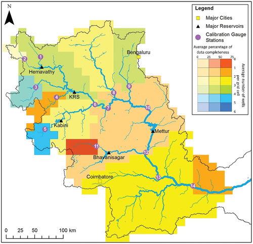
The Cauvery River basin is a large basin (~81 000 km²) in Peninsular India (Fig. 1). The majority of the basin falls within two states, Karnataka (upstream) and Tamil Nadu (downstream), and there has long been tension between the two states over the sharing of water resources within the basin (Sharma et al. 2020).

Figure 1. Map of the Cauvery River basin with key features labelled and location inset. Gauging stations are numbered for clarity; corresponding names can be found in Appendix B (Table B1).

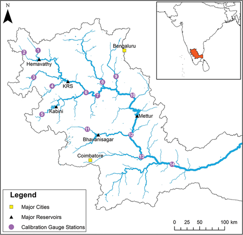
The Cauvery River starts in the Western Ghats mountain range, which extends along the western part of the basin. From here, the river flows across the Mysore plateau and out to the Bay of Bengal through an extensive delta system. There is a significant precipitation gradient across the basin, with average rainfall of more than 3000 mm a⁻¹ in the west, decreasing to ~500 mm a⁻¹ in the east (Ministry of Water Resources 2014). The majority of the rain falls between the months of June and September, during the southwest monsoon. High temperatures result in high levels of potential evapotranspiration, and the latter also varies spatially: from less than 1300 mm a⁻¹ in the west to over 1700 mm a⁻¹ in the east (Ministry of Water Resources 2014).

The topography and geology of the basin are variable (Palamakumbura et al. 2020). The upper catchment is primarily on the Mysore plateau, a high undulating plateau comprising gneiss and various supracrustal rocks. There are also sections of granite in the east, and a mix of gneiss, granite, and charnockite in the deeply weathered domain of the Western Ghats. The midpoint of the catchment is bisected by a band of charnockite with variable topography (250–1400 m). The lower catchment gradually descends with gentle undulations, and is a mix of gneiss, granite, and charnockite, with sedimentary rocks at the delta. The aquifer can be divided into the weathered zone, which consists of saprolite and/or saprock, the fissured zone and unfissured bedrock. Across much of the basin the saprolite layer is missing or very thin (Krabbendam and Palamakumbura 2018). Groundwater flow in bedrock is generally confined to the fissured zone, where fractures can significantly enhance the effective permeability and storage. Fissures generally decrease with depth and yields are reduced significantly into the unfissured bedrock (Dewandel et al. 2006).

The basin is predominantly rural, with several significant urban centres (Bengaluru, Coimbatore, and Mysuru), and approximately 34% of the basin area is irrigated cropland The main crops are rice, sorghum, and maize, and flood irrigation is the most common method used (India-WRIS 2012). Irrigation demand is met from the rivers, through a network of canals (often referred to as command areas), and by groundwater abstractions. Approximately half of the irrigation demand in the basin is met from groundwater (Government of India 2011a), though it is difficult to accurately estimate this due to low levels of regulation and significant private investment in groundwater abstraction infrastructure. Farm bunds are used to harvest rainwater, and rural tanks and check dams hold back surface water flow, to recharge local groundwater (Horan et al. 2021c).

Bengaluru (also known as Bangalore), a city of 8.4 million people (2011), is located on the northeastern boundary of the Cauvery River basin (Government of India 2011b). A large portion of Bengaluru’s water demand is met by water transferred from the Cauvery River, but there is also a dependence on groundwater pumping (Sekhar et al. 2017). In the lower catchment lies the city of Coimbatore, with a population of 1.1 million (2011) (Government of India 2011b). There are high levels of artificial groundwater recharge from leaky pipes and wastewater in the city centres (Sekhar et al. 2017). Urban tanks (or lakes) are employed as a rainwater store, a source of drinking water, and a method of recharging the local aquifer.

The Cauvery basin is heavily regulated. There are several major water transfers around the basin, transporting water within the basin to meet demand from urban and industrial areas. There are also transfers out of the basin which supply water to Chennai, the capital city of Tamil Nadu with a population of 8.7 million (2011). There are multiple large reservoirs in the catchment, with the purpose of providing water supply for irrigation, or dual-purpose irrigation and hydropower. The Mettur dam is the largest dam in the basin, with a reservoir capacity of ~2650 million m³ (Da 2013), and has a significant impact on downstream flows.

Groundwater is an important water resource in the Cauvery basin, and widely abstracted, therefore the tracking of groundwater depth, and a better representation of groundwater processes, is necessary to model the water resources. There are several benefits to considering groundwater depth over a conceptual store: it enables model validation using groundwater as well as streamflow, it allows for an assessment of relevant risks such as groundwater flooding and subsidence, and it can inform water resource management (e.g. required well depths and pump capacities, potential energy and carbon costs for groundwater pumping).

3 Methods and materials

3.1 Model structures

3.1.1 GWAVA

GWAVA is a gridded, semi-distributed, conceptual water resources model (Meigh et al. 1999, Dumont et al. 2012). The model accounts for natural hydrological processes, but also anthropogenic influences (see UK Centre for Ecology and Hydrology (2020) for a detailed description). The spatial and temporal resolution of GWAVA is flexible, with a typical spatial range of 0.1–0.5°, and daily or monthly time steps. It calculates direct runoff and soil moisture for each grid cell using the Probability Distributed Model (PDM) (Moore 2007).

For a given grid cell, the natural processes are calculated for each time step over the whole run period. Water demand (including water for transfers) is then abstracted from the time series of streamflow and groundwater store, and any unconsumed or transferred water is added to the relevant store. Streamflow for the grid cell is then routed downstream (through lakes, wetlands or reservoirs if present), and the processes are repeated for the next grid cell in the stream order. GWAVA outputs typically consist of streamflow time series and various statistics relating to water resources, although any time series of modelled variables can be output.

The groundwater component consists of a conceptual subsurface store for each grid cell, which receives groundwater recharge from the soil moisture storage. Recharge from other sources (e.g. lakes, artificial recharge structures, river channels) is neglected.

Some portion of the groundwater storage, GW_store (mm), is routed as baseflow, BF (mm), according to the following equation:

(1) $BF=G_{route}\cdot {\left(G_{store}\cdot 0.01\right)}^{B{F}_{power}},$(1)

where G_route (routing parameter) and BF_power (recession parameter) are calibratable, and BF has a maximum value of GW_store. Baseflow is added to the surface water store in each grid cell at each time step, prior to river routing.

There is an option for water to drain from the groundwater store (as a simplistic representation of deeper groundwater processes), and any water that drains from the groundwater store is lost from the system. Water abstractions in GWAVA are decoupled, i.e. groundwater demands are not abstracted from the groundwater store at each time step. The GWAVA model does not produce any groundwater time series.

There are a few key limitations to this approach. Firstly, with decoupled groundwater abstraction, the important feedbacks on streamflow from groundwater abstraction and return flow are not captured (de Graaf et al. 2014). Secondly, with no calculated depth to groundwater it is not possible to fully validate the groundwater processes using observed data, i.e. if the conceptual groundwater store was made a model output then changes in groundwater level could be calculated using an approximate, depth independent specific yield, but no absolute values are simulated for comparison with observed data. Finally, in GWAVA the groundwater recharge from water bodies (e.g. lakes, reservoirs, wetlands) is neglected, which can lead to an underestimation in groundwater recharge. These limitations have all been addressed in the model changes described in the following subsection.

3.1.2 GWAVA-GW

In GWAVA-GW, a new groundwater module incorporating additional groundwater processes is added to GWAVA (including small-scale interventions (Horan et al. 2021c)). This includes a full coupling between natural and artificial groundwater processes, such that the change in depth to groundwater due to anthropogenic fluxes impacts the volume of water routed as baseflow, thus addressing a significant limitation in the GWAVA model when applied to regions with significant groundwater.

In this new version of the model, the aquifer is conceptualized as a one-dimensional store in which specific yield can vary with depth. This is represented as a series of simple layers, each of which is assigned a specific yield value. The number of layers and their thickness, which can both vary between cells, are defined by the user based on knowledge of the hydrogeology of the system. Simulation of lateral groundwater flow between cells is not implemented. However, this is considered acceptable since GWAVA is designed for large-scale implementation, typically 0.1–0.5°, and dynamic interaction between the water table and the unsaturated zone is not modelled (Krakauer et al. 2014, Scheidegger et al. 2021). Furthermore, as indicated by a recent detailed hydrogeological and groundwater modelling study (Collins et al. 2020) of a sub-catchment of the Cauvery River basin (Fig. 1), lateral groundwater flow is likely to be a small part of the groundwater balance in such crystalline-bedrock systems.

The groundwater store is recharged from the soil moisture (in a similar manner to GWAVA), but also from lakes and reservoirs, leaky pipes, and artificial recharge structures (tanks, check dams and farm bunds), thereby addressing a second limitation in the GWAVA model. Recharge from large water bodies, such as major reservoirs, is assumed to be at a user-defined constant rate specific to each water body. Recharge from leaky pipes is calculated as a percentage of water abstracted. This is to capture the conveyance loss of water between the point of abstraction and the user, which can be a major source of recharge in urban areas (Sekhar et al. 2017). The percentage conveyance loss is user defined and varies between urban and rural water demands to reflect the different infrastructures.

Small-scale artificial recharge structures included in GWAVA-GW are: urban and rural tanks, check dams, and farm bunds. Each type of structure is lumped for each grid cell, and recharges the groundwater store at a constant rate until empty (they also lose water via evaporation). Farm bunds are low ramps built along the boundaries of fields. Therefore, within the model, they are assumed to be filled by rainfall and surface water runoff, and to recharge at a rate that is dependent on the local soil type. Water held back by farm bunds is assumed to completely infiltrate or evaporate by the end of the day. Check dams are built across small streams, and thus fill from direct rainfall, surface water runoff, and streamflow. Urban and rural tanks are artificial water bodies that also fill via direct rainfall, surface water runoff, and streamflow. Catchment-wide recharge rates are user-defined for check dams, urban and rural tanks. The values chosen should account for soil and aquifer type, as well as the frequency of dredging.

The groundwater store, GW_store (mm), is routed as baseflow, BF (mm), according to:

(2) $BF=\left\{\begin{array}{cc}\lambda \cdot \left(G_{store}-G_{BF}\right),& G_{store}>G_{BF}\\ 0,& G_{store}\le G_{BF}\end{array}\right.,$(2)

where λ is a routing coefficient and GW_BF (mm) is the level of groundwater storage below which there is no baseflow. Baseflow is added to the surface water store in each grid cell at each time step, prior to anthropogenic abstractions and return flows, which is then followed by river routing. GW_BF is generally converted from a store to a depth value h_BF (m) by dividing by the specific yield (accounting for different specific yield values in different aquifer layers, and for unit conversion). This conversion aids comprehension by standardising the units for groundwater-related model inputs and outputs. Depth to groundwater has been included as a model output, allowing for comparison with observed data; this capability is lacking from the GWAVA model.

The parameters λ and h_BF can be calibrated for each grid cell (λ can range from 0 to 0.05, h_BF from 0 to the maximum aquifer depth). Note that these parameters replace the calibratable groundwater parameters from the original model, G_route and BF_power, but are not equivalent (although the routing parameters G_route and λ perform similar functions). Water can be directly abstracted from the groundwater store down to a user-defined maximum depth. The layered aquifer and related routing were tested under artificial recharge, to provide confidence in the application of GWAVA-GW to the Cauvery basin (see Appendix A).

For both GWAVA and GWAVA-GW, initial stores are set during a model spin-up period, with a recommended length of >30 years. Preliminary investigations in the Cauvery basin suggest that depth to groundwater reaches the long-term average depth within 2–5 years of the model start.

3.2 Data sources

The data used to run GWAVA and GWAVA-GW in the Cauvery basin are summarized in Appendix B, Table B2. They were run at a daily time step on a 0.125° × 0.125° grid. The model domain excludes the downstream delta region in Tamil Nadu, which cannot be accurately represented in the GWAVA models as they do not account for tidal processes.

Anthropogenic demands for each grid cell, consisting of domestic, livestock, industrial and irrigation demand, were estimated as follows. Domestic demand was calculated by multiplying population by the legal national water supply requirement: 135 L per capita per day for urban area, and 70 L per capita per day for rural areas (Government of India 2011a). Livestock demand was estimated by multiplying populations of cattle by 77 L per capita per day, and goats and sheep by 5.25 L per capita per day (FAO 2018). Industrial demand was estimated based on the size and type of industry present in each industrial area (KIADB 2020, TIDCO 2020), and scaled using the national estimates reported in the Food and Agriculture Organization (FAO) AQUASTAT database (FAO 2016).

Irrigation demand was determined using a crop factor method, and modelled as 44% efficient based on expert knowledge of irrigation practices in the basin and small catchment studies (this value is within the range of reported efficiencies in India; see Mishra and Dhar 2018, Jain et al. 2019). Of all the water abstracted for irrigation, 30% is returned to surface water as runoff and the rest is assumed to be lost from the system as unproductive evapotranspiration. This is a simplification, since in reality some will be beneficially consumed by the crop (here assumed to be 44% of total water withdrawn), some will be lost to unproductive evapotranspiration (e.g. during conveyance or field application), some will be surface runoff, and some will recharge the groundwater. In the GWAVA and GWAVA-GW models, the lack of groundwater recharge from irrigation will lead to an underestimation of groundwater recharge, and should be addressed in future model developments since this is potentially significant (Ebrahimi et al. 2016). However, it can be challenging to accurately represent irrigation return flow in a large-scale conceptual model, as demonstrated by the range of methods employed by other water resource models (e.g. in CWatM 50% of return flow from irrigation is lost to evaporation and 50% is returned to the channel network (Burek et al. 2020), whereas in the VIC model unconsumed irrigation water is returned to the soil column (Droppers et al. 2020)).

The proportion of water demand sourced from groundwater and the river store varies across the basin, according to data publicly available from the government of India (Government of India 2011a). If water demand cannot be satisfied from the preferred source (if the store is exhausted), then the model allows water to be withdrawn from any available source in the cell to meet demand. If both surface and groundwater stores are depleted, then the demand remains unmet.

The percentage of water lost during conveyance was taken to be 23% for urban systems (urban domestic and industrial demand), and 25% for rural systems (rural domestic and livestock demand) (Government of India 2011a). Water demand is increased by the relevant percentage to calculate the volume of water that must be withdrawn to meet demand. This water is assumed to be lost through leaky pipes and similar infrastructure, so it is added to the groundwater store. Water abstracted for demands but not consumed (sewage, industrial effluents, irrigation runoff, etc.) is added to the river store at a rate of 62% for urban domestic and industrial demand, 0% for rural domestic and livestock demand, and 30% for irrigation demand (Government of India 2011a).

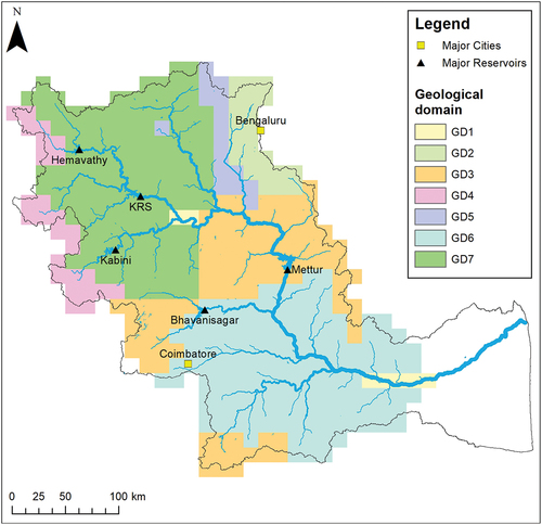
The aquifer parameters (specific yield and depth for each layer) were estimated using a three-layer conceptual model, detailed in Fig. 2, based on a field-validated geology presented in Fig. 3. The geological domains were determined from reconnaissance field visits in the upper Cauvery and analysis of satellite imagery for the whole Cauvery basin (Krabbendam and Palamakumbura 2018); their characteristics are presented in Appendix C, Table C1. In the upper Cauvery six geological domains were identified, and a seventh geological domain was defined in the lower Cauvery. Using Central Ground Water Board (CGWB) district reports and other sources (e.g. Maréchal and Holman 2004, Dewandel et al. 2006, 2010, 2011, Singhal and Gupta 2010, Benoit et al. 2017) each domain was populated with layer thicknesses and each layer was assigned a specific yield value. In general each domain consists of four main layers; these were saprolite, saprock, fissured rock and bedrock. The saprolite and saprock were commonly combined into a single layer in the model as they have similar hydrogeological properties. In the case of the charnokite domain only a thin layer of saprolite was present above the bedrock, meaning this domain was conceptualized as having only two main layers. In the lower catchment and in the lower reaches of the river on the Mysore plateau there are thick layers of alluvium overlying the saprolite/saprock layers, which are underlaid, as elsewhere, by fissured rock and bedrock, meaning this domain has four layers in the model. A groundwater abstraction limit was set for each domain by averaging the observed groundwater depths spatially over the domain and selecting the maximum spatially-averaged depth over the model time period.

Figure 2. Specific yield values at each layer for the different geological domains. Orange lines denote groundwater abstraction limit.

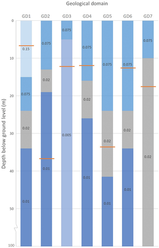
Figure 3. Hydrogeological domains defined for the conceptual groundwater model in GWAVA-GW. For details see Fig. 2.

3.3 Approach to calibration and validation

Both model versions were calibrated and validated using streamflow data from 14 different gauging stations across the basin (Fig. 1). For convenience, these gauges have been numbered 1–14 in this study and the sub-catchments upstream of each gauge are referred to by the corresponding gauge number. These were selected from a set of 28 gauges across the basin, based on completeness of the data, time period covered by the data, and size of the sub-catchment. The data were deemed sufficiently complete if more than half of the data points were labelled as “observed,” not “calculated,” and had at least five consecutive years available, within the years of interest (1980–2014). This threshold may seem low, but raising the limit for the proportion of observed to calculated data left very few gauges to choose from. Additionally, sub-catchments of three or fewer grid cells were excluded, since, for these sub-catchments, there were significant differences between the actual sub-catchment area and the area assumed in the model (due to grid resolution). A description of selected gauging stations and associated sub-catchments, including the years used for calibration and the years used for validation (selected based on consecutive data availability), is presented in Appendix B, Table B1.

Observed depth to groundwater data were used in the calibration and validation of GWAVA-GW. Basin-wide depth to groundwater data were only available from 2007, so data from the period 2007–2014 were considered. Figure B1 in Appendix B shows the density of wells in each sub-catchment, and the average percentage of data points for each well between 2007 and 2014, and depicts the spread and completeness of the available depth to groundwater data. The groundwater wells were grouped by geological domain or by sub-catchment when used for calibration and validation. Note that when groundwater data are averaged spatially over the sub-catchment, this includes the area upstream of each gauge but excludes the area covered by any nested sub-catchments.

GWAVA was calibrated against streamflow data using the GWAVA auto-calibration routine. This routine uses four parameters for calibration: surface and groundwater routing parameters (S_rout, G_rout), a PDM parameter that describes spatial variation in soil moisture capacity (b), and a multiplier to adjust rooting depths (fact). Note that these parameters only affect the natural components of the system. A downhill simplex method (Nelder and Mead 1965) varies these parameters (within an allowed range) to minimize a user-selected objective function, based on absolute difference, Nash-Sutcliffe efficiency (NSE), log NSE, or a non-parametric variant of Kling-Gupta efficiency (KGE). In this study, each objective function was used, and a calibrated parameter set was selected based on a visual inspection of the observed data and modelled streamflow over the calibration period for each sub-catchment. For most sub-catchments, calibrating to the non-parametric variant of KGE gave the best visual fit to the observed streamflow over all aspects of the hydrograph (low flows, peaks, recession limb, etc.).

The parameter BF_power is not included in the auto-calibration routine since calibrating with fewer parameters reduces the risk of overfitting. However, in this study BF_power is manually calibrated to standardize the number of calibrated parameters between GWAVA and GWAVA-GW, so that any improvement in model performance can be attributed to model process changes rather than increased calibration. Additional manual calibration was carried out for gauges downstream of reservoirs, by re-running the auto-calibration routine with a range of different reservoir parameters and selecting the best parameter set based on the objective function and a visual inspection of the flow. Although available, reservoir discharge data were not used for calibration due to low confidence in the data.

For GWAVA-GW, some limits were placed on h_BF and pumping depth for water abstraction for each sub-catchment prior to calibration. The maximum value of h_BF was set to the 75^th percentile of all depth to groundwater data in the sub-catchment, and the maximum pumping depth was set to the maximum observed groundwater depth averaged over each geological domain. This initial coarse “calibration” prevents high levels of demand resulting in improbably deep groundwater values, and accounts for the likely limits on groundwater pumping. In basins where available water generally exceeds water demand, this step may not be required. The model was then calibrated against streamflow using the auto-calibration routine, adapted to vary λ and h_BF in addition to S_rout, b and fact. Reservoir parameters were kept the same as those used in GWAVA, and small-scale interventions were present.

An additional model run was generated to investigate the effect of small-scale interventions on model skill, where GWAVA-GW was calibrated without any small-scale interventions, since there is uncertainty about the impact that these interventions have at the basin scale (Xu et al. 2013).

It should be noted that there is potential for equifinality in the model given the number of spatially variable parameters that can be calibrated. It is necessary for these parameters to be spatially variable, particularly when applying the model over a large and heterogeneous domain, and therefore it is important to reduce the risk of overfitting by calibrating within sub-catchments and geological domains and not for individual grid cells.

When undertaking any form of modelling, it can be challenging to assess model performance when comparing simulated results with observed data. A selection of statistical measures are available, and each has drawbacks. NSE is frequently used in hydrological models, but when used on its own it can be misleading as it emphasizes the fit of high flows over other aspects of the hydrograph (Jain and Sudheer 2008, Gupta et al. 2009). KGE is a multi-objective function which combines comparisons of bias, linear correlation, and variability; it ranges between −∞ and 1. It is an increasingly popular metric in hydrology (Pechlivanidis et al. 2014, Thirel et al. 2015, Knoben et al. 2019), that we have chosen to use here to evaluate model performance. A KGE value of 0.3 is chosen as a threshold to determine whether the model is behavioural or not (midway between the mean flow benchmark and optimal performance values of −0.41 and 1 respectively, as discussed by Knoben et al. (2019). While this threshold is somewhat arbitrary, we are primarily interested in comparative model performance, so this choice is acceptable.

The change in model skill, Δ skill, between GWAVA and GWAVA-GW for streamflow prediction is calculated as:

(3) $\mathrm{\Delta }\mathrm{s}\mathrm{k}\mathrm{i}\mathrm{l}\mathrm{l}=\frac{\left(KG{E}^{GW}-KGE\right)}{\left(KG{E}^{optimal}-KGE\right)},$(3)

where KGE and KGE^GW are the efficiency values for the GWAVA and GWAVA-GW models, respectively, and KGE^optimal is the best possible efficiency value for a given metric (in this case, KGE has an optimal value of 1). A positive value of Δ skill indicates that GWAVA-GW performs better than GWAVA, a zero value suggests similar performance, and a negative value shows that GWAVA-GW performs less well than GWAVA. Since skill change is a relative metric, there are no benchmark values beyond the positive/negative threshold, and the KGE values should always be considered alongside the change in model skill to gain a full understanding. The accuracy of streamflow simulation for each model is compared, but the accuracy of depth to groundwater cannot be compared since only GWAVA-GW outputs depth to groundwater values.

4 Results

4.1 Streamflow

Daily mean streamflow produced by GWAVA and GWAVA-GW is compared to observed daily streamflow at selected sub-catchments across the Cauvery basin, in Table 1 and Figs D2–D4 in Appendix D, with the location and name of the sub-catchment gauges given in Fig. 1 and Appendix B, Table B1. Model performance is assessed over the calibration and validation periods using KGE, by visually comparing the hydrographs, and by evaluating the change in model skill between GWAVA and GWAVA-GW.

Table 1. Kling-Gupta efficiency (KGE) values for calibration and validation runs at each sub-catchment, for Global Water AVailability Assessment (GWAVA) and GWAVA with improved groundwater scheme (GWAVA-GW), and change in model skill (Δ skill) between the two model versions for calibration and validation (Equation 3(3) $\mathrm{\Delta }\mathrm{s}\mathrm{k}\mathrm{i}\mathrm{l}\mathrm{l}=\frac{\left(KG{E}^{GW}-KGE\right)}{\left(KG{E}^{optimal}-KGE\right)},$(3) ).

Sub-catchment	Calibration			Validation
	GWAVA	GWAVA-GW	Δ skill	GWAVA	GWAVA-GW	Δ skill
1. Thimmanahalli	0.37	0.65	0.44	−0.01	0.53	0.54
2. Sakleshpur	0.25	0.32	0.09	0.02	0.09	0.06
3. Kudige	0.15	0.31	0.19	0.45	0.54	0.17
4. K. M. Vadi	−0.12	−0.01	0.10	−0.05	0.06	0.10
5. Munthankera	0.48	0.64	0.31	0.54	0.70	0.35
6. T. Narasipur	0.60	0.72	0.31	0.11	0.33	0.25
7. Kollegal	0.42	0.59	0.30	0.30	0.36	0.08
8. T. K. Halli	0.38	0.53	0.24	0.59	0.71	0.31
9. T. Bekuppe	−1.07	0.33	0.68	−5.23	−1.87	0.54
10. Biligundulu	0.59	0.65	0.15	0.36	0.26	−0.17
11. Thengumarahada	−0.08	0.49	0.53	−0.10	0.04	0.13

Results from gauges downstream of the Mettur dam (i.e. gauges 12 to 14) are not presented here. The streamflow at these gauges is dominated by the operations of the dam; this is clearly visible in Fig. D1 in Appendix D, which shows observed streamflow at gauges upstream and downstream of the dam. The simple reservoir routine present in GWAVA and GWAVA-GW was unable to accurately capture the behaviour of the Mettur dam. Since the results from gauges 12 to 14 do not provide any information on whether the addition of more detailed groundwater representation improves model performance, they are excluded from further analysis.

Table 1 presents the KGE values for the calibration and validation periods for GWAVA and GWAVA-GW, and Δ skill between them, for sub-catchments 1 to 11. Table 1 shows that calibration results for GWAVA-GW are in good agreement with observed streamflow: 91% of sub-catchments have KGE ≥ 0.3. Performance over sub-catchment 4, K. M. Vadi, is low for both GWAVA and GWAVA-GW. Possible causes of poor model performance in this sub-catchment are explored in Section 5.

The validation results are generally lower than for the calibration period: 55% of sub-catchments have KGE ≥ 0.3, and in several sub-catchments (2, 9, 10, and 11) the KGE values for GWAVA-GW drop below the behavioural threshold, despite exceeding it in the calibration period.

GWAVA-GW was also calibrated without small-scale interventions, to determine the impact of these interventions on model skill. By comparing the hydrographs and efficiency metrics of the GWAVA-GW results calibrated with and without interventions, it is clear that the inclusion of small-scale human interventions has a minimal impact on model skill, though it does have a small positive impact on the percentage bias in almost all sub-catchments. The impact of interventions on the average depth to groundwater across the sub-catchments is very small. While it is clear that these interventions have little effect on model skill and model stores at the basin scale in the Cauvery, Horan et al. (2021c) demonstrated their effect on streamflow and estimated evaporation at the sub-catchment scale.

Observed and simulated streamflow are compared over the calibration period for sub-catchments 5, 6 and 10 (Appendix D, Figs D2–D4), along with average rainfall over the sub-catchment. These sub-catchments have been selected to illustrate model performance over a range of hydrological conditions in the basin.

Sub-catchment 5, Munthankera, is a small headwater catchment with low levels of anthropogenic influence and relatively high rainfall levels. Both model versions produce good streamflow simulations in this sub-catchment, though both underestimate the peak flows. GWAVA results have a better match to peak flows compared to GWAVA-GW simulations, but GWAVA-GW has a much better match to the recession limbs (Appendix D, Fig. D2). The skill change for GWAVA-GW in this catchment is Δ skill = 0.35 which, given the low levels of water demand, suggests that the model improvement is not solely a result of implementing the groundwater abstraction coupling that is missing in GWAVA.

Sub-catchment 9, T. Bekuppe, is a larger, drier headwater catchment, with high levels of anthropogenic influence as the city of Bengaluru is situated on its eastern edge. GWAVA tends to underestimate low flows and overestimate peak flows, though some peaks are missed altogether. The performance of GWAVA-GW simulations is varied, providing a good match for the streamflow over 2008, but generally underestimating flows in 2010. Both models overestimate a streamflow peak in late 2010, in response to high rainfall levels in the climatological input data (a total of 147 mm over an 11 day period, with a daily maximum of 59 mm), while the observed flow shows a relatively modest peak of 58 m³ s⁻¹ (Appendix D, Fig. D3).

Sub-catchment 10, Biligundulu, is the largest sub-catchment presented, and shows reasonable agreement between simulated and observed flows (Appendix D, Fig. D4). This is the only sub-catchment where the model skill shows a slight decrease for GWAVA-GW compared to GWAVA results in the validation period, although it is difficult to distinguish model performance based on a visual inspection of the hydrograph. Comparing the individual components of the KGE metric for GWAVA and GWAVA-GW shows that, while the two models have similar levels of linear correlation with observed flow, GWAVA-GW has a larger bias and a higher relative variability compared to GWAVA.

4.2 Groundwater depths and abstractions

Depths to groundwater simulated by GWAVA-GW are compared with observed depth to groundwater data between the years 2007 and 2014 (Figs 4 and 5). There is a tendency for the model simulations to overestimate depth to groundwater across the basin (Fig. 4), particularly in sub-catchments where the groundwater abstractions are also overestimated (Appendix D, Fig. D5). The monthly groundwater depth in sub-catchment 2, Sakleshpur, shows good agreement with the observed data, averaged spatially over the sub-catchment (Fig. 5). Although the simulated long-term average is ~5 m deeper than the observed average, it is within the range of groundwater depths that have been observed in the sub-catchment. The simulated groundwater depth has a tendency to flatten out due to the imposed abstraction depth limit, which is not present in the observed data.

Figure 4. Observed (India-WRIS 2020) and simulated (GWAVA-GW) groundwater levels averaged over time (2007–2014) and over the sub-catchment areas (Fig. 1; Appendix B, Table B1).

Figure 5. Observed and simulated (GWAVA-GW) monthly depth to groundwater, averaged spatially over sub-catchment 2 (Sakleshpur), with the range of observed groundwater depths over the sub-catchment.

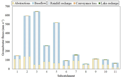
Groundwater fluxes (i.e. vertical flows entering and exiting the groundwater store) were explored to gain insight into the deep groundwater simulated by GWAVA-GW (Fig. 6). Recharge from small-scale interventions is negligibly small over selected sub-catchments (<1 mm a⁻¹), and recharge from lake beds is also small relative to the remaining fluxes. The greatest incoming component across all of the sub-catchments is rainfall recharge, which is particularly high in the sub-catchments in the Western Ghats (sub-catchments 2, 3 and 5) where the rainfall rate is highest. Recharge from conveyance loss (e.g. pipe leakage) is relatively small across all sub-catchments, but is slightly larger in sub-catchment 9, T. Bekuppe, which has a high level of urban water use. Groundwater abstraction is a significant outgoing flux across all the sub-catchments, and in many sub-catchments it exceeds baseflow. Baseflow is added to the surface water store and generally maintains low flows during the dry season. Average baseflow in sub-catchment 9 is very small, and so the simulated low flows are correspondingly small (Appendix D, Fig. D3).

Figure 6. Simulated groundwater fluxes averaged over time (2007–2014) and selected sub-catchment areas. Fluxes are grouped as outgoing (abstractions and baseflow) and incoming fluxes (recharge from rainfall, conveyance loss and from lakebeds). Recharge from small-scale interventions is not included as it is negligibly small. For sub-catchment locations and names see Fig. 1 and Appendix B, Table B1.

The groundwater abstractions are generally overestimated by GWAVA-GW, compared to the abstractions reported by the CGWB (Central Ground Water Board 2009) (Appendix D, Fig. D5). This is particularly true in sub-catchment 2, Sakleshpur, though this may be due to its small size (four grid cells), which tends to exacerbate discrepancies between gridded model output and observed data. In sub-catchment 8, T. K. Halli, GWAVA-GW results underestimate groundwater abstractions, despite a significant portion of the demand in that sub-catchment remaining unmet, because the groundwater abstractions in this sub-catchment are constrained by the maximum pumping depths. Since the average depth to groundwater is in good agreement with observed values, this suggests an underestimation of groundwater recharge.

5 Discussion

5.1 Streamflow

In the Cauvery basin, the streamflow downstream of the Mettur dam is strongly impacted by the dam, and this influence is not well represented by the reservoir simulation routine in the GWAVA and GWAVA-GW models. This presents an opportunity for future research and model development, as an improved reservoir routine has the potential to enhance the model (Horan et al. 2021b), though the accurate representation of reservoir release is a significant challenge, often due to the difficulty obtaining operating rule information (e.g. Zhao et al. 2016, Zajac et al. 2017, Coerver et al. 2018).

In sub-catchment 4, K. M. Vadi, the results from GWAVA-GW are a better fit to the observed streamflow than the GWAVA estimates, but the accuracy is still lower than in other sub-catchments. Interestingly, the VIC model also demonstrates poor model performance in this sub-catchment when calibrated using the same model grid and hydrological data as used in this study (Horan et al. 2021a). This suggests that this particular sub-catchment is not amenable to large-scale modelling; this could result from complex local characteristics that are not well represented in large-scale models, or potentially from poor representation of precipitation in the climate input grid in this area, or other data uncertainties.

In several sub-catchments (2, 9, 10, and 11), the KGE values for GWAVA-GW in the validation period drop below the behavioural threshold, despite exceeding it in the calibration period. Each of these sub-catchments shows a reduction in average observed flow in the validation period compared to the calibration period, with a percentage decrease of 18, 36, 19, and 45%, respectively. Both GWAVA and GWAVA-GW tend to underestimate streamflow during dry periods but provide good estimations of streamflow during wetter periods, which may explain the observed reduction in the KGE metric for these sub-catchments, and highlights the difficulties in calibrating and quantifying model performance using a single metric and over a limited period. This may suggest some missing model components, such as a hands-off flow limit or a mandated minimum reservoir output to maintain environmental flow requirements during dry periods. Alternatively, this trend may be related to the particular periods chosen for calibration and validation, which has been shown to affect model performance (Myers et al. 2021). Ideally, both wet and dry years would be present in both the calibration period and the validation period. However, this was not possible due to limitations in streamflow data availability.

It should be noted that the level of confidence in the observed streamflow is not always high, and a non-negligible portion of the gauge data points are labelled “calculated” rather than “observed” (as discussed in Section 3.3). For instance, in upstream sub-catchments the model simulations regularly show no flow, and this supports many eyewitness accounts of rivers drying out (Srinivasan et al. 2015), but the gauge data do not reflect these observations. It is difficult to quantify these kinds of anecdotal discrepancies.

Overall, the calibration and validation results suggest that the GWAVA-GW model can generally be considered robust and acceptable for streamflow prediction in a heavily human-influenced basin like the Cauvery, though care should be taken in choosing the calibration period. GWAVA-GW shows equal or improved model skill compared to GWAVA in all sub-catchments over the Cauvery basin for the calibration and validation periods, except for a slight reduction of skill in sub-catchment 10, Biligundulu. This demonstrates the importance of a fully coupled groundwater routine in hydrological modelling.

These results are supported by Horan et al. (2021a), where GWAVA-GW (referred to as GWAVA by Horan et al. (2021a)) is shown to have a similar level of predictive skill for streamflow to the VIC and Soil and Water Assessment Tool (SWAT) models in upstream sub-catchments of the Cauvery, and by Horan et al. (2021b), where the performance of various iterations of the GWAVA model is assessed in the Narmada (India) and Cauvery basins, and validated against observed streamflow, reservoir outflow, and groundwater levels.

5.2 Groundwater depths and abstractions

Simulated monthly groundwater depth in sub-catchment 2, Sakleshpur, shows good agreement with the observed data, demonstrating that GWAVA-GW has the capacity to represent the seasonal fluctuations and general trends in depth to groundwater. However, GWAVA-GW tends to overestimate depth to groundwater across the basin, especially in sub-catchments where groundwater abstractions are overestimated.

There is some uncertainty in the observed depth to groundwater data (Bhave et al. 2018, Hora et al. 2019), so it is possible that the observations are underestimating the depth to groundwater in some areas. There are many missing data points in the observed depth to groundwater data (Fig. B1 in Appendix B), and the majority of missing data points have no justification; this is a large source of uncertainty when using this dataset. It is also possible that the water demands in the model are overestimated, leading to an artificial over-abstraction of groundwater (~24% more groundwater abstraction over the basin compared to the values reported by the CGWB (Central Ground Water Board 2009)). In GWAVA-GW, simulated streamflow and groundwater depths in the Cauvery basin are strongly dependent on estimated water demand (see Appendix E), and the methods used to estimate water demand are inherently uncertain. For example, groundwater abstraction for irrigation depends not only on demand but also on the supply of electricity, which is not accounted for in the model. Additionally, the absence of groundwater recharge from irrigation return flow in GWAVA-GW contributes to the overestimation of depth to groundwater to some extent, although there is only a weak correlation (correlation coefficient of 0.2) between irrigation abstraction and root mean square error (RMSE) of depth to groundwater in a sub-catchment.

By considering the simulated groundwater fluxes, abstractions, and depths holistically, it is clear that setting an accurate value for maximum pumping depth can have a large impact on model results, especially in basins that experience water scarcity. This is not a simple task, however, since data are limited, aquifer properties vary non-linearly with depth in basement rocks, and converting point data (such as maximum well depths) to gridded data for model use adds inherent uncertainty. Another option is to implement maximum pumping rates (as in the PCR-GLOBWB (Sutanudjaja et al. 2018) and VIC (Droppers et al. 2020) models), but this also has difficulties. Data on pumping rates are limited, and often require downscaling spatially and temporally, which adds uncertainty. Additionally, this method neglects the dependency of groundwater pumping capacity on groundwater depth (i.e. the reduction in groundwater pumping capacity as depth to groundwater increases).

6 Conclusion

The addition of an improved groundwater scheme to the GWAVA model improves model skill for streamflow prediction across the Cauvery River basin, with a mean increase in skill score of 0.3 in the calibration period and 0.21 in the validation period. The ability to output a time series of estimated depth to groundwater is an important addition to the model, particularly in basins that depend heavily on groundwater, as it allows for integrated water resource management and acts as a useful test for the model (it can reassure the user that the model is getting “the right answers for the right reasons” (Kirchner 2006, p. 1)).

GWAVA-GW provides a balance between a very simple representation of groundwater and a full three-dimensional groundwater representation. It has more complexity than a simple representation, incorporating a layered, spatially variable aquifer, but remains efficient (a standard model run over the Cauvery basin takes 81 seconds for GWAVA and 84 seconds for GWAVA-GW on an Intel computer with 25 GB RAM and a 2.67 GHz CPU, using a Linux operating system). The data requirements to characterize groundwater in GWAVA-GW are low compared to a MODFLOW-style groundwater model, and are adaptable (i.e. the number of aquifer layers are flexible, and other parameters can be estimated or calibrated). The present groundwater scheme could be further improved, by the addition of lateral groundwater movement, by trialling different methods to limit groundwater abstraction, or by addressing the lack of recharge from irrigation.

Small-scale interventions were included but shown to have little impact on model skill, and the recharge to groundwater was negligible at the basin scale.

There were significant challenges in collecting high-quality data for this study which are critical for model performance and assessment, with many streamflow datasets being infilled with calculated values, and missing values in groundwater level datasets. Earth observation data are becoming increasingly abundant at higher resolutions and, if suitably validated with in situ data, could provide an additional data source in future applications of this model.

Overall, the newly developed GWAVA-GW model is a useful tool for integrated water resource assessments in data-sparse regions with high dependence on groundwater, and can be used to better understand interactions between surface and groundwater, and human interventions. This is particularly relevant to future predictions of water resources in regions that are currently over-exploiting groundwater, with potentially harmful future consequences.

Disclosure statement

No potential conflict of interest was reported by the authors.

Additional information

Funding

The research underlying this paper was carried out under the UPSCAPE project of the Newton-Bhabha programme “Sustaining Water Resources for Food, Energy and Ecosystem Services,” funded by the UK Natural Environment Research Council (NERC-UKRI) and the India Ministry of Earth Sciences (MoES), grant numbers NE/N016491/1, NE/N016270/1 and MoES/NERC/IA-SWR/P1/08/2016-PC-II (i), (ii). Authors affiliated with the British Geological Survey (BGS-UKRI) publish with the permission of the Director of BGS. The views and opinions expressed in this paper are those of the authors alone.

Appendices Appendix A:

Testing

To test the functionality of the layered aquifer and baseflow equation described in Section 3.1.2, several simulations have been run with a single grid cell and artificial recharge (Fig. A1). Baseflow and depth to groundwater over time are presented in Fig. A1, and provide evidence that the new model functionality is performing as expected in a small-scale, simplified simulation. Other groundwater interactions, such as abstractions, interventions, and recharge from water bodies, have been ignored. The specific yield parameters match those of the geological domain GD7 (Fig. 2) with h_BF of 18 m, and a range of λ values have been explored. The simulations were run with an initial depth to groundwater of 5 m and no spin-up period.

Figure A1. Baseflow and groundwater depths for a test-case single grid cell under artificial drivers: no recharge, constant recharge (at a rate of 2 mm per time step), and variable recharge (grey line, top right plot). Specific yield values are those of the geological domain GD7 (Fig. 2), and the simulations were run with an initial depth of 5 m, h_BF of 18 m, and λ = 0.001 (solid line), 0.002 (dashed line), 0.005 (dotted line), and 0.01 (dot-dash line).

The results in Fig. A1 demonstrate correct functioning of the new layered aquifer and baseflow equation. Under constant recharge and a low routing coefficient the depth to groundwater decreases until the aquifer “overtops,” with a high routing coefficient depth to groundwater increases until an equilibrium is reached, and in both cases baseflow varies with groundwater store (which is proportional to groundwater depth when specific yield is constant) and ultimately is equal to recharge. For no recharge the depth to groundwater increases, and the rate of increase is higher for a higher routing coefficient. There is a step change in depth to groundwater at 10 m where the value for the specific yield changes (Fig. 2), but no corresponding step change in baseflow since baseflow is a function of groundwater store not depth. For a variable recharge, depth to groundwater demonstrates “seasonal” dependence on recharge and “long-term” trends which, in this case, are determined by the routing coefficient since average recharge is constant. Baseflow fluctuates with recharge and groundwater store.

Appendix B:

Data

Table B1. Description of selected sub-catchments (Fig. 1) including name of gauging station; modelled area; observed average annual rainfall (1988–2014) (Pai et al. 2014) summed over the sub-catchment area; years used for calibration and validation of both models; and percentage of observed data in the streamflow data used for calibration/validation. Note that climate data used only extended to 2014.

Sub-catchment	Modelled area (km^2)	Precipitation over the sub-catchment (mm a^−1)	Calibration		Validation
			Range	Observed data (%)	Range	Observed data (%)
1. Thimmanahalli	1683	1601	2005–2010	32	2010–2014	82
2. Sakleshpur	748	2514	2006–2011	37	2011–2014	68
3. Kudige	2256	2431	1980–1991	72	2012–2014	78
4. K.M. Vadi	2068	1449	1991–2001	49	2001–2012	71
5. Munthankera	1881	2297	1990–2001	50	2001–2012	69
6. T. Narasipur	14 089	1675	1990–2001	43	2001–2009	62
7. Kollegal	21 040	1448	1990–2001	49	2001–2009	60
8. T. K. Halli	8253	785	1988–1997	50	1999–2001	61
9. T. Bekuppe	4883	836	2008–2012	44	2012–2014	78
10. Biligundulu	40 947	1139	1990–2001	78	2001–2012	78
11. Thengumarahada	1511	1487	1990–2001	55	2001–2004	81
12. Urachikottai	53 407	1105	1990–2001	52	2001–2009	82
13. Kodumudi	56 619	1102	1990–2001	58	2005–2011	81
14. Musiri	80 277	1041	1990–2001	55	2006–2011	78

Table B2. Summary of datasets used to build the model.

Input data	Resolution	Source
GWAVA and GWAVA-GW
Precipitation; maximum and minimum temperatures	0.125°, daily	Indian Meteorological Department (Pai et al. 2014)
Elevation	30 × 30 m	NASA Shuttle Radar Mission Global 1 arc second V003 (NASA JPL 2013)
Soil type	30 arcsecond	Harmonized World Soil Database v. 1.2 (Fischer et al. 2008)
Land cover/land use	100 × 100 m, 2005	Decadal land use and land cover across India 2005 (Roy et al. 2016)
Crops	Taluk*, 2005/2006	Central Water Commission & Regional Remote Sensing Centre – West (India-WRIS 2012)
Livestock	5 × 5 km, 2005	CGIR Livestock of the World v. 2 (Robinson et al. 2014)
Population	Village, 2001	Indian Decadal Census (Census of India 2001)
Streamflow gauged data	Country, daily	India – WRIS (India-WRIS 2020)
GWAVA-GW only
Groundwater level data	Country, monthly	Central Ground Water Board, India (India-WRIS 2020)
Interventions	Taluk1* (Karnataka only), 2006–2012	Watershed Development Department, Karnataka (Government of Karnataka 2014)

*An administrative sub-division in India.

Figure B1. Density of groundwater wells for each sub-catchment, and average completeness of the data record for the period 2007-2014.

Appendix C:

Geological characteristics of geo-domains – for hydrogeology of the Cauvery catchment

Table C1. Geological characteristics of geo-domains – for hydrogeology of the Cauvery catchment.

Domain	Domain – full	Topography/relief	Upper aquifer – regolith + fissured zones	Upper aquifer thickness	Lower aquifer – bedrock	Lower aquifer – permeability	Weathering thicknesses (m)	Fissured zone thickness (m)	Transmissivity (m^2/day)^a	Storage (%)^b	Specific yield	Yield (lps)	Source of evidence
GD1	Sedimentary rocks – delta	Low-lying (< 40 m asl) low relief – delta top	Not studied;pProbably dominated by sediment rather than weathered zone	Unknown; likely high	Sedimentary rocks of the Cauvery Delta	Likely to be highly permeable	Cretaceous: 50 Eocene: 80 Orathanadu: 30–70 Miocene main zone: 35 Pliocene: 10–35 Quaternary: 3–25		Min. range: 1–20 Max. range: 550–4500 (Cretaceous: <50 Eocene: 1600–1800 Orathanadu: 10–40 Miocene main zone: <1350 Pliocene: 50–40)		0.1–0.25	Min.: 9 Max.: 63	CGWB district reports Minor irrigation census well failure rates per district Krabbendam and Palamakumbura (2018)
GD2	Bangalore Plateau Dominated by peninsular Gneiss	High undulating plateau; gentle slopes, occasional low inselbergs; more dissected and steeper slopes along edges	Mainly saprock, saprolite only in low-lying areas;upper fissured zone (2–5 m) can be included in this Upper aquifer has sharp and regular boundary with lower bedrock aquifer	~ 5–10 m average; fairly uniform	Poorly fractured; upper layer of sheet joints (common and continuous) best modelled with upper aquifer Background jointing spacing > 5 m Fracture zones, withy spacing 1-5 km	Poor, likely poorly connected background fractures Large fracture zones may give locally high permeability	15–35		Min. range: 0.65–1 Max. range: 125–300	Saprolite: 1–6 Fissured zone: 1–3 Bedrock: 0.1	Saprolite: 0.05–0.1 Fissured zone: 0.01–0.03 Bedrock: 0.01	Min.: 0.1 Max.: 15	CGWB district reports Minor irrigation census well failure rates per district Benoit et al. (2017) working in Anantapur area just northeast of our study area Krabbendam and Palamakumbura (2018)
GD3	Charnockite domain Various granulite facies gneisses – without hydrous minerals	Strongly dissected, high-relief landscape (250–1400 m)	Mainly saprock and thin colluvium	Thin: <5 m	Poorly fractured; lack of sheeting joints Background jointing spacing > 1 m, but very tight Fracture zones, with spacing 1–5 km	Poor to very poor	19–35		Min. range: 0.65–20 Max. range: 250–300	0.015–2	Saprolite: 0.05–0.1 Bedrock: 0.005	Min.: 1 Max.: 2	CGWB district reports Minor irrigation census well failure rates per district Krabbendam and Palamakumbura (2018)
GD4	Deeply weathered domain Peninsular gneiss, granite, charnockite	High plateau (@ c. 900 m), very gentle “double-convex” relief; rivers have very low profiles	Thick and continuous saprolite layer > 5 m thick (clayey sand to sandy clay) Presumably underlain by an equally thick saprock layer	20–?30 m	Not studied; likely variable	Not studied; likely variable			Min. range: 0.65–1 Max. range: 1–125		Saprolite: 0.05 – 0.1 Fissured zone: 0.01–0.03 Bedrock: 0.01	Min.: 1 Max.: 15	CGWB district reports Minor irrigation census well failure rates per district Krabbendam and Palamakumbura (2018)
GD5	Granite domain Granite/granodiorite	Gently undulating with higher (100–400 m) inselbergs; often bare summits	Absent on bare tops; likely to be thicker (saprock and collucium in vales)	From 0 on bar tops to perhaps 15 m in vales	Poorly fractured; remarkable lack of sheeting joints. Background jointing spacing > 5 m Fracture zones, with spacing 1–5 km	Poor, likely poorly connected background fractures; large fracture zones may give locally high permeability	Oct-15	45	Min. range: 5–8.5 Max. range:300–550	Saprolite: 1–5 Fissured zone: 0.5–1.5 Bedrock: 0.3	Saprolite: 0.05–0.1 Fissured zone: 0.01–0.03 Bedrock: 0.01	Min.: 0.1 Max.: 9	CGWB district reports Minor irrigation census well failure rates per district Dewandel et al. (2010) Dewandel et al. (2006) Benoît et al. (2017) All the above are from work conducted in a granite domain in Kudaliar near Hyderabad, north of the study site Krabbendam and Palamakumbura (2018)
GD6	Lower catchment – hard-bedded Peninsular gneiss, granite, charnockite	Gently undulating, gradually descending (300 to 40 m) to delta; locally isolated inselbergs	Not studied; weathering front and thus regolith thickness highly variable Also alluvium widely present?	Not studied; likely highly variable	Variable, as contains peninsular gneiss, granite and charnockite	Not studied; variably poor?	20−35		Min. range: 0.65–8 Max. range: 125–550	0.015–1.5	Saprolite: 0.05–0.1 Fissured zone: 0.01–0.03 Bedrock: 0.01	Min.: 0.1 Max.: 27	CGWB district reports Minor irrigation census well failure rates per district Krabbendam and Palamakumbura (2018)
GD7	Mysore Plateau Peninsular gneiss and various supracrustal rocks	High undulating plateau (600–900 m) gentle slopes, no inselbergs Cauvery falls functions as high-level (c. 600 m) base level	Mainly saprock, saprolite only in low-lying areas; upper aquifer has gradual and irregular boundary with lower bedrock aquifer	~ 5–15 m average; highly variable	Variably fractured; locally densely fractured; mainly with vertical fractures	Fairly good in fractured areas; gradually decreasing with depth as fractures close	1–20		Min. range: 0.65 – 8 Max. range: 125–300 (Mysore district: Min. range: 8–20 Max. range: 500–1500)	Saprolite: 1–6 Fissured zone: 1–3 Bedrock: 0.1	Saprolite: 0.05–0.1 Fissured zone: 0.01–0.03 Bedrock: 0.01	Min.: 0.1 Max.: 18	CGWB district reports Minor irrigation census well failure rates per district Benoit et al. (2017) working in Anantapur area just northeast of our study area Krabbendam and Palamakumbura (2018)

^aRanges are based on the maximum (max.) and minimum (min.) values for each district within the geological domains based on data in CGWB district reports.

^bEffective porosity.

Appendix D:

Additional model results

Figure D1. Daily hydrograph for gauged streamflow at sub-catchment 10, Biligundulu, which is upstream of the Mettur dam, and 12, Urachikottai, which is downstream of the Mettur dam (Fig. 1; Appendix B, Table B1) (India-WRIS 2020).

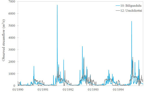
Figure D2. Daily hydrograph for sub-catchment 5, Munthankera (Fig. 1; Appendix B, Table B1), showing observed stream flow (India-WRIS 2020), and simulated streamflow from GWAVA and GWAVA-GW.

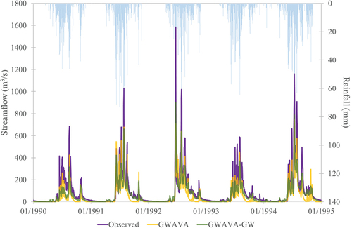
Figure D3. Daily hydrograph for sub-catchment 9, T. Bekuppe (Fig. 1; Appendix B, Table B1), showing observed stream flow (India-WRIS 2020), and simulated streamflow from GWAVA and GWAVA-GW.

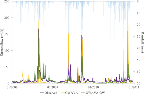
Figure D4. Daily hydrograph for sub-catchment 10, Biligundulu (Fig. 1; Appendix B, Table B1), showing observed stream flow (India-WRIS 2020), and simulated streamflow from GWAVA and GWAVA-GW.

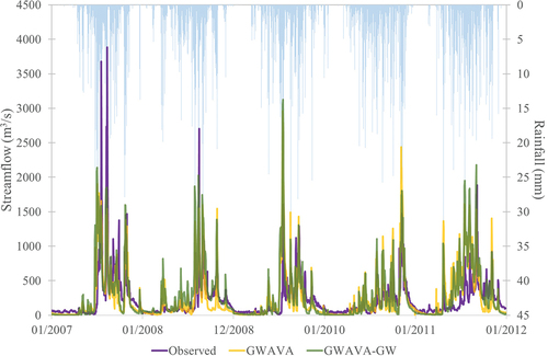
Figure D5. Observed (Central Ground Water Board 2009) and simulated (GWAVA-GW) groundwater abstractions over the sub-catchments (Fig. 1; Appendix B, Table B1).

Appendix E:

Sensitivity

Some model variables were varied to explore the responsiveness of streamflow and groundwater levels to these inputs: the calibrated groundwater parameters λ and h_BF are considered, as are anthropogenic demand and aquifer specific yield (Sy) values. These variables (hereafter referred to as the sensitivity variables) were selected either because they were new to the model (i.e. λ, h_BF and Sy) or because they have a high level of uncertainty (i.e. demands). GWAVA-GW was run for the period 2007–2014 with baseline values (i.e. the inputs and parameters used for calibration), and with each sensitivity variable halved and doubled (unless the variable limit is reached, in which case the maximum or minimum value was used) and all other inputs kept constant, giving a total of eight sensitivity runs. For each run, average depth to groundwater and average streamflow were calculated for each sub-catchment. These metrics are compared to the baseline results for each sensitivity run, and presented as a percentage of the baseline in Fig. E1 (e.g. 100 indicates no change from the baseline; 200 means the value is doubled). When interpreting these results, it is important to remember that groundwater depths are measured as metres below ground level, so an increase in groundwater depth is a decrease in available groundwater.

These results demonstrate that varying the demands has a modest impact on the depth to groundwater and a significant impact on the streamflow across the catchments, and that increasing demand decreases the streamflow and increases the depth to groundwater (and vice versa). Varying demand has a different impact on depth to groundwater and streamflow for the different sub-catchments depending on whether the demand is drawn mainly from the groundwater or surface water stores (e.g. in sub-catchment 11 demand is drawn primarily from the groundwater store, and in sub-catchment 8 demand is drawn primarily from the streamflow).

Varying h_BF has a moderate impact on streamflow across all the sub-catchments. Decreasing h_BF reduces baseflow, since the depth to groundwater will frequently be deeper than h_BF due to groundwater abstractions. However, increasing h_BF has little impact on streamflow. This can be explained by recalling that the volume of water routed as baseflow from the groundwater store is proportional to the difference between the depth to groundwater and h_BF (Equation 2(2) $BF=\left\{\begin{array}{cc}\lambda \cdot \left(G_{store}-G_{BF}\right),& G_{store}>G_{BF}\\ 0,& G_{store}\le G_{BF}\end{array}\right.,$(2) ), therefore if h_BF changes and the depth to groundwater changes by a similar degree, then the volume of baseflow will not change much. Depth to groundwater shows strong sensitivity to h_BF, with increased h_BF leading to large increases in depth to groundwater in sub-catchments 3, 5, and 11. These sub-catchments have the greatest proportion of annual baseflow to abstractions in the baseline run (Fig. 6). For sub-catchment 5, the relationship is nearly linear, as doubling h_BF approximately doubles the depth to groundwater, and halving h_BF approximately halves the depth to groundwater.

Very little responsiveness is shown to variation in specific yield for average streamflow and depth to groundwater, across the sub-catchments. This is because specific yield controls the dynamics of a groundwater system rather than the flow balance, so sensitivity to this parameter would be more evident in the variability rather than the average groundwater depth, i.e. the results would show high sensitivity to specific yield over seasonal time scales but not when averaged over multiple years as in Fig. E1.

The groundwater routing parameter, λ, has some impact on both depth to groundwater and streamflow, though this effect is not consistent across the sub-catchments. Decreasing λ (slower routing) generally results in decreased average depth to groundwater and decreased average flow. These effects are more prominent in sub-catchments with greater levels of baseflow in the baseline run (see Fig. 6).

Figure E1. Average depth to groundwater for the sensitivity runs, and average streamflow for the sensitivity runs, as a percentage of baseline results for each sub-catchment (1–11). The sensitivity variables are: anthropogenic demand, Sy (specific yield), and groundwater parameters λ and h_BF. The dot indicates the result when the sensitivity variable is increased.

References

- Benoit, D., et al., 2017. Geophysical signature location in the South-West of Chad: structural implications. Journal of Geology & Geophysics, 7 (1). doi:10.4172/2381-8719.1000319
- Bhave, A.G., et al., 2018. Water resource planning under future climate and socioeconomic uncertainty in the Cauvery River basin in Karnataka, India. Water Resources Research, 54 (2), 708–728. doi:10.1002/2017WR020970
- Burek, P., et al., 2020. Development of the Community Water Model (CWatM v1.04) – a high-resolution hydrological model for global and regional assessment of integrated water resources management. Geoscientific Model Development, 13 (7), 3267–3298. doi:10.5194/gmd-13-3267-2020
- Census of India, 2001. Provisional population totals. Government of India.
- Central Ground Water Board, 2009. District ground water brochures [online]. Available from: http://cgwb.gov.in/District-GW-Brochures.html [ Accessed 1 February 2021].
- Coerver, H.M., Rutten, M.M., and van de Giesen, N.C., 2018. Deduction of reservoir operating rules for application in global hydrological models. Hydrology and Earth System Sciences, 22 (1), 831–851. doi:10.5194/hess-22-831-2018
- Collins, S., et al., 2020. Groundwater connectivity of asheared gneiss aquifer in the Cauvery River Basin, India. Hydrogeology Journal, 28 (4), 1371–1388. doi:10.1007/s10040-020-02140-y
- Da, T., 2013. Mettur Dam. Water & Energy International, 70 (3), 59–60.
- de Graaf, I.E.M., et al., 2014. Dynamic attribution of global water demand to surface water and groundwater resources: effects of abstractions and return flows on river discharges. Advances in Water Resources, 64, 21–33.
- de Graaf, I.E.M., et al., 2017. A global-scale two-layer transient groundwater model: development and application to groundwater depletion. Advances in Water Resources, 102, 53–67.
- Dewandel, B., et al., 2006. A generalized 3-D geological and hydrogeological conceptual model of granite aquifers controlled by single or multiphase weathering. Journal of Hydrology, 330 (1–2), 260–284. doi:10.1016/j.jhydrol.2006.03.026
- Dewandel, B., et al., 2010. Development of a tool for managing groundwater resources in semi-arid hard rock regions: application to a rural watershed in South India. Hydrological Processes, 24 (19), 2784–2797. doi:10.1002/hyp.7696
- Dewandel, B., et al., 2011. A conceptual hydrodynamic model of a geological discontinuity in hard rock aquifers: example of a quartz reef in granitic terrain in South India. Journal of Hydrology, 405 (3–4), 474–487. doi:10.1016/j.jhydrol.2011.05.050
- Döll, P., et al., 2012. Impact of water withdrawals from groundwater and surface water on continental water storage variations. Journal of Geodynamics, 59-60, 143–156. doi:10.1016/j.jog.2011.05.001
- Droppers, B., et al., 2020. Simulating human impacts on global water resources using VIC-5. Geoscientific Model Development, 13 (10), 5029–5052. doi:10.5194/gmd-13-5029-2020
- Dumont, E., et al., 2012. Modelling indicators of water security, water pollution and aquatic biodiversity in Europe. Hydrological Sciences Journal, 57 (7), 1378–1403. doi:10.1080/02626667.2012.715747
- Ebrahimi, H., Ghazavi, R., and Karimi, H., 2016. Estimation of groundwater recharge from the rainfall and irrigation in an arid environment using inverse modeling approach and RS. Water Resources Management, 30 (6), 1939–1951. doi:10.1007/s11269-016-1261-6
- FAO, 2016. AQUASTAT main database, Food and Agriculture Organization of the United Nations (FAO) [online]. Available from: http://www.fao.org/nr/water/aquastat/data/query/index.html?lang=en [ Accessed 27 January 2020].
- FAO, 2018. Water use of livestock production systems and supply chains – guidelines for assessment (draft for public review). Rome, Italy: Livestock Environmental Assessment and Performance (LEAP) Partnership. FAO.
- Fischer, G., et al., 2008. Global agro-ecological zones assessment for agriculture. Rome, Italy: IIASA, Laxenburg, Austria and FAO.
- Government of India, 2011a. Household & irrigation Census 2011 - Town and Village directory [online]. Available from: https://censusindia.gov.in/DigitalLibrary/MFTableSeries.aspx [ Accessed 2 September 2020].
- Government of India, 2011b. Census” of India 2011: city census. New Delhi, India: Registrar General and Census Commissioner of India, Ministry of Home Affairs.
- Government of Karnataka, 2014. Watershed development department” annual report 2013-2014. Government of Karnataka.
- Gupta, H.V., et al., 2009. Decomposition of the mean squared error and NSE performance criteria: implications for improving hydrological modelling. Journal of Hydrology, 377 (1–2), 80–91. doi:10.1016/j.jhydrol.2009.08.003
- Hanasaki, N., et al., 2018. A global hydrological simulation to specify the sources of water used by humans. Hydrology and Earth System Sciences, 22 (1), 789–817. doi:10.5194/hess-22-789-2018
- Horan, R., et al., 2021a. A comparative assessment of hydrological models in the upper Cauvery catchment. Water, 13 (2), 151. doi:10.3390/w13020151
- Horan, R., et al., 2021b. Extending a large-scale model to better represent water resources without increasing the model’s complexity. Water, 13 (21), 3067. doi:10.3390/w13213067
- Horan, R., et al., 2021c. Modelling small-scale storage interventions in semi-arid India at the basin scale. Sustainability, 13 (11), 6129. doi:10.3390/su13116129
- Hora, T., Srinivasan, V., and Basu, N.B., 2019. The groundwater recovery paradox in south India. Geophysical Research Letters, 46 (16), 9602–9611. doi:10.1029/2019GL083525
- India-WRIS, 2012. River basin atlas of India. Jodhpur: RSC-W, NRSC/ ISRO, Dept. of Space.
- India-WRIS [online], 2020. Available from: https://indiawris.gov.in/wris/#/ [ Accessed 1 September 2020].
- Jain, R., Kishore, P., and Singh, D.K., 2019. Irrigation in India: status, challenges and options. Journal of Soil and Water Conservation, 18 (4), 354. doi:10.5958/2455-7145.2019.00050.X
- Jain, S.K. and Sudheer, K.P., 2008. Fitting of hydrologic models: a close look at the Nash-Sutcliffe index. Journal of Hydrologic engineering/American Society of Civil Engineers, Water Resources Engineering Division, 13 (10), 981–986.
- Jimenez Cisneros, B.E., et al., 2014. Freshwater resources. In: C.B. Field, et al., eds. Climate change 2014: impacts, adaptation and vulnerability. Part A: global and sectoral aspects. Contribution of working group II to the fifth assessment report of the intergovernmental panel on climate change. Cambridge, UK: Cambridge University Press, 229–269.
- KIADB, 2020. Karnataka industrial area development board [online]. Available from: http://en.kiadb.in/ [ Accessed 1 October 2020].
- Kirchner, J.W., 2006. Getting the right answers for the right reasons: linking measurements, analyses, and models to advance the science of hydrology. Water Resources Research, 42 (3). doi:10.1029/2005WR004362
- Knoben, W.J.M., Freer, J.E., and Woods, R.A., 2019. Technical note: inherent benchmark or not? Comparing Nash-Sutcliffe and Kling-Gupta efficiency scores. Hydrology and Earth System Sciences, 23 (10), 4323–4331. doi:10.5194/hess-23-4323-2019
- Krabbendam, M. and Palamakumbura, R., 2018. Gneiss, fractures and saprolite: field geology for hydrogeology of the central Cauvery Catchment, south India. Nottingham, UK: British Geological Survey: NERC Open Research Archive.
- Krakauer, N.Y., Li, H., and Fan, Y., 2014. Groundwater flow across spatial scales: importance for climate modeling. Environmental Research Letters, 9 (3), 034003. doi:10.1088/1748-9326/9/3/034003
- Long, D., et al., 2020. South-to-North water diversion stabilizing Beijing’s groundwater levels. Nature Communications, 11 (1), 3665. doi:10.1038/s41467-020-17428-6
- Maréchal, D. and Holman, I.P., 2004. Comparison of hydrologic simulations using regionalised and catchment-calibrated parameter sets for three catchments in England. UK: Institute of Water and Environment, Cranfield University.
- Meigh, J.R., McKenzie, A.A., and Sene, K.J., 1999. A grid-based approach to water scarcity estimates for eastern and Southern Africa. Water Resources Management, 13 (2), 85–115. doi:10.1023/A:1008025703712
- Ministry of Water Resources, 2014. Cauvery basin. Version 2.0. India: Ministry of Water Resources.
- Mishra, A. and Dhar, D., 2018. India needs to focus on water efficiency [online]. Available from: https://www.livemint.com/Opinion/Cbw6kcycrx0QtCPLKneAHP/India-needs-to-focus-on-water-efficiency.html [ Accessed 7 March 2022].
- Mondal, A., et al., 2016. Hydrologic modelling. Proceedings of the Indian National Science Academy, 82 (3). doi:10.16943/ptinsa/2016/48487
- Moore, R.J., 2007. The PDM rainfall-runoff model. Hydrology and Earth System Sciences, 11 (1), 483–499. doi:10.5194/hess-11-483-2007
- Müller Schmied, H., et al., 2020. The global water resources and use model WaterGAP v2.2d: model description and evaluation.
- Myers, D.T., et al., 2021. Choosing an arbitrary calibration period for hydrologic models: how much does it influence water balance simulations? Hydrological Processes, 35 (2). doi:10.1002/hyp.14045
- NASA JPL, 2013. NASA shuttle radar topography mission global 1arc second. Pasadena, CA, USA: LP DAAC.
- Nelder, J.A. and Mead, R., 1965. A simplex method for function minimization. The Computer Journal, 7 (4), 308–313. doi:10.1093/comjnl/7.4.308
- Pai, D.S., et al., 2014. Developmentof a new high spatial resolution (0.25° X 0.25°) long period (1901-2010) daily gridded rainfall data set over India and its comparison with existing data sets over the region. Quarterly Journal of Meteorology, Hydrology & Geophysics, 65 (1), 1–18.
- Palamakumbura, R., et al., 2020. Data acquisition by digitizing 2-D fracture networks and topographic lineaments in geographic information systems: further development and applications. Solid Earth, 11 (5), 1731–1746. doi:10.5194/se-11-1731-2020
- Pechlivanidis, I.G., et al., 2014. Use of an entropy-based metric in multiobjective calibration to improve model performance. Water Resources Research, 50 (10), 8066–8083. doi:10.1002/2013WR014537
- Pokhrel, Y.N., et al., 2015. Incorporation of groundwater pumping in a global land surface model with the representation of human impacts. Water Resources Research, 51 (1), 78–96. doi:10.1002/2014WR015602
- Reinecke, R., et al., 2019. Challenges in developing a global gradient-based groundwater model (G3M v1.0) for the integration into a global hydrological model. Geoscientific Model Development, 12 (6), 2401–2418. doi:10.5194/gmd-12-2401-2019
- Robinson, T.P., et al., 2014. Mapping the global distribution of livestock. Plos One, 9 (5), e96084. doi:10.1371/journal.pone.0096084
- Roy, P.S., et al., 2016. Decadal land use and land cover classifications across India, 1985, 1995, 2005. ORNL DAAC, Oak Ridge, Tennessee. doi:10.3334/ORNLDAAC/1336
- Safeeq, M. and Fares, A., 2016. Groundwater and surface water interactions in relation to natural and anthropogenic environmental changes. In: A. Fares, ed. Emerging issues in groundwater resources. Cham: Springer International Publishing, 289–326.
- Scheidegger, J.M., et al., 2021. Integration of 2D lateral groundwater flow into the Variable Infiltration Capacity (VIC) model and effects on simulated fluxes for different grid resolutions and aquifer diffusivities. Water, 13 (5), 663. doi:10.3390/w13050663
- Sekhar, M., et al., 2017. Groundwater level dynamics in bengaluru city, India. Sustainability, 10 (2), 26. doi:10.3390/su10010026
- Sharma, A., Hipel, K.W., and Schweizer, V., 2020. Strategic insights into the Cauvery River Dispute in India. Sustainability, 12 (4), 1286. doi:10.3390/su12041286
- Singhal, B.B.S. and Gupta, R.P., 2010. Applied hydrogeology of fractured rocks. 2nd ed. Dordrecht, Netherlands: Springer.
- Srinivasan, V., et al., 2015. Why is the Arkavathy river drying? A multiple-hypothesis approach in a data-scarce region. Hydrology and Earth System Sciences, 19 (4), 1905–1917. doi:10.5194/hess-19-1905-2015
- Subash, Y., et al., 2017. A framework for assessment of climate change impacts on groundwater system formations. In: C.S.P. Ojha, R.Y. Surampalli, and A. Bárdossy, eds. Sustainable water resources management. Reston, VA: American Society of Civil Engineers, 375–397.
- Sutanudjaja, E.H., et al., 2018. PCR-GLOBWB 2: a 5 arcmin global hydrological and water resources model. Geoscientific Model Development, 11 (6), 2429–2453. doi:10.5194/gmd-11-2429-2018
- Thirel, G., et al., 2015. Hydrology under change: an evaluation protocol to investigate how hydrological models deal with changing catchments. Hydrological Sciences Journal, 60 (7–8), 1184–1199. doi:10.1080/02626667.2014.967248
- TIDCO, 2020. TIDCO – Tamil Nadu industrial development corporation ltd [online]. Available from: https://tidco.com/ [ Accessed 1 October 2020].
- UK Centre for Ecology and Hydrology, 2020. GWAVA: global water availability assessment model technical guide and user manual. Wallingford, UK: UKCEH.
- Vanham, D., Weingartner, R., and Rauch, W., 2011. The Cauvery river basin in southern India: major challenges and possible solutions in the 21st century. Water Science and Technology, 64 (1), 122–131. doi:10.2166/wst.2011.554
- Vörösmarty, C.J., Leveque, C., and Revenga, C., 2005. Freshwater ecosystems millennium ecosystem assessment volume 1: conditions and trends. Washington, DC: Island Press.
- Wada, Y., et al., 2013. Human water consumption intensifies hydrological drought worldwide. Environmental Research Letters, 8 (3), 034036. doi:10.1088/1748-9326/8/3/034036
- Winter, T.C., et al., 1998. Ground water and surface water: a single resource. Circular 1139. doi:10.3133/cir1139
- Xu, Y.D., Fu, B.J., and He, C.S., 2013. Assessing the hydrological effect of the check dams in the Loess Plateau, China, by model simulations. Hydrology and Earth System Sciences, 17 (6), 2185–2193. doi:10.5194/hess-17-2185-2013
- Zajac, Z., et al., 2017. The impact of lake and reservoir parameterization on global streamflow simulation. Journal of Hydrology, 548, 552–568. doi:10.1016/j.jhydrol.2017.03.022
- Zhao, G., et al., 2016. Integrating a reservoir regulation scheme into a spatially distributed hydrological model. Advances in Water Resources, 98, 16–31. doi:10.1016/j.advwatres.2016.10.014