A simple method of bias correction for GCM derived streamflow at catchment scale

ABSTRACT

In this study, a simple polynomial bias correction method is developed to correct the bias in the forecasted streamflow (runoff) derived from a global circulation model (GCM). First, a set of polynomial correction factors was derived comparing observed and GCM-derived runoff for a hindcast period (1961–2000) for each of the 11 selected GCMs. The correction factors are used to correct the GCM-derived streamflow for projected periods (2046–2065 and 2081–2100) for the Intergovernmental Panel on Climate Change scenarios A2 and B1 (CMIP3) for the Murray-Hotham catchment of Western Australia. The assumption is that the correction factors derived for each GCM for the observed period (1961–2000) are valid for the projected periods. Results show the method reduces biases considerably for the projected runoff at a catchment scale. The method developed here uses CMIP3 data but it may be applicable to any GCM data, such as CMIP5/CMIP6.

KEYWORDS:

• climate change
• water resources
• bias correction
• streamflow
• GCM

Editor A. Castellarin Associate Editor J. Thompson

1 Introduction

The multiple sources of biases in hydro-meteorological analysis using general circulation models (GCMs) include the selection of GCMs and their ensembles, choice of climate scenarios, downscaling methods and hydrological modelling techniques. Among them, GCMs produce the most bias (Wilby and Harris 2006, Nóbrega et al. 2011) for precipitation (Dibike and Coulibaly 2005) because of incomplete knowledge of geophysical processes at the global scale and scenario uncertainties due to uncertain futures (Ghosh and Mujumdar 2007). This includes the uncertainty involving the teleconnection between climate indices and catchment hydrology (Shams et al. 2018). Hughes et al. (2011) assessed the hydrological response to climate scenarios in the Okavango River catchment in Southern Africa and observed considerable biases in the sign and magnitude of projected flow changes between different climate models. Maraun et al. (2010) reported a lack of reliable information for most hydrological variables derived from GCMs on a scale of less than 200 km. Ehret et al. (2012) noted that such information on hydrological variables from GCMs is too coarse for a realistic representation of most hydrological processes (Blöschl and Sivapalan 1995, Kundzewicz et al. 2007). Therefore, downscaling of hydrological variables to a smaller scale is necessary for hydrological modelling.

Like GCMs, the choice of downscaling techniques may also involve a source of large biases. For example, Dibike and Coulibaly (2005) found an increasing trend of mean annual river flow for downscaled data with the statistical down-scaling model (SDSM) (Wilby et al. 2002) but the trend was opposite with the Long Ashton Research Station Weather Generator (LARS-WG) (Semenov and Barrow 2002). Wood et al. (2004) tested six approaches using a dynamic and statistical downscaling method and found downscaled precipitation varied among the approaches. Recently Hossain et al. (2021a) compared eight interpolation methods (linear, bi-linear, nearest neighbour, distance weighted average, inverse distance weighted average, first-order conservative, second-order conservative and bi-cubic interpolation) to re-grid the CMIP5 decadal precipitation data to the catchment scale.

Selecting an appropriate hydrological model and its parameterization, understanding the underlying assumptions and limitations of the model and estimating the uncertainty are the key elements for assessing the hydrological impact of climate change (New and Hulme 2000, Surfleet et al. 2012). Bae et al. (2011) reported runoff generation during dry seasons might be highly uncertain based on the selection of a hydrological model and potential evapotranspiration (PET) methods. In a study of downscaling regional climate models (RCMs) for the projection of precipitation extremes, Laflamme et al. (2016) illustrated the effect of choice of RCM and GCM driver on downscaling and climate predictions. To address this effect, it is recommended to use multiple GCMs (Wilby et al. 2004, Christensen and Lettenmaier 2007, Bari et al. 2010, Anwar et al. 2011, Islam et al. 2014, Haque et al. 2015, Laflamme et al. 2016, Woznicki et al. 2016, Mehan et al. 2019) which encompass multiple scenarios of possible climate changes in a hydrological regime.

Minimizing biases in hydrological analysis using GCMs involves potential challenges including identifying the actual bias sources as well as quantifying, tracking and intermingling (mixing of uncertainties resulting into new form) of uncertainties at different stages of data analysis. Many bias correction methods have been proposed in the literature, from simple methods using scaling factors (Lenderink et al. 2007, Chen et al. 2011) to complex methods using nonparametric techniques (Ghosh and Mujumdar 2007), probability mapping (Teutschbein and Seibert 2010) and imprecise probability (Ghosh and Mujumdar 2009). A critical review of commonly used bias correction methods for simulating climate change was presented by Maraun (2016), which included the delta change approach, simple mean bias correction and quantile mapping (QM). Teutschbein and Seibert (2010) described bias correction as a re-scaling method to reduce the effects of systematic errors in climate models. Their bias correction refers to the post-processing of RCM output (for temperature and precipitation) at a catchment scale. Piani et al. (2010) provided bias correction of daily precipitation in RCMs over Europe, producing similar statistical distribution with observations. Johnson and Sharma (2011) used six bias correction methods (constant scaling (CS), quantile scaling (QS), QM, monthly bias correction (MBC), simple nested bias correction (SNBC) and nested bias correction (NBC)) to correct uncertainties in GCM rainfall scenarios across Australia. Teutschbein and Seibert (2012) reviewed available bias correction methods and evaluated them through correcting an ensemble of 11 different RCMs’ simulated temperatures, precipitation and monthly mean streamflow and flood peaks. Bias correction methods for daily precipitation considering wet and dry days are proposed by Piani et al. (2010) and Hempel et al. (2013) while methods for a wide range of time scales are proposed by Mehrotra and Sharma (2015, 2016) and Johnson and Sharma (2012) respectively.

Correction approaches include linear scaling, local intensity scaling, power transformation, distribution mapping and the delta-change approach. Ghosh and Mujumdar (2007) developed nonparametric methods for modelling GCM and scenario uncertainties in drought assessment, where samples of a drought indicator were generated with downscaled precipitation from available GCMs and scenarios. In another study, Ghosh and Mujumdar (2009) used an imprecise probability approach where probability is represented as an interval grey number. Recently, Hossain et al. (2021b, 2021c) showed substantial bias (drift) in GCMs’ CMIP5 decadal precipitation and proposed alternative drift correction methods using several skill scores. Among the available bias correction methods, it is hard to choose the most appropriate method because of their varying strengths and weaknesses. The factors influencing the performance of a bias correction method may include the objective of the study (e.g. bias correction of rainfall, temperature, flood peak), time scale considered (e.g. daily, monthly, seasonal, annual), desired level of bias correction, resource availability and assumptions made in the process.

Most of the above bias correction methods use some form of statistical tool, technique, measurement or relationship developed or mapped using observed and simulated data of a particular hydrological parameter (rainfall, temperature, runoff or flow, etc.) for a hindcast or control run period. Next, the tool or relationship developed for the hindcast period is used in correcting the projected simulation. In some cases, bias correction methods correct a parameter (such as daily rainfall) which is subsequently used to simulate the other parameter (such as runoff) (Christensen and Lettenmaier 2007). Applying one bias corrected parameter (such as rainfall) in simulating the other parameter in a hydrological analysis does reduce the biases along the process, which can be considered partial bias correction relative to the bias correction of the end product such as runoff.

Although a considerable number of studies have been conducted for bias correction along the process, a very limited number of studies have focused on the bias correction of GCM-derived runoff (e.g. the end product in hydrological modelling) at a streamgauge level. In a previous study by Islam et al. (2014), a considerable amount of bias was found in GCM-derived runoff for the projected periods of 2046–2065 and 2081–2100 in the Murray-Hotham catchment of southwest Western Australia (SWWA). It was reported that the total biases are the product of individual bias generated from the downscaling technique, hydrological model selection and model parameterization. As a result, the use of GCM-derived runoff remains futile for practical purposes in real-life decision making for water resources management. For this reason, a method of post-processing bias correction becomes necessary for GCM-derived runoff for catchment management. Therefore, the objective of this study is to develop a new post-processing bias correction method for GCM-derived runoff at the catchment scale. The method was calibrated and validated successfully, correcting biases of GCM-derived annual runoff at a gauging station in the Murray-Hotham catchment in SWWA. The method was then applied to correct the future projections of streamflow at the gauging station.

2 Study area, data and methods

2.1 Study area

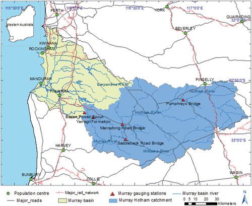
The Murray-Hotham River catchment (6736 km²) of SWWA was selected for this study. The catchment is located approximately 120 km southwest of Perth, the capital of Western Australia. There are three main rivers dominating the catchment: Murray, Williams and Hotham. The Williams and Hotham rivers are the main tributaries of Murray River. The catchment receives around 500 mm of rainfall annually. The catchment is geologically dominated by the Darling Plateau, which progresses from steep valleys in the west to broad undulating valleys in the east. The majority of the east of the catchment is cleared for agricultural purposes. In the west part, it is largely covered by Jarrah (Eucalyptus marginata) and Marri (Corymbia calophylia) forest. The catchment experiences a Mediterranean type of climate with cool, wet winters and hot, dry summers. There are a number of stream gauging stations throughout the Murray-Hotham River catchment, among which five gauging stations (Pumphreys Bridge, Marradong Road Bridge, Saddleback Road Bridge, Yarragil Formation, Baden Powell Water Spout) were studied by Islam et al. (2014) (Fig. 1). Based on the availability of data, Baden Powell station was selected for this study.

Figure 1. Major rivers and gauging stations in the study area: Murray-Hotham catchment of Western Australia.

2.2 Data

GCM data are available from the past three Coupled Model Intercomparison Project experiments: CMIP3 (Phase 3), CMIP5 (Phase 5) and CMIP6 (Phase 6). These correspond to the Intergovernmental Panel on Climate Change (IPCC)’s Fourth, Fifth and Sixth Assessment Reports (AR4, AR5 and AR6) respectively. All CMIP (CMIP3, CMIP5 and CMIP6) datasets contain output from a large number of GCMs. Subsequent CMIPs include more models and use more advanced simulations. Different CMIPs use different scenarios describing the amount of greenhouse gas in the future atmosphere. CMIP3 used scenarios from the IPCC’s Special Report on Emissions Scenarios (SRES) (AR4), CMIP5 uses Representative Concentration Pathways (RCPs) (AR5) and CMIP6 (AR6) considers the impact of socioeconomic conditions (e.g. population, economy) on greenhouse gas emissions by linking RCPs to socioeconomic pathways (SSPs). It should, however, be noted that there is an overall consistency between the projections of different CMIPs for both large-scale climate patterns and the magnitudes of future climate change. Tian and Dong (2020) reported that there is a strong similarity in the pattern of global tropical precipitation among the three generations of CMIP (CMIP3/5/6) models, with a high correlation among them (r² = 0.98 between CMIP3 and CMIP5, r² = 0.98 between CMIP5 and CMIP6, and r² = 0.94 between CMIP3 and CMIP6). This indicates that all three of these generations of CMIP models share important successes and also contain similar systematic errors (Tian and Dong 2020). This provides flexibility in choosing precipitation data from any CMIP future projection in order to develop a bias correction method. In this paper, 11 GCMs (CSIRO-MK3.0, CSIRO-MK3.5, GFDL-CM2.0, GFDL-CM2.1, GISS-ER, CNRM-CM3, IPSL-CM4, MIROC3.2, ECHAM5/MPI-OM, MRI-CGCM2.3.2 and CGCM3.1) were chosen from the CMIP3 (AR4) (IPCC 2007) database to download the precipitation data for two emission scenarios, A2 and B1 (Intergovernmental Panel on Climate Change (IPCC) 2000). The basis for selection of AR4 data is also because the only paper published on Murray-Hotham catchment in Western Australia which used AR4 data reported significant bias (Islam et al. 2014). Bari et al. (2010) found these models suitable for the Australian climate and they were also used by Islam et al. (2014). In the current paper, we develop a simple bias correction method which can be applied in any CMIP experimental output (e.g. CMIP3/5/6). We used AR4 (CMIP3) data in this study in order to compare it with the published results on this catchment using AR4 data (Islam et al. 2014) and check whether this method could improve the bias.

The observed rainfall data (5 km × 5 km grid) and streamflow data at five gauging stations of the study area were collected from the Bureau of Meteorology (BoM), Government of Western Australia. Based on its continuous availability, the data for Baden Powell station was used in this study. However, this method can be applied to any other gauging station having continuous data. The GCM data for the A2 and B1 scenarios were downscaled to a 5 km × 5 km grid using the Bureau of Meteorology Statistical Downscaling Model (BoM-SDM) (Timbal et al. 2009) for the hindcast (1961–2000) and simulated periods (mid-century: 2046–2065 and late century: 2081–2100).

2.3 Hydrological modelling

Hydrological modelling was performed using the Land Use Change Incorporated Catchment (LUCICAT) model (Bari and Smettem 2003). LUCICAT is a distributed conceptual model capable of predicting impacts of climate change and land use change on streamflow and salinity. The selected catchment (large) is broken into small sub-catchments termed response units (RUs) which are the building blocks of the model. The model has three modules: (i) geo-processing module, (ii) rainfall processor, and (iii) main module. The geo-processing module organizes linkage of the RUs, channel network and nodes for a catchment based on the order of flow among the RUs, the channels and nodes of the RUs, and the flow direction in the channels depending on elevation of the nodes (upstream and downstream). The rainfall processor produces daily, monthly and annual rainfall and pan evaporation for each of the RUs based on three rainfall stations for point observations or from four grids for grid rainfall data nearest to the centroid of each of the RUs. The main module consists of three components: (a) water balance model, (b) salt balance model, and (c) stream flow routing.

As building blocks, RUs contain catchment attributes (e.g. soil depth), hydrological attributes (e.g. groundwater level), and land use change or climate change attributes, and each building block consists of dry, wet and subsurface stores: a saturated groundwater store and a transient stream zone store. The main module takes the rainfall and pan evaporation file (generated by the rainfall processor) as input to generate runoff from each of the RUs, which is then routed through the channel network following principles of open-channel hydraulics. The model is capable of producing flow at any nominated node. The calibration of the model is carried out through a trial and error process against a set of calibration criteria at the gauging station of a catchment.

The modelling process can be summarized in two broad steps: (1) calibrating the LUCICAT model and (2) running the model to generate rainfall and runoff for climate scenarios. The calibration process has five basic steps: (a) preparation of input files for the model, which includes (i) preparation of catchment attributes and (ii) preparation of rainfall files for the calibration and validation period; (b) using the rainfall processor of the model, processing the rainfall for the catchment’s RUs; (c) taking the processed rainfall and running the model to process runoff for the RUs; (d) comparing the simulated flow with the observed flow at the gauging station considering a set of calibration criteria; (e) adjusting the catchment attributes, soil attributes, hydrological and other parameters and re-running the model; this step is repeated until the model is calibrated against the set of calibration criteria. The calibration criteria include a joint plot of observed and simulated daily flow series; scatter plot of monthly and annual flow; flow period error index (EI); Nash-Sutcliffe efficiency (NSE); explained variance; correlation coefficient (CC); overall water balance (E); and flow duration curves. The EI indicates the difference between the daily non-zero flow periods of observed and modelled flow. Overall water balance (E) is a measure of the difference between mean daily observed flow and mean daily modelled flow for the period. The catchment attribute files include RU attributes, channel attributes and nodal attributes. The model takes these attributes as ArcGIS shape files. The required model data were obtained from the Bureau of Meteorology, Australia, including other input attribute files such as evapotranspiration, land use, groundwater storage, and soil profile. The model is capable of reading both point rainfall data and grid rainfall data to process rainfall for the RUs. The analysis of results was mainly focused on the catchment spatial average rainfall for RU 135. This RU (135) was selected because it is the last link in the sub-catchment network which represents overall catchment behaviour.

Here, grid rainfall data was used to calibrate the model at the gauging station for 1960–2004 and validated for 2005–2009. The target statistical criteria for calibration for daily streamflow for the gauging station include: (a) NSE and CC values should be greater than 0.5 and 0.75, respectively; (b) daily flow-duration curves should closely match; and (c) the modelled mean annual streamflow for all gauging stations must be within ±5–10% of the observed flow (Bari et al. 2009). The calibration criteria for NSE were also selected according to the scheme given by Henriksen et al. (2008): poor (0.2–0.5), fair (0.5–0.65), very good (0.65–0.85) and excellent (> 0.85).

Annual rainfall and runoff were then projected for the simulated periods (2046–2065 and 2081–2100) for the A2 and B1 scenarios, and the corresponding annual bias was estimated and compared with the observed data. Detailed information on hydrological modelling of the Murray-Hotham River catchment using LUCICAT can be found in Islam et al. (2014).

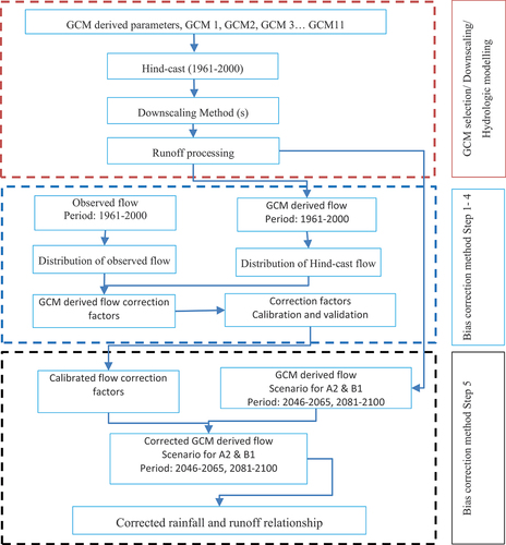
2.4 Development of post-processing bias correction method

A new post-processing bias correction method is developed in this paper which is schematically shown in Fig. 2. The method has three major tasks: part 1 describes the biases inherited in GCM selection, downscaling techniques and hydrological modelling for runoff (streamflow) processing; part 2 shows the development of bias correction factors comparing observed and GCM-derived streamflow through calibration and validation processes; and part 3 indicates the final corrected GCM-derived streamflow and rainfall and their relationship for the future projected time period. The observed runoff data at the stream gauging station was used to calibrate and validate the bias correction method. How the flows obtained from driving the hydrological model with GCM-derived forcing data for a particular GCM compare with the observed flow at a gauging station, in fact, provides the basis for the development of bias correction factors for a particular GCM. Therefore, observed stream flow data is necessary to assess inherent biases of the GCM-derived flow for a particular GCM. It is understood that GCMs are not very good at simulating climate extreme specific to a particular year (as observed in simulating annual flow). Therefore, to capture climate extremes, the (lower) 25th percentile and (upper) 75th percentile of observed and simulated data were used to estimate correction factors. Hence, the availability of a longer period of observed flow data is expected to provide a better comparison between the observed and the GCM-derived flow data to derive the correction factor. A direct comparison approach was adopted to derive the correction factors (as shown in step 2 below). Later the same correction factor is applied to correct biases of the GCM-derived flow for different climate scenarios.

Figure 2. Schematic representation of the bias correction method and corrected flow for GCMs.

Previous studies such as Teutschbein and Seibert (2012) used dry years for calibration and wet years for validation. Such an approach may not capture the GCM’s whole range of climate variabilities (e.g. declining trend in rainfall or runoff or extreme wet or extreme dry). Here, attempts are made to capture these climate variabilities in a different way for calibration and validation. The upper and lower 25th percentile (annual flow of 20 years out of 40 years) data are used for calibration and the remaining (25th–75th) percentile data are used for validation. The key advantage of selecting the upper and lower 25th percentile of data for calibration is to capture the climate variability (including extremes such as wet or dry) and changes as depicted by different GCMs in simulating the observed (annual flow) data. It is assumed that the upper and lower 25th percentile of data contains a higher level of biases representing extremes (wet or dry). The validation method with the 25th–75th percentiles (annual flow) provides greater confidence for bias correction for future projected streamflow. The steps of the bias correction method are given below.

Step 1: Arrange observed and GCM-derived (annual flow) streamflow for the hindcast period (1961–2000) at a gauging station in descending order and take the 1st–25th percentile and 75th–100th percentile data to derive correction factors for individual GCMs. Mathematically, this is expressed as:

(1) $O_i=O_1<O_2\dots \dots \dots \dots \dots \dots \dots \dots O_{39}<O_{40}$(1)

(2) $X_j=X_1<X_2\dots \dots \dots \dots \dots \dots \dots \dots X_{39}<X_{40}$(2)

where $O$ $=Observedannualflow$

$X=GCMderivedannualflow$

$i=1,2,3\dots \dots 9,10and31,32,33\dots \dots \dots 39,40.$

$j=1,2,3\dots \dots 9,10and31,32,33\dots \dots \dots 39,40.$

Step 2: Actual correction factors ($C{F}_a$) for the calibration period (within the hindcast period) for a GCM are developed through matching GCM-derived annual flow (DAF) with the observed annual flow (OAF) of 1st–25th percentile and 75th–100th percentile data as selected and ordered sequentially in step 1.

(3) $C{F}_a=\frac{O_i}{X_j}=\frac{O_1}{X_1},\frac{O_2}{X_2},\dots \dots \dots \dots \dots \dots \dots ..,\frac{O_{39}}{X_{39}},\frac{O_{40}}{X_{40}}$(3)

Step 3: Actual correction factors ($C{F}_a$) for the 20-year calibration period (out of the 40-year hindcast period) are plotted against corresponding simulated DAF and a best-fit polynomial relationship (e.g. second order) derived from the plot. Based on this polynomial relationship and using their polynomial coefficients, the polynomial correction factors $\left(C{F}_p\right)$ can be calculated for a particular value of simulated DAF. It is important to note that a higher order polynomial could lead to over-fitting the relationship. Therefore, identification of the best-fit polynomial is a trial and error process. Steps 1–3 are considered the calibration part of the bias correction method. Mathematically, $C{F}_p$ can be expressed as:

(4) $C{F}_p=aX+b{X}^2+c$(4)

where represents the polynomial correction factor; X is DAF data for the 20-year calibration period (out of the hindcast period) for a GCM as outlined in step 1 and step 2; and a, b and c are polynomial constants.

Step 4: The polynomial relationship between correction factors and simulated DAF data for a GCM developed through calibration (in step 3) is used to derive $C{F}_p$ for correcting DAF data (25th–75th percentile) for the validation period of 20 years (out of the 40 years of the hindcast period). The corrected DAF is calculated by multiplying the simulated DAF with the derived for a particular flow for a GCM. This part is considered validation of the bias correction method. Mathematically, this can be expressed as:

(5) $C{F}_{p,GCMDAF}=aX+b{X}^2+c$(5)

(6) $GCMDA{F}_c=C{F}_{p,GCMDAF}\times X$(6)

where represents the polynomial correction factor for a DAF for a GCM, X is any DAF data for a GCM (either for validation period or future projected periods) for which the correction factor is calculated and $GCMDA{F}_c$ is the corrected DAF of a GCM. Here, the performance of calibration and validation are measured using the goodness of fit of DAFc with OAF and various statistics such as NSE, CC and E.

Step 5: Once validated in step 4, the same process can be used for the future projected periods (2046–2065 and 2081–2100), assuming the polynomial relationship remains the same. This assumption is reasonable because of the use of observed and modelled statistics of the current climate to force the model output for the future period (Johnson and Sharma 2012). This means the bias of hindcast and future simulated data may not show a significant change.

The process described in steps 1 to 5 for bias correction of DAF is for a particular GCM. Therefore, these steps are repeated to correct DAF for each of the GCMs in an ensemble.

3 Results

3.1 Biases in GCM DAF

The biases in GCM DAF were investigated at a gauging station (Baden Powell) and compared with OAF using a time series plot and cumulative time series plot (Fig. 3) for the hindcast period (1961–2000). The GCM DAF values for 11 GCMs are plotted against the corresponding OAF values for the hindcast period at Baden Powell gauging station to compare the skills of GCMs in generating annual flow at a gauging station level (see the Appendix, Fig. A1). The goodness of fit was checked using NSE, CC and E. The results are presented in Table 1. In addition to these time-series-oriented metrics (NSE, CC, E), the spatial correlation of GCMs could be checked using bias-insensitive metrics such as fractional skill score (FSS) and spatial efficiency (SPAEF) (Ahmed et al. 2019, Hossain et al. 2021b). FSS is used to assess the spatial relationship between model-simulated and observed data. FSS varies between 0 and 1, where 0 indicates no relation and 1 refers to a perfect relationship between the observed and simulated data. SPAEF provides one robust spatial relationship metric considering three statistics: Pearson correlation, coefficient of variation, and histogram overlap (Demirel et al. 2018, Ahmed et al. 2019). However, FSS and SPAEF were not considered in this study as the method developed here utilized time series data for a particular location (i.e. a gauging station).

Table 1. Comparative analysis of goodness of fit between GCM DAF and OAF.

	CCM	CNRM	CSIRO	CSIRO2	GFDL1	GFDL2	GISSR	IPSL	MIROC	MPI	MRI
NSE	−1.44	−4.08	−2.19	0.03	−0.39	−0.51	−0.23	−1.44	−3.08	−1.83	−0.48
CC	0.40	0.19	0.30	0.65	0.52	0.52	0.51	0.46	0.44	0.44	0.43
E	0.16	0.72	0.24	0.09	0.35	0.23	0.09	0.46	0.51	0.31	0.29

Figure 3. The state of bias in GCM-derived annual flow for the hindcast period (1961–2000) at Baden Powell gauging station: (a) time series plot, and (b) cumulative time series plot.

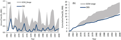
The results show significant dissimilarties between GCM DAF and OAF (Fig. 3 and Table 1). GCM DAF values also show low skills in picking up on particular wet or dry years (Fig. 3(a)). This is because the different GCMs manifest wet or dry years in different ways. Examination of DAF against OAF at the gauging station in Murray-Hotham River catchment for the hindcast period (1961–2000) reveals that GCMs have little skill in simulating annual flow for a particular year. The time series plot (Fig. 3(a)) shows that DAF has a tendency to produce high flow in different years with respect to the OAF. A plot of cumulative DAF and OAF shows that GCM DAF values are relatively larger than OAF values, with wide spectrum (Fig. 3(b)). The NSE values in Table 1 show little similarity among DAF and OAF. For example, NSE values for all GCMs are negative, varying from −0.23 to −4.08 (except CSIRO2 with an NSE of +0.03). The range of NSE varies between 1 and −∞, where 1 indicates a perfect fit and any value lower than zero indicates that the mean value of the observed time series would have been a better predictor than the model (Krause et al. 2005). The CC values also do not show a promising relation (0.19–0.65) for different GCMs.

E is a measure of over- or under-prediction of DAF compared to OAF. The range of E values (0.09–0.72) indicates over-prediction of DAF for all GCMs (Table 2). As GCM DAF shows significant biases with OAF, these GCM-derived values may not be suitable for use in water resources planning (Ehret et al. 2012). Ehret et al. (2012) reported the reasons for biases in model prediction of precipitation, which include (i) the resolution of GCMs (Kundzewicz et al. 2007), (ii) the difficulties with respect to intensity (especially extremes) and intermittancy (Ines and Hansen 2006), and (iii) the challenges in achieving a correct spatial and temporal distribution across regions and seasons (Maraun et al. 2010). This scaling problem may be overcome to some extent through downscaling of GCM data (using a statistical downscaling technique and/or dynamic downscaling through nesting RCMs). Sunyer et al. (2012) documented a comparison of five statistical downscaling methods using results from four RCMs driven by GCMs. There is a need to focus on extreme event generation while downscaling the GCM data, as downscaling methods show significant uncertainty in the downscaled projected changes, especially in the extreme event statistics.

Table 2. Summary of statistics (NSE, CC and E) measuring the calibration and validation performance for all GCMs.

	Calibration			Validation
	NSE	CC	E	NSE	CC	E
CCM	0.42	0.98	0.30	0.98	0.98	−0.05
CCM:C	0.99	1.00	0.00	0.96	0.98	−0.09
CNRM	−0.84	0.98	0.83	−1.06	0.95	0.57
CNRM:C	0.97	0.99	0.00	0.98	0.97	0.00
CSIRO	0.20	0.99	0.39	0.88	0.99	0.03
CSIRO:C	0.98	0.99	0.00	0.92	0.99	0.10
CSIRO2	0.85	0.98	0.18	0.96	0.97	−0.02
CSIRO2:C	0.98	0.99	0.00	0.99	0.98	−0.01
GFDL1	0.79	0.97	0.29	−0.06	0.95	0.43
GFDL1:C	0.97	0.98	0.00	0.93	0.95	0.01
GFDL2	0.74	0.98	0.27	0.77	0.98	0.18
GFDL2:C	0.97	0.99	0.00	0.98	0.98	0.03
GISSR	0.90	0.99	0.13	0.99	0.98	0.02
GISSR:C	0.99	0.99	0.00	0.97	0.98	0.06
IPSL	0.17	0.93	0.50	−0.41	0.97	0.40
IPSL:C	0.95	0.98	0.00	0.99	0.99	−0.03
MIROC	−0.91	0.99	0.74	0.63	0.96	0.17
MIROC:C	0.92	0.96	0.00	0.89	0.98	0.15
MPI	0.05	0.99	0.48	0.83	0.91	0.07
MPI:C	0.96	0.98	0.00	0.95	0.95	0.08
MRI	0.84	0.97	0.22	0.25	0.98	0.38
MRI:C	0.95	0.98	0.00	0.95	0.98	0.07

There is no RCM data available for the catchment (Murray-Hotham) under investigation in this study, but a few studies have sused RCM in other areas of Australia. To produce finer scale regional climate projections for southeast Australia, the NARCliM (N1.0) (New South Wales (NSW)/Australian Capital Territory (ACT) Regional Climate Modelling project) was developed (Evans et al. 2014, Fita et al. 2016). NARCliM (N1.0) provides a comprehensive dynamically downscaled climate dataset for the CORDEX-Australasia region (50-km resolution) and southeast Australia (10 km-resolution). Nishant et al. (2021) presents the expansion of NARCliM N1.0 to NARCliM N1.5, adding the ensemble to 24 members by evaluating the performance of RCM projections for southeast Australia. However, systematic errors remain in the reproduction of hydrologically relevant variables of present-day climate using a GCM-RCM model (Ehret et al. 2012, Muerth et al. 2013, Fita et al. 2016, Nishant et al. 2021) as well as statistical/dynamic downscaling techniques (Wilby et al. 2004, Wood et al. 2004, Randall et al. 2007, Piani et al. 2010, Chen et al. 2011a, Hagemann et al. 2011, Rojas et al. 2011, Haddeland et al. 2012, Johnson and Sharma 2012).

3.2 Calibration and validation of the bias correction method

This section presents the results of calibration (steps 1–3) and validation (step 4) of the bias correction method. The calibration and validation performance are measured using same goodness-of-fit statistics: NSE, CC and E.

The calibration period (20 years) was designed with the top and bottom 25th percentile of annual flow data for the hindcast period (1961–2000) at the Baden Powell gauging station. The remaining 20 years of annual flow data, consisting of the 25th to 75th percentile annual flow, are used for validation of the method. An example of the process of calibration and validation of the bias correction method for the output of one GCM (CNRM) is summarized in Fig. 4. In step 1: First, DAF and OAF data for the hindcast (1961–2000) were organized in descending order to group them into two 20-year periods for calibration and validation. The top and bottom 25th percentile data of DAF and OAF are selected to derive correction factors (CF) through calibration (Fig. 4(a)). A scatter plot of ordered DAF (DAF_o) against ordered OAF (OAF_o) for the calibration period manifested systematic bias in DAF (Fig. 4(a)) for CNRM. In step 2: a set of actual correction factors ($C{F}_a$) is derived through matching the ordered DAF with the ordered OAF (Fig. 4(b)). In step 3: A best-fit polynomial curve of second degree was set to develop a relationship between DAF and CF_a (Fig. 4(b)). Using the polynomial relationship and their polynomial coefficients, the polynomial correction factor (CFp) for any value of DAF for CNRM can be calculated. The level of corrections of CF required fitting into the best-fit polynomial relationship (equation) to obtain CFp.

Figure 4. Calibration and validation of the bias correction method for CNRM at Baden Powell gauging station: (a) DAF and OAF for calibration period with ordered DAFo and OAFo; (b) polynomial relationship between CFa and DAF; (c) transformation of CFp in the relationship; (d) corrected DAF for the calibration and validation periods; and (e) performance measure of calibration and validation through flow residuals.

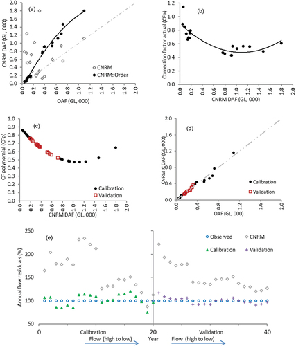
In step 4: CFp for the 25th to 75th percentile DAF of CNRM is calculated using the previous polynomial equation for validation purposes. These CFp for validation are plotted along with the CFp of the top and bottom 25th percentile of DAF of CNRM used in calibration (Fig. 4(c)). The CFp for calibration and validation are used to correct DAF of CNRM for the top and bottom 25th percentile (utilized in calibration) and the 25th to 75th percentile (adopted for validation), respectively. The corrected DAF values for CNRM (CNRM: C DAF) are plotted against the CNRM DAF values before correction to depict the relationship before and after correction (Fig. 4(d)). The $CNRMDA{F}_c$ shows a non-linear (polynomial) relationship with the CNRM DAF (as corrected flows, which were corrected using a 2^nd order polynomial, align closely with the 1:1 line).

The CFp for the top and bottom 25th percentile of DAF for CNRM are calculated using the polynomial equation and applied to correct corresponding DAF. This demonstrates a close alignment of DAF_c for CNRM to 1:1 line (Fig. 4(d)) and represents a good fit of DAF_c with OAF. The statistical measures of calibration and validation of the method for all GCMs are summarized in Table 2. The value of NSE for the calibration period for CNRM was improved from −0.84 to 0.97. The CC appeared not to be a good measure here, because the model tends to predict with good correlation before and after correction for both calibration and validation period. The E value shows that DAF was 83% higher compared to the OAF before calibration, which comes to zero with calibration. Similar to calibration, the values of NSE and E were also improved for validation for the DAF. The value of NSE was improved from −1.06 to 0.98, and E improved from 57% over-prediction to close to zero.

Results in Table 2 reveal that in all cases for every GCM, the NSE improved considerably but varied in a wide range. For example, values of NSE for CNRM, CSIRO, IPSL, MIROC and MPI have improved dramatically (>200%) and significant improvement occurred for CCM (135%), while for other GCMs the value has improved reasonably (10–31%). The E values are closely matched to zero in all cases for every GCM for the calibration period. Similar to calibration, the NSE value improved for almost all cases for every GCM, except for CCM and GISSR where NSE remains close to the value before validation. In addition, the E value improved significantly for most GCMs, except CCM, CSIRO, CSIRO2, GISSR and MPI where E values are already close to zero before validation and remained similar after validation with only slight variation. The annual flow residuals for the calibration and validation period of DAF and DAF_c for CNRM is presented in Fig. 4(e), where OAF is considered 100%. It is observed that DAF values in some years are more than double the OAF values for both calibration and validation periods, and they over-predict in every year except one. It is also evident that the DAF_c closely matches OAF in most cases, with little residual flow for both the calibration and validation periods.

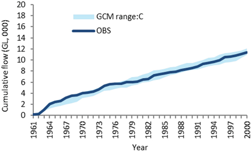
A comparative summary of DAF and DAFc (obtained through calibration and validation) along with OAF is presented in Fig. 5. The distribution of cumulative DAF_c for the 11 GCMs for the hindcast period achieved through calibration and validation was compared to the distribution of OAF values (Fig. 5). It was revealed that the distribution of DAF_c closely matches the distribution of OAF. The distribution of DAF before and after correction (through calibration and validation) is also presented (Fig. 5) to demonstrate the level of correction achieved through the calibration and validation for each of the GCMs. In addition, a cumulative plot of DAF, DAF_c and OAF for the hindcast period provides evidence of better goodness of fit of DAF_c with OAF, denoting the correction of DAF as appropriate (for each GCM; see Fig. 5). Therefore, it is evident that the bias correction method can reduce biases in the final form of DAF, although different levels of bias may be prevalent in different GCMs initially.

Figure 5. Corrected DAFc for 11 GCMs for the hindcast period (1961–2000) which covers both calibration and validation periods. The ranges of cumulative DAF and DAFc for 11 GCMs are summarized with observed annual flow for the hindcast period where DAFc was achieved through the calibration and validation process.

3.3 Correction of future projections of GCM DAF

The bias correction method is applied to correct the future projections of GCM DAF for two emission scenarios A2 and B1 for mid (2046–2065) and late (2081–2100) century. This process is similar to step 4 used for calibration but it assumes the polynomial relationship (CFp) from the hindcast remains the same for the future simulation. This assumption may be reasonable as the bias may remain unchanged. This is because the observed and modelled statistics of current climate are used to adjust the model output for the future period (Johnson and Sharma 2012). Measurement of the reduction in the extreme value of DAF using standard deviation (STD) delineates an improved distribution of DAF data achieved through the bias correction. A summary of mean DAF and STD as projected by the 11 GCMs (corrected and uncorrected) for the mid (2046–2064) and late (2081–2100) century under scenarios A2 and B1 at Baden Powell gauging station is presented in Table 3. In most cases, the STD of DAF_c was found to be smaller compared to the STD of DAF before correction, particularly for high flows. This indicates a greater central tendency of DAFc compared to DAF before correction. The STD of higher values showing greater reduction after correction means high flow was corrected to a greater extent compared to lower flow, which is consistent with the biases observed for the hindcast period. For example, STD values decreased by a greater amount from values around 100 or higher for both scenarios (A2 and B1) during the middle and end of this century.

Table 3. Mean and standard deviation (STD) of DAF and corrected DAF (GL) for 11 GCMs for scenarios A2 and B1 during the mid (2046–2065) and late century (2081–2100) at Baden Powell gauging station.

			CCM	CNRM	CSIRO	CSIRO2	GFDL1	GFDL2	GISSR	IPSL	MIROC	MPI	MRI	ENS
Scenario: A2	2046–2065	Mean	156	135	124	330	212	61	88	553	61	130	297	195
		Mean:C	135	93	145	309	160	62	106	399	79	133	236	169
		STD	253	168	85	309	229	61	57	391	36	140	255	68
		STD:C	170	96	89	277	186	55	62	340	44	113	201	51
	2081–2100	Mean	62	39	168	182	40	27	49	148	46	47	58	79
		Mean:C	63	32	169	179	31	28	60	124	56	59	49	77
		STD	47	37	196	157	35	40	58	129	63	41	33	29
		STD:C	47	30	129	117	26	39	62	82	69	47	27	20
Scenario: B1	2046–2065	Mean	183	239	90	196	278	111	171	429	189	213	219	211
		Mean:C	172	146	104	193	201	100	176	287	170	190	178	174
		STD	144	294	99	162	184	151	216	300	241	205	190	75
		STD:C	126	142	101	110	134	112	183	173	111	144	161	49
	2081–2100	Mean	103	177	179	346	249	52	83	304	103	159	350	191
		Mean:C	101	121	187	304	185	52	102	231	105	169	273	166
		STD	103	178	149	207	208	63	50	248	155	111	182	52
		STD:C	95	100	130	138	166	56	52	142	86	99	139	39

ENS: ensemble. Mean is for a 20-year period. Mean:C is the corrected mean for the 20-year period. Values are in GL.

In determining the state of biases of DAF for the hindcast period (1961–2000), we found that the DAF for a particular GCM has a tendency to generate high values in some years that bear little relation to the OAF in those years (Fig. 3(a)). The STD values of 100 or less remained similar after correction of DAF. We also discerned that STD values for some of the low flow values increased after correction, indicating low flow is corrected to higher values. The level of correction for an individual GCM is dependent on the level of biases demonstrated during the hindcast period (which was captured in correction factors) and also the level of bias for the projected periods under the scenarios (A2 and B1). Hence, it is expected that there should not be a particular trend or relationship between STD values of corrected and uncorrected DAF among the GCMs, as the levels of bias are independent for different GCMs. The reduction in STD for corrected DAF for high flows indicates the correction with greater central tendency.

The correction of DAF measured as a 20-year mean (relative to the corresponding mean before correction) produces mixed results (increase, same or decrease) for the two scenarios (A2 and B1) during the mid and late century for different GCMs, with an overall decrease of the ensemble mean after correction (see Table 3). For example, mean DAF corrected to lower values for CCM, CNRM, CSIRO2, GFDL1, IPSL and MRI while it corrected higher for CSIRO, GFDL2, GISSR, MIROC and MPI, resulting in an overall decrease for the ensemble mean from 195 to 169 GL for mid-century under scenario A2 (Table 3). A similar nature of correction is observed under scenarios A2 and B1 resulting in a decrease of the corresponding ensemble mean from 79 to 77 GL and from 191 to 166 GL during the late and mid-century, respectively. The corrected DAF for the majority of the GCMs manifests a decrease (except for CSIRO and GISSR) under the scenario B1 during mid-century, with the corrected ensemble mean of DAF decreasing from 211 to 174 GL. Mean DAF is generally corrected to increase for CSIRO, GFDL2, GISSR, MIROC and MPI for the mid- and late century under scenario A2, and the same is also true for the late century under scenario B1 – except with GFDL2, for which the corrected DAF remains the same. The mean DAF values are corrected to increase only for CSIRO and GISSR for mid-century under scenario B1, while for other GCMs mean DAF values decrease after correction.

The changes in STD values provide a measure of correction in the distribution of DAF data before and after correction. For example, although the mean DAF for GFDL2 increased from 61 to 62 GL for mid-century under scenario A2, the corresponding STD values were corrected to decrease from 61 to 55, indicating a greater central tendency of DAF_c compared to DAF before correction (Table 3). The same is also noted for GISSR during the mid-century under scenario B1, where the mean DAF is corrected to increase from 171 to 176 GL with a decrease in corrected STD values from 216 to 183. Therefore, DAF_c values in all cases are more centrally distributed compared to DAF (before correction). A narrow (or a more central) distribution of DAF_c (relative to the distribution of DAF) is a measure of reduced biases obtained through the application of this bias correction method.

3.4 Effect of bias correction on the cumulative annual flow

Another approach for measuring reduction of biases is plotting the projected and corrected DAF data in a cumulative distribution. The range of cumulative values of DAF in the 20-year projected period for the mid (2046–2065) and late (2081–2100) century were corrected and are presented in Fig. 6 for both scenarios. The results revealed that the cumulative annual flow has been corrected significantly, except for A2 in late century. The DAF ensemble mean from the 11 GCMs has been corrected to lower values. The cumulative flow range of DAF over 20 years is corrected from approximately 8600~1800 GL to 5700~2000 GL under the B1 scenario during mid this century. Similarly, the cumulative ensemble mean of DAF was corrected from approximately 4200 GL to 3500 GL under scenario B1 during mid-century (Fig. 6(b)). Thus, the DAF range is reduced by 46% after correction. Similar to scenario B1 during mid-century, the range of DAF was corrected from approximately 11000~1200 GL to 8000~1200 GL for scenario A2 during the mid-century, showing a large reduction (by approximately 3000 GL) in range, which is approximately 30% lower relative to the range (9800 GL) before correction.

Figure 6. Cumulative distribution of DAF before and after correction as represented by 11 GCMs during the mid and late century under scenarios A2 and B1. The corresponding ensemble means of DAF for 11 GCMs are also presented before and after correction. The GCM range represents the maximum and minimum GCM DAF in the ensemble of 11 GCMs for the projected period, while the GCM range:C means the same after bias correction. Cum:Avg. represents the cumulative ensemble mean of 11 GCMs’ DAF for the projected period, while Cum:Avg:C means the same after bias correction.

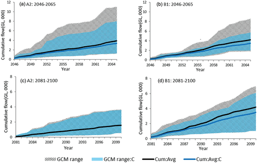
The cumulative distribution of DAF during the late century (2081–2100) under both A2 and B1 scenarios shows that the distribution has a relatively narrower range (Fig. 6(c) and (d)). The range of DAF was corrected from approximately 7000~1000 GL to 6000~1000 GL, resulting in a reduced range after correction by approximately 17% compared to the range (6000 GL) before correction under scenario B1 during the late century. The correction of the range of DAF for scenario A2 during the late century is relatively insignificant compared to the other three cases (A2 mid-century, B1 mid-century and B1 late century). More specifically, the range of DAF corrected from 3642~547 GL to 3581~568 GL still reduces the range by 81 GL which is a reduction of approximately 3% compared to the range (3095 GL) before correction for scenario A2 during the late century.

The reason for the lower degree of correction for scenario A2 during the late century is that the projected DAF is relatively low compared to the other scenario. It was found from the calibration that the GCM DAF has an upward bias in most cases, particularly for high flow, and as a result, greater correction applies to high flow with correction factors ranging from 0.6 to 0.9, while in most cases for low flow the correction factors are usually close to 1.0. The DAF for scenario A2 during the late century is relatively low, and this indicates that the correction factors in most of the cases applied to correct individual DAF data were close to 1, resulting in little correction, which is consistent with the principle of this bias correction method.

3.5 Runoff changes before and after bias correction

In a previous study (Islam et al. 2014), significant bias was observed for the future projections of GCM-derived runoff (streamflow) for the Murray-Hotham catchment in SWWA. The bias reported in that study was considered here, and the changes in runoff before and after applying this bias correction method are shown in Table 4. The comparison of changes in runoff at Baden Powell gauging station before and after correction during the mid and late century under A2 and B1 scenario shows some significant changes in runoff changes values after application of this bias correction method. The results revealed that the ensemble mean of DAF for all four cases has been corrected better. It should be noted that the ensembles of both high (90th percentile) and median (50th percentile) flow are corrected to reduce further while the ensemble of low flow (10th percentile) is corrected to increase in all cases.

Table 4. Comparison of reduction of runoff and corrected reduction of runoff for the ensemble mean of 11 GCMs for scenarios A2 and B1 for mid- and late century. Values in parentheses (taken from Islam et al. 2014) represent runoff reduction before the correction method is applied.

Gauging stations	Percentile	Observed runoff (GL)				Change in average runoff with respect to the past (%)*
		Historical (1961–2000)	Past (1961–1980)	Recent (1981–2000)	Change (%)	2046–2065		2081–2100
						A2	B1	A2	B1
Baden Powell	Q90	537	692	389	−44	−52(−40)	−50(−35)	−78(−77)	−59(−50)
	Q50	220	233	210	−10	−50(−43)	−46(−41)	−76(−79)	−38(−34)
	Q10	92	85	114	34	−49(−54)	−30(−34)	−76(−80)	−30(−34)
	Mean	285	307	264	−14	−45(−36)	−43(−31)	−75(−74)	−46(−38)

*increase (+), decrease (−).

4 Discussion

For many different planning purposes, we need to predict future rainfall and streamflow; these can be deduced using GCM data, but the process involves uncertainty. This uncertainty remains with the embedded procedure of the forecasting system. For example, Huttner (2020) reported that a seven-day forecast can accurately predict the weather about 80% of the time while a five-day forecast can predict accurately approximately 90% of the time. It is more challenging to predict weather accurately 7–14 days in advance and there will be more inaccuracy in a longer-term forecast. When it comes to climate models, GCMs have improved their performance over time, with greater resolution from CMIP3 to CMIP5 to CMIP6, and they are expected to continue to improve in future releases, but this does not provide bias-free simulation (Tian and Dong 2020). For longer-term projections of future climate, the reliability of simulation may decrease with increased uncertainties.

To address uncertainties, a multi-model ensemble approach is widely used to generate plausible scenarios for the future hydrological regime (Christensen and Lettenmaier 2007, Bari et al. 2010, Islam et al. 2014, Haque et al. 2015, Woznicki et al. 2016). Although the ensemble approach involves significant uncertainties, it provides a range of plausible future changes in the hydrological regime in a catchment. For example, in two similar studies, it was found that the flow is projected to increase (compared to the observed past) in the Ord River catchment (Islam et al. 2011) while flow is projected to decrease in the Murray-Hotham River catchment (Islam et al. 2014) during mid (2046–2065) and late (2081–2100) century under scenarios A2 and B1. Hence, ensembles of flow generated by a combination of GCMs provide a better picture of possible future change and variability of the flow regime in a catchment. These plausible future scenarios of rainfall and runoff changes in a catchment due to climate change could be useful for water resources managers and policymakers (Coulibaly 2009). For water resources management, managers are more interested in assessing changes in streamflow at the catchment scale during the next 50 to 100 years for planning purposes. This is because many water structures are designed for a 100-year return period. Therefore, it is very important to assess the effect of climate change on water resources for future projections of water availability. This information would be very beneficial for planning future water supply sources or searching for alternative water sources and making investments to meet future water demand considering the possible uncertainties.

These uncertainties may be reduced by the use of the bias correction method presented in this paper. The method developed in this study reduces the biases of the final product (here, DAF) in a holistic way, which means it reduces bias irrespective of its sources (e.g. from the GCM, downscaling method or hydrological model). Another advantage of this approach is that it does not require tracking down the propagation and intermingling of biases through the process of hydrological assessment of climate change; rather, it reduces biases in the end product (i.e. DAF). Hence, this method may be applicable for any number and combination of ensemble members (such as a number of GCMs, downscaling methods and hydrological models) without modification.

Although the bias correction method was applied using AR4 GCM data from the IPCC to check the improvement of runoff changes in Murray-Hotham catchment against that of Islam et al. (2014), the method presented herein is applicable for any IPCC assessment report GCM data, such as AR5 (CMIP5) data for different RCPs and/or AR6 (CMIP6) data for different SSPs. The hindcast of AR4 data used in this study was for 1961–2000, but one can use AR5/AR6 data for the recent hindcast. Whatever the data used for bias correction, the hindcast data can be used for calibration (using the top and bottom 25th percentile hindcast data) and validation (using the 25th–75th percentile hindcast data), and the validation procedure can be used to correct the future simulation. Having the correct future simulation data is very important for the planning of future infrastructure development of a country.

5 Conclusions

A bias correction method based on a polynomial correction factor was developed in this study to reduce bias in GCM DAF values at the catchment scale. The method was applied to correct GCM DAF for the Murray-Hotham catchment in Western Australia for the mid (2046–2065) and late (2081–2100) century under the scenarios A2 and B1. The method is calibrated and validated using DAF and OAF for the hindcast period (1961–2000). The correction factors derived for individual GCMs through the calibration process are used to correct the DAF for the two scenarios. The calibration and validation statistics (such as NSE and E) indicate that the method is well calibrated and validated. Therefore, the method is capable of correcting bias of DAF for the projected periods under the climate scenarios considering the polynomial relationship of the hindcast remains the same for the future simulation.

Correction of maximum flow to lower values, and minimum values to higher values, improving the distribution of DAF towards central values (measured as standard deviation), and reducing the range of cumulative flow over a 20-year time period, all show bias reduction. The relationship between decadal rainfall and runoff for the observed and projected periods, for scenarios A2 and B1, at a gauging station in the catchment was presented in Islam et al. (2014); this has been corrected in the present study for the flow (runoff) changes for the projected periods. This shows the relationship between DAF and corrected DAF (runoff) changes on a decadal scale, which can be used to estimate the corrected DAF for any identified changes of DAF. The corrected decadal DAF changes could be useful to water resources managers or policymakers in planning future water resources. Hence, the results of DAF changes (runoff changes) deduced with the extended relationships are expected to represent better estimates of future changes of runoff in the catchment as depicted by the GCMs under the two scenarios. This bias correction of the DAF reduces the bias of the end product (runoff) considering the total bias generated from the GCM output, downscaling and/or hydrological modelling.

Acknowledgements

This study is part of a PhD research project carried out by the first author at Curtin University, Western Australia. The initial stage of this PhD research project was supported by a scholarship grant (Australian Postgraduate Award, Australian Government) awarded to the first author. The authors acknowledge the data support of the Bureau of Meteorology, Australian Government, and Department of Water and Environmental Regulation, Government of Western Australia. The authors also thank the reviewer and associate editor for providing professional comments on the first draft which improved the quality of this paper.

Disclosure statement

No potential conflict of interest was reported by the author(s).

Appendix

Figure A1. The GCM-derived annual flow values for 11 GCMs are plotted against the corresponding observed annual flow for the hindcast period at Baden Powell gauging station.

Figure A1. (Continued).

References

- Ahmed, K., et al., 2019. Selection of multi-model ensemble of general circulation models for the simulation of precipitation and maximum and minimum temperature based on spatial assessment metrics. Hydrology and Earth System Sciences, 23, 4803–4824. doi:10.5194/hess-23-4803-2019.
- Anwar, A.H.M., et al., 2011. The effect of climate change on stream flow reduction in Murray-Hotham river catchment, Western Australia. IWA water convention conference-sustainable water solutions for a changing urban environment, 4–8 July. Singapore: Singapore International Water Week.
- Bae, D.-H., Jung, I.-W., and Lettenmaier, D.P., 2011. Hydrologic uncertainties in climate change from IPCC AR4 GCM simulations of the Chungju Basin, Korea. Journal of Hydrology, 401 (1–2), 90–105. doi:10.1016/j.jhydrol.2011.02.012.
- Bari, M.A., Amirthanathan, G.E., and Timbal, B. 2010 Climate change and long term water availability in South-Western Australia - an experimental projection. Climate change 2010: practical responses to climate change national conference, 29–1 September–October. Melbourne, Australia. Available from: https://search.informit.com.au/documentSummary;dn=769270460134136;res=IELENG.
- Bari, M.A., Shakya, D.M., and Owens, M., 2009. LUCICAT Live – A modelling framework for predicting catchment management options, In: R.S. Anderssen, R.D. Braddock, and L.T.H. Newham (eds.) 18th World IMACS Congress and MODSIM09 International Congress on Modelling and Simulation. Modelling and Simulation Society of Australia and New Zealand and International Association for Mathematics and Computers in Simulation, July , 3457-3463. https://mssanz.org.au/modsim09/I8/bari.pdf
- Bari, M.A. and Smettem, K.R.J., 2003. Development of a salt and water balance model for a large partially cleared catchment. Australasian Journal of Water Resources, 7 (2), 93–99. doi:10.1080/13241583.2003.11465232.
- Blöschl, G. and Sivapalan, M., 1995. Scale issues in hydrological modelling: a review. Hydrological Processes, 9, 251–290. doi:10.1002/hyp.3360090305.
- Chen, J., et al., 2011. Overall uncertainty study of the hydrological impacts of climate change for a Canadian watershed. Water Resources Research, 47 (12), 1–16. doi:10.1029/2011WR010602.
- Christensen, N.S. and Lettenmaier, D.P., 2007. A multimodel ensemble approach to assessment of climate change impacts on the hydrology and water resources of the Colorado River Basin, Hydrol. Hydrology and Earth System Sciences, 11, 1417–1434. doi:10.5194/hess-11-1417-2007.
- Coulibaly, P., 2009. Multi-model approach to hydrologic impact of climate change, and Taniguchi, et al., eds. From headwaters to the ocean, hydrological change and water management. London: CRC Press, Taylor and Francis Group, 249–255.
- Demirel, M.C., et al., 2018. Combining satellite data and appropriate objective functions for improved spatial pattern performance of a distributed hydrologic model. Hydrology and Earth System Sciences, 22, 1299–1315. doi:10.5194/hess-22-1299-2018.
- Dibike, Y.B. and Coulibaly, P., 2005. Hydrologic impact of climate change in the Saguenay watershed: comparison of downscaling methods and hydrologic models. Journal of Hydrology, 307 (1–4), 145–163. doi:10.1016/j.jhydrol.2004.10.012.
- Ehret, U., et al., 2012. HESS Opinions “Should we apply bias correction to global and regional climate model data?” Hydrology and Earth System Sciences, 16 (9), 3391–3404. doi:10.5194/hess-16-3391-2012.
- Evans, J.P., et al., 2014. Design of a regional climate modeling projection ensemble experiment. NARCliM. Geoscience Model Development, 7, 621–629. doi:10.5194/gmd-7-621-2014.
- Fita, L., et al., 2016. Evaluation of the regional climate response in Australia to large-scale climate models in the historical NARCliM simulations. Climate Dynamics, 1, 2815–2829. doi:10.1007/s00382-016-3484-x.
- Ghosh, S. and Mujumdar, P.P., 2007. Nonparametric methods for modeling GCM and scenario uncertainty in drought assessment. Water Resources Research, 43 (7), 1–19. doi:10.1029/2006WR005351.
- Ghosh, S. and Mujumdar, P.P., 2009. Climate change impact assessment: uncertainty modeling with imprecise probability. Journal of Geophysical Research, 114 (18), D18113. doi:10.1029/2008JD011648.
- Haddeland, I., et al., 2012. Effects of climate model radiation, humidity and wind estimates on hydrological simulations. Hydrology and Earth System Sciences, 16, 305–318. doi:10.5194/hess-16-305-2012.
- Hagemann, S., et al., 2011. Impact of a statistical bias correction on the projected hydrological changes obtained from three GCMs and two hydrology models. Journal of Hydrometeorology, 12 (4), 556–578. doi:10.1175/2011JHM1336.1.
- Haque, M., et al., 2015. Estimation of catchment yield and associated uncertainties due to climate change in a mountainous catchment in Australia. Hydrological Processes, 29 (19), 4339–4349. doi:10.1002/hyp.10492.
- Hempel, S., et al., 2013. A trend-preserving bias correction – the ISI-MIP approach. Earth System Dynamics, 4, 219–236. doi:10.5194/esd-4-219-2013.
- Henriksen, H.J., et al., 2008. Assessment of exploitable groundwater resources of Denmark by use of ensemble resource indicators and a numerical groundwater–surface water model. Journal of Hydrology, 348, 224–240. doi:10.1016/j.jhydrol.2007.09.056.
- Hossain, M.M., et al., 2021a. Comparing spatial interpolation methods for CMIP5 monthly precipitation at catchment scale. Indian Water Resources Society, 41 (2), 28–34. Available from: http://iwrs.org.in/journal/apr2021/5apr.pdf.
- Hossain, M.M., et al., 2021b. Drift in CMIP5 decadal precipitation at catchment level. Stochastic Environmental Research and Risk Assessment. doi:10.1007/s00477-021-02140-8.
- Hossain, M.M., et al., 2021c. Intercomparison of drift correction alternatives for CMIP5 decadal precipitation. International Journal of Climatology. doi:10.1002/joc.7287.
- Hughes, D.A., Kingston, D.G., and Todd, M.C., 2011. Uncertainty in water resources availability in the Okavango River basin as a result of climate change. Hydrology and Earth System Sciences, 15 (3), 931–941. doi:10.5194/hess-15-931-2011.
- Huttner, P. 2020. How accurate are forecast models 1 to 2 weeks ahead? Forecast models keep hinting at subzero air by mid-January. MPRnews, 2 Jan. Available from: https://www.mprnews.org/story/2020/01/02/forecast-models-keep-hinting-at-subzero-air-ahead [ Accessed 22 November 2022].
- Ines, A.V.M. and Hansen, J.W., 2006. Bias correction of daily GCM rainfall for crop simulation studies. Agricultural and Forest Meteorology, 138, 44–53. doi:10.1016/j.agrformet.2006.03.009.
- Intergovernmental Panel on Climate Change (IPCC). 2000. Special report on emission scenarios. UK: Cambridge University Press, 570. Available from: https://www.ipcc.ch/site/assets/uploads/2018/03/emissions_scenarios-1.pdf.
- Intergovernmental Panel on Climate Change (IPCC). 2007 Climate change 2007: impacts, adaptation, and vulnerability: working group II contribution to the intergovernmental panel on climate change fourth assessment report, summary for policymakers, Cambridge, UK: Cambridge University Presss, 7–22. Available from: https://www.ipcc.ch/site/assets/uploads/2018/02/ar4-wg2-spm-1.pdf.
- Islam, S.A., Bari, M., and Anwar, A.H.M.F. 2011 Assessment of hydrologic impact of climate change on Ord river catchment of Western Australia for water resources planning: a multi-model ensemble approach. Proceedings of the 19th International Congress on Modelling and Simulation, 12–16 December 2011. Perth, Western Australia, 3587–3593. Available from: https://www.mssanz.org.au/modsim2011/I6/islam.pdf.
- Islam, S.A., Bari, M.A., and Anwar, A.H.M.F., 2014. Hydrologic impact of climate change on Murray-Hotham catchment of Western Australia: a projection of rainfall-runoff for future water resources planning. Hydrology and Earth System Sciences, 18 (9), 3591–3614. doi:10.5194/hess-18-3591-2014.
- Johnson, F. and Sharma, A., 2011. Accounting for interannual variability: a comparison of options for water resources climate change impact assessments. Water Resources Research, 47 (4). doi:10.1029/2010WR009272.
- Johnson, F. and Sharma, A., 2012. A nesting model for bias correction of variability at multiple time scales in general circulation model precipitation simulations. Water Resources Research, 48, W01504. doi:10.1029/2011WR010464.
- Krause, P., Boyle, D.P., and Bäse, F., 2005. Comparison of different efficiency criteria for hydrological model assessment. Advances in Geosciences, 5, 89–97. doi:10.5194/adgeo-5-89-2005.
- Kundzewicz;, Z.W., et al., 2007. Freshwater resources and their management. Climate change 2007: impacts, adaptation and vulnerability – contribution of working group II to the fourth assessment report of the Intergovernmental Panel on Climate Change. Cambridge, UK and New York, NY, USA: Cambridge University Press. Available from: https://www.ipcc.ch/site/assets/uploads/2018/02/ar4-wg2-chapter3-1.pdf.
- Laflamme, E.M., Linder, E., and Pan, Y., 2016. Statistical downscaling of regional climate model output to achieve projections of precipitation extremes. Weather and Climate Extremes, 12, 15–23. doi:10.1016/j.wace.2015.12.001.
- Lenderink, G., Buishand, A., and van Deursen, W., 2007. Estimates of future discharges of the river Rhine using two scenario methodologies: direct versus delta approach. Hydrology and Earth System Sciences, 11 (3), 1145–1159. doi:10.5194/hess-11-1145-2007.
- Maraun, D., 2016. Bias correcting climate change simulations—a critical review. Current Climate Change Reports, 2, 211–220. doi:10.1007/s40641-016-0050-x.
- Maraun, D., et al., 2010. Precipitation downscaling under climate change: recent developments to bridge the gap between dynamical models and the end user. Reviews of Geophysics, 48 (2009RG000314), 1–38. doi:10.1029/2009RG000314.
- Mehan, S., Gitau, M.W., and Flanagan, D.C., 2019. Reliable future climatic projections for sustainable hydro-meteorological assessments in the Western Lake Erie Basin. Water, 11 (3), 581. doi:10.3390/w11030581.
- Mehrotra, R. and Sharma, A., 2015. Correcting for systematic biases in multiple raw GCM variables across a range of timescales. Journal of Hydrology, 520, 214–223. doi:10.1016/j.jhydrol.2014.11.037.
- Mehrotra, R. and Sharma, A., 2016. A multivariate quantile-matching bias correction approach with auto- and cross-dependence across multiple time scales: implications for downscaling. Journal of Climate, 29, 3519–3539. doi:10.1175/JCLI-D-15-0356.1.
- Muerth, M.J., et al., 2013. On the need for bias correction in regional climate scenarios to assess climate change impacts on river runoff. Hydrology and Earth System Sciences, 17 (3), 1189–1204. doi:10.5194/hess-17-1189-2013.
- New, M. and Hulme, M., 2000. Representing uncertainty in climate change scenarios: a Monte-Carlo approach. Integrated Assessment, 1 (3), 203–213. doi:10.1023/A:1019144202120.
- Nishant, N., et al., 2021. Introducing NARCliM1.5: evaluating the performance of regional climate projections for southeast Australia for 1950–2100. Earth’s Future, (9), e2020EF001833. doi:10.1029/2020EF001833.
- Nóbrega, M.T., et al., 2011. Uncertainty in climate change impacts on water resources in the Rio Grande Basin, Brazil. Hydrology and Earth System Sciences, 15, 585–595. doi:10.5194/hess-15-585-2011.
- Piani, C., Haerter, J.O., and Coppola, E., 2010. Statistical bias correction for daily precipitation in regional climate models over Europe. Theoretical and Applied Climatology, 99 (1–2), 187–192. doi:10.1007/s00704-009-0134-9.
- Randall, D.A., et al., 2007. Climate models and their evaluation. Climate change 2007: the physical science Ba-sis, contribution of working group I to the Fourth Assessment Report of the Intergovernmental Panel on Climate Change. Cambridge, UK and New York, NY, USA: Cam-bridge University Press. Available from: https://www.ipcc.ch/site/assets/uploads/2018/02/ar4-wg1-chapter8-1.pdf.
- Rojas, R., et al., 2011. Improving pan-European hydrological simulation of extreme events through statistical bias correction of RCM-driven climate simulations. Hydrology and Earth System Sciences, 15, 2599–2620. doi:10.5194/hess-15-2599-2011.
- Semenov, M.A. and Barrow, E.M. 2002 LARS-WG: a stochastic weather generator for use in climate impact studies, Version 3.0, user manual. Available from: http://resources.rothamsted.ac.uk/sites/default/files/groups/mas-models/download/LARS-WG-Manual.pdf.
- Shams, M.S., et al., 2018. Relating ocean-atmospheric climate indices with Australian river streamflow. Journal of Hydrology, 556, 294–309. doi:10.1016/j.jhydrol.2017.11.017.
- Sunyer, M.A., Madsen, H., and Ang, P.H., 2012. A comparison of different regional climate models and statistical downscaling methods for extreme rainfall estimation under climate change. Atmospheric Research, 103, 119–128. doi:10.1016/j.atmosres.2011.06.011.
- Surfleet, C.G., et al., 2012. Selection of hydrologic modeling approaches for climate change assessment: a comparison of model scale and structures. Journal of Hydrology, 464–465, 233–248. doi:10.1016/j.jhydrol.2012.07.012.
- Teutschbein, C. and Seibert, J., 2010. Regional climate models for hydrological impact studies at the catchment scale: a review of recent modeling strategies. Geography Compass, 7, 834–860. doi:10.1111/j.1749-8198.2010.00357.x.
- Teutschbein, C. and Seibert, J., 2012. Bias correction of regional climate model simulations for hydrological climate-change impact studies: review and evaluation of different methods. Journal of Hydrology, 456-457, 12–29. doi:10.1016/j.jhydrol.2012.05.052.
- Tian, B. and Dong, X., 2020. The double‐ITCZ Bias in CMIP3, CMIP5 and CMIP6 models based on annual mean precipitation. Geophysical Research Letters, 47, e2020GL087232. doi:10.1029/2020GL087232.
- Timbal, B., Fernandez, E., and Li, Z., 2009. Generalization of a statistical downscaling model to provide local climate change projections for Australia. Environmental Modelling and Software, 24, 341–358. doi:10.1016/j.envsoft.2008.07.007.
- Wilby, R.L., et al., 2004. Guidelines for use of climate scenarios developed from statistical downscaling methods. Available from: http://www.narccap.ucar.edu/doc/tgica-guidance-2004.pdf [Accessed 16 June 2016].
- Wilby, R.L., Dawson, C.W., and Barrow, E.M., 2002. SDSM — a decision support tool for the assessment of regional climate change impacts. Environmental Modelling and Software, 17 (2), 145–157. doi:10.1016/S1364-8152(01)00060-3.
- Wilby, R.L. and Harris, I., 2006. A framework for assessing uncertainties in climate change impacts: low-flow scenarios for the River Thames, UK. Water Resources Research, 42 (2), W02419. doi:10.1029/2005WR004065.
- Wood, A.W., et al., 2004. Hydrologic implications of dynamical and statistical approaches to downscaling climate model outputs. Climatic Change, 62, 189–216. doi:10.1023/B:CLIM.0000013685.99609.9e.
- Woznicki, S.A., et al., 2016. Large-scale climate change vulnerability assessment of stream health. Ecological Indicators, 69, 578–594. doi:10.1016/j.ecolind.2016.04.002.