Exploring the potential of the dynamic hysteresis loops via high field, high frequency and temperature adjustable AC magnetometer for magnetic hyperthermia characterization

Abstract

Aim

The Specific Absorption Rate (SAR) is the key parameter to optimize the effectiveness of magnetic nanoparticles in magnetic hyperthermia. AC magnetometry arises as a powerful technique to quantify the SAR by computing the hysteresis loops' area. However, currently available devices produce quite limited magnetic field intensities, below 45mT, which are often insufficient to obtain major hysteresis loops and so a more complete and understandable magneticcharacterization. This limitation leads to a lack of information concerning some basic properties, like the maximum attainable (SAR) as a function of particles' size and excitation frequencies, or the role of the mechanical rotation in liquid samples.

Methods

To fill this gap, we have developed a versatile high field AC magnetometer, capable of working at a wide range of magnetic hyperthermia frequencies (100 kHz – 1MHz) and up to field intensities of 90mT. Additionally, our device incorporates a variable temperature system for continuous measurements between 220 and 380 K. We have optimized the geometrical properties of the induction coil that maximize the generated magnetic field intensity.

Results

To illustrate the potency of our device, we present and model a series of measurements performed in liquid and frozen solutions of magnetic particles with sizes ranging from 16 to 29 nm.

Conclusion

We show that AC magnetometry becomes a very reliable technique to determine the effective anisotropy constant of single domains, to study the impact of the mechanical orientation in the SAR and to choose the optimal excitation parameters to maximize heating production under human safety limits.

Keywords:

• AC magnetometry
• specific absorption rate
• SAR
• magnetic hyperthermia
• stoner–Wohlfarth model based theories

1. Introduction

Magnetic hyperthermia (MH) is an important novel therapy, which consists in damaging and destructing cancer cells increasing the temperature of the tumors up to 41–46° C [1–6]. The MH is induced diffusing magnetic nanoparticles (MNPs) into the tumor tissue and then irradiating this area with an alternating magnetic field (AMF) with a frequency ranging between 100 kHz and 1 MHz. Under such conditions, magnetic nanoparticles act as very local heat sources, which are capable of rising the temperature of tumors while leaving the healthy tissues basically undamaged.

The indispensable initial step for designing a successful hyperthermia therapy is to determine the specific absorption rate (SAR) of the MNPs, which is the absorbed energy per unit of nanoparticle mass. This parameter greatly depends on the physicochemical properties of the nanoparticles such as composition, size, shape, crystallinity, saturation magnetization, etc [7–9]. Additionally, interparticle magnetic interactions and the interplay between particles and biological systems also affect the heating performance of MNPs [10,11]. To avoid collateral damages in the hyperthermia treatment, the applied magnetic field and frequency as well as the injected MNP amount should be minimized. Therefore, it is essential to count on MNP system with optimal SAR values, but even more fundamental is to gain knowledge about what characteristics of the system are really significant in order to score these optimal values. For instance, some SAR values reported so far in the literature are very high [12,13] but it is unclear if such rates rely entirely on particles-dependent properties (as the composition, size or shape) or also on the way in which these particles are assembled within the colloid. In order to find the best potential candidates for magnetic hyperthermia, an accurate understanding of the physical effects involved in the heat production is as important as the final values of SAR obtained in a given experiment.

Vast majority of SAR measurements reported in the literature are obtained from calorimetry methods, by directly measuring the increase of temperature as functions of time when MNPs are exposed to AMF [13–19]. Ultimately, the heat production of MNPs caused by AC magnetic fields is originated by the hysteretic dynamic response of these MNPs to the AC excitation, so the direct determination of this hysteresis by AC magnetometry is a powerful alternative to calorimetry in determining the SAR [17,20–22]. In general, both techniques are highly complementary, as discussed elsewhere [21,23], considering that there are several factors that can downgrade the accuracy of SAR values obtained from temperature versus time measurements [24]. Indeed, AC magnetometry provides additional and very valuable magnetic information that is not directly accessible by calorimetry alone. For instance, collective phenomena of MNPs, related to the type of assembling, disordered or forming well-defined structures, are easily detected from the AC hysteresis loop [25–29]. AC magnetometry has also allowed to correlate the shape of the MNPs and their hyperthermia performance [30], or to clarify why the heating power of MNPs tends to fall in cellular enviroments [31]. In addition, AC magnetometry studies have made possible the development of new coating strategies to keep constant the heating performance of MNPs in media with different viscosities and ionic strength [32].

In recent years several home-made and commercial AC magnetometers have been developed. So far, one important limitation of these devices is the maximum available AC field strength. Although some instruments have been shown to generate high field intensities at frequencies up to 50 kHz [20,33], these frequencies are lower than those that are typically used for hyperthermia treatments. In the literature, the AC magnetometers that work in magnetic hyperthermia frequencies (100 kHz – 1MHz), generate magnetic fields always smaller than 45 mT [17,21,31,34,35]. Very often, these magnetic fields are in fact unable to approach magnetic saturation in most samples, particularly, when magnetic anisotropy turns to be significant (as it is common for the most beneficial MNPs), and dipolar interactions play a significant role [36,37]. Minor hysteresis loop measurements limited to fields far below saturation always provide incomplete information about the magnetization dynamical properties. In contrast, several calorimetry-based works have reported experimental data up to significantly higher fields [19,38]. As is the case in these works the so-obtained results have been sometimes carefully analyzed in the light of existing theoretical models, but the available data in such cases were always limited to the curves of SAR versus magnetic field and frequency. The whole information contained in the major hysteresis loops themselves have not been available so far. In consequence, the powerful set of theoretical models developed in recent years cannot be properly checked, which limits our understanding of the factors that improve or degrade the heating performance of MNPs.

To overcome these drawbacks, we have designed and developed an AC magnetometer that is able to efficiently generate homogeneous fields in a wide frequency range (100 kHz − 1 MHz) with large field intensity: up to 90 mT at low frequency side and up to 35 mT at high frequency side.

On the other hand, SAR characterization is usually conducted in colloidal samples, very often with different viscosities, where MNPs can spin around fast and/or rotate toward the AC magnetic field lines. These mechanical effects greatly influence the magnetic dynamics and accordingly the SAR [39,40]. Given that particles’ mobility is usually highly suppressed within biological environments, a simple characterization in aqueous colloid can lead to overestimate the heating capacity of samples. An easy way to eliminate these mechanical effects is to perform measurements of the sample above and below the freezing point of the solvent, without the need of additional sample handling. With this purpose, our AC magnetometer incorporates a temperature control system that allows to obtain AC hysteresis loops in a wide range between 220 K to 380 K in a continuous way. In addition, employing isothermal conditions during the experiments helps reducing the magnetic thermal effects originated by the self-heating of samples and pick-up coils during the hysteresis loop measurements, which improves the accuracy of the results.

Herein we detail the set-up of our novel device and demonstrate its great potential for the accurate characterization of several MNPs of different sizes and features. To the best of our knowledge this is the first time that an AC magnetometer with a maximum field amplitude of 90 mT at 134 kHz and the ability to work in low temperatures is built.

2. Materials and methods

2.1. AC magnetometer

The AC magnetometer presented in this work is a development of a previous one reported in literature [21], with improved performances after numerous upgrades.

The instrument is equipped with a solenoid coil manufactured in solid copper pipe to allow an efficient refrigeration by the water that flows inside it. This simple geometry is capable to produce high AC magnetic field, with good homogeneity, within a volume inside the coil in which the sample is placed [41,42]. Geometrical properties of this coil (number of turns, pipe diameter, pitch and length and diameter of the coil) have been chosen to optimize the efficiency, namely, to maximize the field strength for a given input power, as it is explained in section 2.1.1. The coil is part of a variable parallel LCC circuit fed by a power amplifier (Electronics and Innovation 1140 L) that generates a sinusoidal magnetic field at ten different frequencies between 100 kHz – 1MHz (see the section Resonant circuit in the Supplementary Information). The magnetic field intensity along the symmetry axis of the coil was measured for each frequency with a home-made AC field probe, as can be seen in the Figure S4 in the Supplementary Information. Field inhomogeneities over a length of 20 mm around the center of the coil (where the sample and pick up coils are placed) are less than 3.5%. The maximum intensity of the field is 90 mT at 134 kHz and it decreases smoothly with frequency due to the concomitant increase of the equivalent electrical resistance (Supplementary Information table T1). On the other hand, the lowest magnetic field intensity that the main coil can generate is 1 mT and the resolution of the system is 0.0625 mT. The AC magnetometer, which is integrated inside the solenoid coil consists in two oppositely wounded pick up coils. Additionally, the instrument incorporates a variable temperature device to control the temperature of the sample container during the measurements in a continuous range between 220 K and 380 K.

2.1.1. Optimal geometry and energetically efficient coil

It is obvious that the same amount of power input can generate larger magnetic fields in smaller volumes. Therefore, the first step of the inductor coil design is to reduce all the dimensions up to a ‘fair use’ volume limit. This limit is constrained by: (1) The sample size used in the experiments, (2) the sensitivity of the AC magnetometer that should be located within the working area and (3) the proper dimensions of the conductor material which is used to fabricate the wounding coil. These points will be discussed later but note that sensitivity of the pick-up coils ultimately depends on the sample section exposed to the AC magnetic field. In consequence, the miniaturization strategy reaches quite fast its practical limits. For this reason, a good design of the inductor coil needs to maximize its efficiency at the frequencies employed in the hyperthermia experiments. Some procedures such as increasing the number of turns per length and/or to build additional winding layers can be successful at lower frequencies but become inefficient at the hyperthermia frequencies (see Energetically efficient coil section in the Supporting Information).

If the coil has not ferromagnetic components, the magnetic field generated by the coil is proportional to the AC electrical current: (1) $$H_{\mathit{app}}\left(\overrightarrow{r}\right)=\mathrm{\Pi }\left(\overrightarrow{r}\right){\mathrm{\hspace{0.17em}}I}_{AC}$$(1) where $\mathrm{\Pi }\left(\overrightarrow{r}\right)$ is a position dependent geometrical factor, I_AC is the current that flows along the inductor and $H_{\mathit{app}}\left(\overrightarrow{r}\right)$ is the magnetic field. On the other hand, the power dissipated by the coil is given by: (2) $$P=\mathrm{ }\frac{1}{2}R{I}_{AC}^2=\mathrm{ }\frac{1}{2}R\frac{H_{\mathit{app}}^2}{{\mathrm{\Pi }\left(\overrightarrow{r}\right)}^2}\mathrm{ }$$(2) where P is the available power and R is the equivalent series resistance of the coil (see Figure S1 of the Supporting Information).

The maximum applicable magnetic field for a certain P becomes: (3) $$H_{\mathit{max}}=\mathrm{ }\sqrt{\frac{2{\mathrm{\Pi }}^2}{R}}\sqrt{P}$$(3)

Therefore, to build energetically efficient electromagnetic applicators, the ratio given by $\sqrt{\frac{2{\mathrm{\Pi }}^2}{R}}$ should be maximized. Thus, we define a parameter called the efficiency, E_f, which depends on coil’s geometry. (4) $$E_f=\mathrm{ }\sqrt{\frac{2{\mathrm{\Pi }}^2}{R}}$$(4)

Since the sample is placed at the position where the magnetic field is maximum, the proportional constant $\mathrm{\Pi }\left(\overrightarrow{r}\right)\mathrm{ }$ should be calculated at this point. Note that $\mathrm{\Pi }\left(\overrightarrow{r}\right)$ and the resistance R of Equation 4(4) $$E_f=\mathrm{ }\sqrt{\frac{2{\mathrm{\Pi }}^2}{R}}$$(4) are not actually independent variables: coil diameter and number of turns affect the total resistance of the coil. However, for a given geometrical factor, the resistance R becomes critically enhanced at high frequencies by a couple of very well-known electromagnetic phenomena: the skin and proximity effects.

Just as a reminder, the skin effect is the tendency of an AC electric current to flow mainly near the surface of the conductor, thus reducing the effective cross section of the conductor and causing the effective resistance to increase. The so-called skin depth marks the level under the outer surface below which the electrical current is pushed out, which is given by: (5) $$\delta =\mathrm{ }\sqrt{\frac{1}{\mathit{\text{fπμσ}}}}$$(5) where f is the frequency of electromagnetic waves and σ and µ are the conductivity and permeability of the material, respectively.

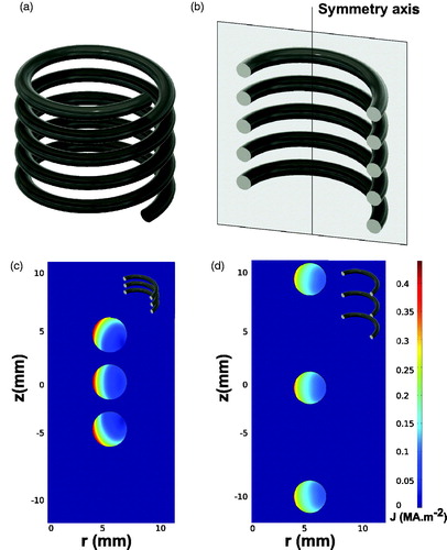
The electromagnetic interaction between nearby conductors prompts one additional constraint to the current flowing through them that is usually called proximity effect. This phenomenon can be particularly significant within closely wound wires, such as those of the inductor coil used in this case. Figure 1 illustrates the proximity effect by comparing two identical three-turn coils with 5 mm and 10 mm turn pitch. As can be seen in the Figure 1(c and d) the current density is highly constrained to smaller regions when turns of the coil are closer to each other.

Figure 1. (a) Solenoid coil (b) Sliced plane of the solenoid coil. Spatial distribution of the current density in the cross section of three turn solenoid with: (c) 5 mm turn pitch and (d) 10 mm turn pitch calculated by Finite Element Method (FEM) when 1 A intensity and 10 kHz frequency circulates across the coil.

In brief, it should be noted that the main limitation of using solid copper pipes lies in the effective resistance of the coil: increasing the frequency above certain limits decreases quite fast the efficiency and therefore the maximum achievable AC field amplitude. In our design, main dimensions of the coil have been fixed by starting from the more basic constraints, that are listed below in order of priority:

1. The sample holder size, which is a small polycarbonate cylindrical container of 100 µl of capacity, 11 mm long and 4.9 mm wide.

2. The pick-up coils that surround the sample, which should allow the air or N₂ to flow across the sample space.

3. The inner diameter and length of the coil were fixed to 12 mm and 41 mm respectively, in order to meet our homogeneity requirement (less than 3.5% over the pick-up coils length).

4. The number of turns that maximize the efficiency E_f has been obtained by Finite Element simulations.

Figure 2(a) shows the energy efficiency of the coil vs number of turns for the coil’s geometry mentioned above. In the case of the coil of one winding layer, the curve shows a maximum at N = 12 in 1 MHz. This maximum is related with the non-linear increase of the R due to the proximity effect (see Figure 2(b)) and it is slightly dependent on frequency (see Supporting Information Figure S6).

Figure 2. (a) Energy efficiency as a function of different number of turns calculated by FEM for 1, 2 and 3 winding layers coil. The simulations were performed supplying the coil with a 1 kW power amplifier and an AC current of 1 MHz frequency. (b) Equivalent resistance of the coil as function of number of turns for 1, 2, and 3 winding layers.

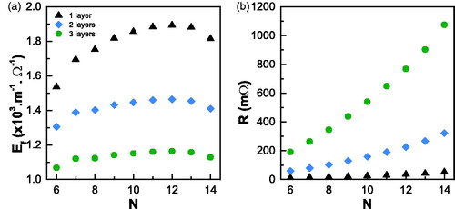
In coils with multiple winding layer the proximity effects (this time occurring also between conductors of consecutive layers) also degrade the efficiency. As shown in Figure 2(a) the most efficient coil is the one with a single winding layer. The reason for this is that when stacking more windings, equivalent series resistance increases faster than $\mathrm{\Pi }\left(\overrightarrow{r}\right)$ (Equation (4)(4) $$E_f=\mathrm{ }\sqrt{\frac{2{\mathrm{\Pi }}^2}{R}}$$(4) ) and thus the efficiency decreases.

As a result, the solenoid coil that maximizes the energy efficiency in the whole working frequency range should have one layer and 12 turn in 41 mm of total length.

2.2. Temperature system

To change the temperature of the sample during the measurement, a temperature controller was added to the setup.

The air flow is introduced (Figure 3(a)) inside the nylon cylinder located within the main coil. The temperature of the sample is measured with a non-resistible fiber optic thermometer (OpSens), placed near the sample and inside the nylon cylinder in contact with the airflow.

Figure 3. (a) Main coil cross section image showing the air flow system (b) Scheme of the air temperature controller.

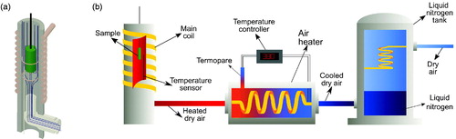
Figure 3(b) shows the scheme of the temperature system of the setup. The incoming air flow can be heated up to the desired temperature with an air heater resistance to change the temperature of the sample. When low temperatures are required, the pre-heating temperature of the system can be lowered simply by driving the incoming air flow through a winding copper coil immersed in Liquid Nitrogen, before reaching the heater. The temperature of the out coming air flow close to the heater output is under a feedback PID control with a standard thermocouple sensor. But in order to further keep the sample temperature as stable as possible a second feedback loop acts over the controller set point in response to changes of the fiber optic sensor located very close to the sample. Note that the sample always heats up during the AC application, so, isothermal conditions means in this case that the temperature of the air flow at the sample location must be kept constant during the experiment and the flow has to be high enough to remove the extra heat induced by the AC field in the sample.

2.3. AC hysteresis loops measurements and SAR calculations

The dynamic magnetization of the sample, M (t), (the projection of the total magnetization vector along the external AC field) is measured by a pick-up coil sensor. In this one, the time varying magnetization function M (t) is converted to a voltage signal according to Faraday’s law of induction.

The voltage coming from a single pick-up coil includes a background signal u^E, produced by the time-varying excitation magnetic field, which is always much larger (several orders of magnitude larger) than the signal induced by the MNPs sample itself (u^S). Therefore, the subtraction of the MNPs magnetization signal from the excitation one is very difficult to perform. Nevertheless, this redundant excitation u^E signal can be removed by winding two identical coils connected in series but oppositely wounded [20,21,34,35,43–45]. With this configuration, ideally, there is no u^E excitation signal when a homogeneous magnetic field is applied, which allows the subtraction of the MNPs sample signal (u^S). However, that cancelation of the excitation signal cannot be perfect because of the existing small phase shift between coils. This is due to capacity coupling effects between the pick-up coils and the main coil. Anyway, a very careful vertical positioning of the pick-up coil set allows attenuating the excitation contribution up to −65 dB at 134 kHz.

In order to eliminate the remaining interference excitation signal, the following procedure is proposed:

1. Measurement of the signal induced in the absence of sample (u^empty)

2. Measurement of the signal induced when the sample is in placed (u^tot)

3. Extraction of the MNPs signal by vector subtraction of empty signal: u^sample = u^tot −u^empty

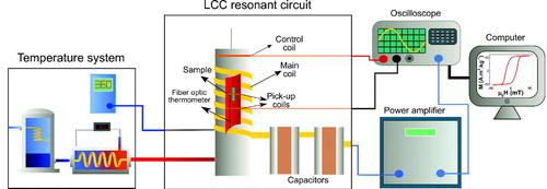
The AC hysteresis loops are obtained by plotting the dynamic magnetization, M (t), as a function of the magnetic field, µ₀H, measured by the pick up and control coils (see Main coil field calibration and Magnetization calibration sections in the Supporting Information), respectively. Both signals are acquired by an oscilloscope and then numerically integrated (Figure 4). Moreover, the coaxial cable influence has been taken into account and evaluated as is reported in the literature [21].

Figure 4. Complete scheme of the AC magnetometer set up.

The specific absorption rate (SAR) can be extracted by computing the area (A) enclosed by the loops, multiplied by the number of loops per second (frequency) and normalized by the sample concentration (mass per unit volume of the colloidal sample) [46]: (6) $$\mathit{SAR}\mathrm{ }\left(W{g}^{-1}\right)=\mathrm{ }\frac{f}{c}\mathrm{ }A=\frac{f}{c}\mathrm{ }{\mu }_0\mathrm{ }\oint M\mathrm{ }dH$$(6)

3. Results

3.1. Addressing the magnetic hyperthermia needs

In this section we show the powerfulness of the built high-field AC magnetometer in order to correctly characterize nanoparticle materials for hyperthermia. In this context, the adjective ‘high-field’ implies that the available field strength must be remarkably higher than the maximum amplitude achievable in previous AC magnetometers described in the literature [20,21,34,47]. They all work at most in the vicinity of 45 mT at one hundred kHz of excitation frequency. Exactly as it happens in standard DC magnetometry, the application of external magnetic fields, high enough to saturate the samples, is a fundamental premise to ensure a reliable analysis of their magnetic properties. In addition, if one has also the chance to perform isothermal measurements at different ambient temperatures, even below the freezing point of colloidal samples, one could be able to shed light on some of the issues that rise in hyperthermia experiments:

1. Magnetic saturation conditions in hyperthermia experiments. The relation between the magnetically saturated AC hysteresis loops and the saturation of the SAR.

2. The influence of excitation frequency, particle size and shape on the area of the hysteresis loops.

3. The contribution of mechanical rotation of particles and particle assemblies to experimental SAR in viscous media.

4. The optimal magnetic field excitation parameters (intensity and frequency) for hyperthermia experiments.

5. The heat transfer from the heat source (MNPs) to the medium.

Aiming to address some of the previous issues, we need a touchstone, a suitable series of samples acting as a test case where experimental trends can be easily compared with available models, such as those based on the Linear Response Theory (LRT) [48], the Stoner–Wohlfarth model based theories (SWMBTs) [49] (also referred as high energy barrier approximation [50] or two levels approximation) or the Stochastic Laudau-Lifshitz-Gilbert equation (LLG) [51].

3.2. Characterization of samples

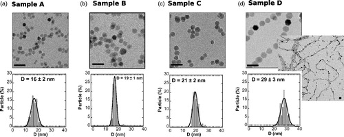
We have prepared four different samples of magnetite (Fe₃O₄) nanoparticles with sizes ranging from 16 nm to 29 nm following a recently published method with few modifications [30]. This range of particle size (16–29 nm) is usually considered as a good choice to maximize the SAR. These MNPs present a cuboctahedral shape and a narrow size distribution of roughly gaussian shape, as it can be observed in the TEM images and in their corresponding histograms of Figure 5. In addition, X-ray diffraction on powder samples (see Supporting Information Table T2) indicates that the samples are single crystals. As shown in Figure 5, clustering effects are not severe in the studied samples. However, it can be observed how the largest particles (sample D) show a clear chaining tendency (Figure 5(d)).

Figure 5. TEM images of samples (a) A, (b) B, (c) C and (d) D together with their corresponding size distributions. Scale bar 50 nm.

Figure 6 shows DC magnetometry measurements of samples A-D performed in diluted samples, prepared by depositing a drop of the colloidal dispersion on a laboratory blotting paper to prevent fast diffusion and agglomeration of colloidal particles. Additionally, saturation magnetization values have been obtained by measuring dried powder samples up to high DC field in a standard SQUID magnetometer. The total magnetic moment can be correctly normalized by subtracting the organic contribution to the total mass, which is determined by a Thermogravimetric Analyzer (TGA). The more significant conclusions are listed below:

Figure 6. First row: DC hysteresis loops at 5 K (red line) and 300 K (black line) for samples (A) A, (b) B, (c) C and (d) D. Second row: ZFC-FC curves (black line) together with derivatives of ZFC magnetization (blue line) for samples (e) A, (f) B, (g) C and (h) D.

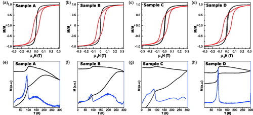
• It shows that the magnetic phase of the nanoparticles is magnetite. The ZFC-FC curves of Figures 6(e–h) present a sudden drop of the magnetization when crossing 80–100 K temperature range. This drop corresponds to the Verwey trasition, the clear hallmark of magnetite. Magnetic phase is ‘roughly’ magnetite. We say ‘roughly’ because the precise stoichiometry of the crystalline phase can differ from that of pure magnetite [30,52].

• The low temperature hysteresis loops shown in Figure 6(a–d) (red line), where thermal fluctuations are damped down, are characteristic of uniaxial single domains oriented at random, with remanence approaching 0.5 and coercive field values (µ₀H) ranging from 40 to 50 mT. This is readily apparent by comparing experimental data with SWMBTs simulations, as can be seen in the Supporting Information Figure S12. Note that the good matching to SWMBTs behavior does not necessary mean that our MNPs are magnetically isolated. At least, we are certain that particles are not forming large and chaotic clusters where dipolar interactions would favor antiparallel configuration of particles’ magnetization and then a remarkably decrease of the reduced remanence.

• Thermal fluctuation effects become strongly significant at room temperature (Figure 6(a–d) (black line)), to the point of almost removing the hysteresis (remanence and coercivity) in three of the samples with sizes of 16, 19 and 21 nm. The three smallest show clear blocking effect below room temperature and the largest, 29 nm, is the only one where thermal effects are small (see Figure S9 of the Supporting information).

• The single domain magnetization values obtained from high field DC measurements (up to 2 T, see Supporting Information S11) range from 80 to 89 Am²kg⁻¹. These are rather approximate to that of the pure magnetite (92 Am²kg⁻¹), confirming the high purity of the crystalline phase. In any case, magnetization variations from sample to sample are not very significant so we take an average of 86 Am²kg⁻¹ (or conversely 450 kAm⁻¹) for the hysteresis loops simulations that will be discussed later.

Therefore, we can conclude that the selected samples are magnetite phase single crystals showing weak interparticle interactions.

3.3. AC hysteresis loops at room temperature

The measurements shown in this section correspond to hysteresis loops recorded at different frequencies between 134 and 835 kHz. They can be easily used to calculate the SAR through Equation (6)(6) $$\mathit{SAR}\mathrm{ }\left(W{g}^{-1}\right)=\mathrm{ }\frac{f}{c}\mathrm{ }A=\frac{f}{c}\mathrm{ }{\mu }_0\mathrm{ }\oint M\mathrm{ }dH$$(6) .

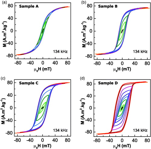
First of all, we present measurements performed at 134 kHz because at this frequency, the maximum achievable AC field becomes as high as 90 mT. As observed in Figure 7(a–d) the magnetization of all the samples saturates at fields higher than 50 mT and hysteresis area remarkably grows with the particles’ size. It is noteworthy that the loop of the largest sample, with permanent magnetized particles, has a highly square shape, with a large remanence close to 80 Am²kg⁻¹.

Figure 7. AC hysteresis loop of sample (a) A, (b) B, (c) C and (d) D taking at room temperature (RT) under magnetic field of 90 mT at 134 kHz. Note that all the samples saturate almost at 50 mT. As size of the sample increase, the loops broaden obtaining a square shape loop in the sample D.

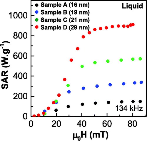
Figure 8 shows the experimental SAR curves built after computing the hysteresis loop area as function of the external field amplitude in liquid state. It is to note that, in the samples with largest particles’ size (samples C and D), the hysteresis area and SAR increases with field in a strongly non-linear fashion, saturating with field amplitudes above the threshold of 50 mT. The slope changes of SAR versus μ₀H curve presented in Figure 8 are less pronounced in the smallest particles (samples A and B).

Figure 8. SAR versus field intensity curves obtained from the area of AC hysteresis loops under the field frequency of 134 kHz at liquid state. Measurements are performed at room temperature in liquid state for four samples.

3.4. AC hysteresis loops in frozen solutions

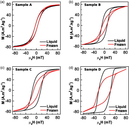
Obviously, given that samples are aqueous solutions, the colloidal magnetic particles are able to mechanically rotate during the experiments. It happens due to different mechanical effects that potentially exist in a liquid medium: (1) the rotational Brownian motion of small colloidal particles, (2) the mechanical rotation of magnetic particles toward the magnetic field direction due to the magnetic torque and (3) the potential spatial rearrangement of particles in chains, either preexisting in the colloidal sample due to dipolar interactions or induced by the applied AC magnetic field during measurements. In order to avoid the potentially complex problem of understanding a mix of different physical mechanisms happening at the same time and to discriminate the effect of physical rotation, AC loops can be directly measured below the freezing point of the solvent, water in this case. Figure 9 shows the AC hysteresis loops at 253 K (–20° C), corresponding to maximum field at 134 kHz, in the four studied samples after freezing them. These hysteresis loops (red lines) are compared with those obtained in liquid samples (black lines).

Figure 9. AC hysteresis loops of sample (a) A, (b) B, (c) C and (d) D under magnetic field of 90 mT and frequency of 134 kHz in room temperature/liquid state (black) and frozen state (red).

In these experiments the temperature of the air flowing through the sample chamber is kept constant at 253 K, low enough to freeze the water solvent completely. Figure 10 shows the experimental SAR curves built after computing the hysteresis loop area as function of the external field amplitude in frozen state. Figure 10 also shows the corresponding simulations performed using SWMBTs [49], that will be analyzed in the discussion section.

Figure 10. SAR versus field intensity curves obtained from the area of AC hysteresis loops under the field frequency of 134 kHz at frozen state. The dots indicate the experimental results and the lines their corresponding simulations using Stoner–Wohlfarth model based theories (SWMBTs).

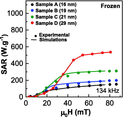
Remarkable differences between liquid and frozen samples are very visible in Figure 9. Sample D (largest particles) shows much less hysteresis area in the frozen state. This is basically due to the much smaller value of the remanence magnetization, while the coercive field remains almost unchanged. Note also that the anisotropy field (the field required for saturation) is close to the maximum of the available span of the AC magnetometer at 134 kHz (90 mT). In consequence, maximum SAR of sample D in the frozen state is reduced by a factor of 0.6 relative to the liquid case (540 W/g vs 910 W/g, red curves in Figures 8 and 10). On the contrary, hysteresis loops of sample A remains approximately unchanged after freezing (Figure 9(a)), while samples B and C stands on the midway between the behavior of samples A and D (Figure 9(b,c)). Consequently, the SAR of the sample A is unchanged whereas it is reduced by a factor of 0.52 and 0.58 in Samples B and C, respectively.

Figure 11 presents the dependence of the AC hysteresis loops and their area with frequency (see Equation (6)(6) $$\mathit{SAR}\mathrm{ }\left(W{g}^{-1}\right)=\mathrm{ }\frac{f}{c}\mathrm{ }A=\frac{f}{c}\mathrm{ }{\mu }_0\mathrm{ }\oint M\mathrm{ }dH$$(6) ). Figure 11(e–h) shows the experimental values of SAR/f versus magnetic field intensity at 134 kHz, 561 kHz and 835 kHz frequencies (dots) and their corresponding simulations using SWMBTs (lines) in frozen media. The hysteresis area increases with frequency for particles in frozen solution (dots), but this increment depends critically on particle’s size. Thus, for instance, the increase of SAR/f with frequency is particularly intense in the case of sample A, composed of particles of 16 nm (Figure 11(e)). As particle’s size increases, SAR/f curves tend to be closer (Figure 11(f–g)). Finally, SAR/f curves in sample D almost collapse in a single one (Figure 11 (h)). This behavior can also be observed in Figure 11(a–d), where AC hysteresis loops of the four samples are plotted at different frequencies under 30 mT magnetic field intensity. Note that in sample A (Figure 11(a)), as frequency increases the hysteresis loops get widened. This hysteresis growth is less pronounced in sample B and C (Figure 11(b–c)). Finally, in sample D (Figure 11(d)), the hysteresis loops of different frequencies are almost superimposed in a single curve.

Figure 11. First row: AC hysteresis loop of sample (a) A, (b) B, (c) C and (d) D at 134 kHz (red), 561 kHz (green), 835 kHz (blue) and DC (black) in frozen media at 30 mT. Second row: SAR/f versus field intensity curve obtained from the area of AC hysteresis loops at 134 kHz (red), 561 kHz (green) and 835 kHz (blue) of sample (e) A, (f) B, (g) C and (h) D. The dots indicate measurements performed in frozen solutions and lines their corresponding simulations by using SWMBTs [49].

4. Discussion

The main purpose of this work is not aimed neither to present new theoretical models nor to discuss the magnetic properties of new samples. Rather, we intend to understand previous results in the light of the existing models, which have proved useful to explain and predict to a great extent the magnetic properties pertaining to hyperthermia. We will focus on those properties for which our novel AC magnetometer provides new experimental data that has not been available, so far. Our aim is to answer some of the issues previously raised at the beginning of the experimental section.

4.1. The question of the mechanical rotation contribution to hyperthermia

When magnetic particles immersed in a liquid medium are considered as free-rotating isolated objects, whose magnetization is supposed to be pinned to an easy magnetization axis, their dynamical response to AC magnetic fields can be calculated in the framework of magnetic single domains theories [53–55]. In brief, the available predictions suggest that at small enough field amplitudes, meaning that they are much smaller than the anisotropy field ($H_k=\frac{2K_{\mathit{eff}}}{{\mu }_0{M}_s}$) for single domains with uniaxial anisotropy, the external torque exerted by the alternating magnetic field should produce forced angular oscillations of the particles at the excitation frequency of the field [53]. The amplitude and phase of this vibration will depend on applied magnetic field frequency and will peak (they are in resonance) when excitation frequency approaches the Brownian relaxation time [56]. This relaxation time can be determined from the particlés size (hydrodynamic volume V_h), the viscosity of the medium η, and the external AC magnetic amplitude H_AC, by the following expression [56]: ( 7) $$2\mathrm{ }\pi {\tau }_{B-\mathit{eff}}\left(H_{AC}\right)=\mathrm{ }{\tau }_B\mathrm{ }{\left[1+{\mathrm{ }\left(\frac{\mu {\mu }_0{H}_{AC}}{k_{B}T}\right)}^2\right]}^{-0.5}\mathrm{ }$$( 7) where ${\tau }_B$ is the well-known Brownian relaxation time at zero field, $\frac{3\eta {V_h}^3}{k_{B}T},$ $k_B$ is the Boltzmann constant and µ is the relative magnetic permeability. According to this model, pseudo-spherical particles of magnetite (M_s = 480 kA.m⁻¹) in the size range 16–20 nm are expected to turn around at a rate of the order of hundreds of kHz, just in the range of the AC excitation frequency used in hyperthermia. Note that, if thermal energy is much higher than the anisotropy energy, the particle magnetic moment ‘unpins’ from the easy axis and therefore becomes mostly collinear with the external AC field at all times. Thus, the magnetic torque and Brownian effect tend to be removed.

However, the strength of AC fields of interest to hyperthermia is far from being small relative to the anisotropy field, particularly for magnetite particles. Assuming that the anisotropy field of a typical magnetite particle lies around ∼ 40 kA/m (or ∼ 50 mT), hyperthermia AC fields easily approach or overcome the anisotropy energy barrier for magnetization reversal (K_eff v).

In general, Neel relaxation time as a function of the external field can be estimated from the following equation [56]:

(8) $${\tau }_N{\left(H_{AC}\right)}^{-1}=\mathrm{ }{\tau }_0^{-1}\left(1-h^2\right)\text{ × }\left\{\left(1+h\right)\exp \left[\left(\frac{-k_{\mathit{eff}}v}{k_{B}T}\right)\mathrm{ }{\left(1+h\right)}^2\right]+\mathrm{ }\left(1-\mathrm{ }h\right)\exp \left[\left(\frac{-k_{\mathit{eff}}v}{k_{B}T}\right)\mathrm{ }{\left(1-\mathrm{ }h\right)}^2\right]\mathrm{ }\right\}\mathrm{ }$$(8) where $h=\frac{H}{H_k}$ and τ₀ is a constant (10⁻⁹–10⁻¹⁰ s). In these conditions, Neel relaxation can be strongly accelerated by several orders of magnitude depending on the field strength [56], leading Brownian rotations to be accordingly suppressed.

The results of Figure 9(a) indicate that in sample A, thermal fluctuations alone remove the Brownian rotation contribution to the SAR: hysteresis loops obtained at any AC amplitude remain almost unchanged upon the freezing of water. If the anisotropy constant is in the range of 10–15 kJm⁻³ [46,52], Neel relaxation time is always smaller than ∼10⁻⁸–10⁻⁹ s and therefore always much faster than Brownian relaxation time calculated from Equation (8)(8) $${\tau }_N{\left(H_{AC}\right)}^{-1}=\mathrm{ }{\tau }_0^{-1}\left(1-h^2\right)\text{ × }\left\{\left(1+h\right)\exp \left[\left(\frac{-k_{\mathit{eff}}v}{k_{B}T}\right)\mathrm{ }{\left(1+h\right)}^2\right]+\mathrm{ }\left(1-\mathrm{ }h\right)\exp \left[\left(\frac{-k_{\mathit{eff}}v}{k_{B}T}\right)\mathrm{ }{\left(1-\mathrm{ }h\right)}^2\right]\mathrm{ }\right\}\mathrm{ }$$(8) .

In this case reversal mechanism largely dominates over the rotation ones. For samples B, C and D, composed of larger particles, Brownian relaxation becomes faster than Neel relaxation at zero field, particularly for sample D (29 nm), assuming that particles of the assembly do not form clusters and the hydrodynamic volume is similar to particle’s volume. Given that Neel relaxation will be much faster at high enough field amplitudes, the changeover between rotation and reversal mechanisms could lead to a complex behavior of the hysteresis area as a function of the AC amplitude in samples B, C and D, as predicted from the available calculations in the literature [53].

On the other hand, particles with permanent magnetization tend to agglomerate easily in pseudo spherical clusters and/or to form chains. The size of these large objects makes them unable to respond to the magnetic field excitation in the form of vibrations. However, when magnetization moment vector of a magnetic object (a single particle or a whole chain for instance) irreversibly switches between different orientations driven by the applied magnetic field, the time averaged magnetic torque over such object is non-zero. As a result, the magnetization easy axis is impelled to rotate toward the magnetic field lines after a given number of field cycles. This alignment effect has been predicted from direct numerical calculations of the dynamical equations for single magnetic domains [53], but it can be also qualitatively understood appealing to simpler arguments. For instance, let’s assume that the instantaneous net magnetic moment vector m(t) takes the following simple form as a function of time in response to an external AC magnetic field given by $\mathit{H}=H_0\text{sin}\left(\mathit{\omega }t\right){\mathrm{ }\mathit{u}}_{\mathit{H}}$ (9) $$\mathit{m}=\mathrm{ }{m}_{0\mathrm{ }}\text{sin}\left(\mathit{\omega }t-\phi \right){\mathrm{ }\mathit{u}}_{\mathit{H}}+m_{0\mathrm{ }}\text{cos}\mathrm{ }\left(\mathit{\omega }t-\phi \right){\mathit{u}}_{\perp }$$(9) where ${\mathit{u}}_{\perp }\mathrm{ }$ is the unit vector perpendicular to${\mathrm{ }\mathit{u}}_{\mathit{H}}.$ Even though, Equation 9(9) $$\mathit{m}=\mathrm{ }{m}_{0\mathrm{ }}\text{sin}\left(\mathit{\omega }t-\phi \right){\mathrm{ }\mathit{u}}_{\mathit{H}}+m_{0\mathrm{ }}\text{cos}\mathrm{ }\left(\mathit{\omega }t-\phi \right){\mathit{u}}_{\perp }$$(9) cannot represent a correct solution of the dynamical problem, it works here as a crude approximation that can represent the first harmonic of the magnetic moment components, parallel and perpendicular to the magnetic field direction (µH). Assuming that the easy axis of the magnetic object does not have time to appreciably rotate during a complete cycle of the external field, this torque can be averaged in a field cycle as: (10) $${〈T〉}_{\mathit{cycle}}=\mathrm{ }\frac{\mathit{\omega }}{2\pi }\mathrm{ }{\int }_0^{\mathrm{2n/}\mathit{\omega }}{\mu }_{0\mathrm{ }}{m}_{0\mathrm{ }}{H}_0\text{sin}\left(\mathit{\omega }t\right)\text{cos}\left(\mathit{\omega }t-\phi \right)dt=\mathrm{ }\frac{1}{2}\mathrm{ }{\mu }_0{m}_0{H}_0\text{sin}\phi$$(10)

In consequence, this effective mechanical torque is acting always, provided that the magnetic moment component perpendicular to the magnetic field is non-zero. Note that when particles become randomly agglomerated the net magnetic moment of the whole cluster m₀ tend to be close to zero at the remanence state of the system (H = 0) and collinear with H at some other instant so the net magnetic torque becomes negligible.

Naturally, thermal or stochastic fluctuation of the object in the liquid works to remove the orientation effect, so, large net and permanent magnetic moments are essential to produce a full alignment of the magnetic object with the field. In such case, the reduced remanence magnetization becomes much higher than 0.5 for almost any AC field amplitude. The mechanical orientation along the field lines can be observed very clearly in sample D, and in a weaker way in samples B and C, composed of particles of smaller size. It is obvious that this mechanism is size-sensitive, and also happens with isolated or non-interacting particles. However, this effect has been reported as particularly intense in magnetotactic bacteria [27,57], where the chain arrangement of magnetosomes strongly favors the orientation of bacteria in water-based solutions. Similar behaviors have been observed in free Fe MNPs at 25 mT [58] and FeC MNPs at 44 mT (both at 93 kHz) [29]. It is worthy to note that particles of samples B, C and D have a trend toward chaining with the aim to reduce the magneto-static energy (as shown in Figure 5(d)). These chains can carry a large permanent magnetic moment. Particularly in sample D, this tendency is stronger and the large squareness of the AC loops (for any field amplitude) could suggest the formation of large chains with well-defined easy axis that become mostly aligned in the magnetic field lines during AC magnetometry experiments. However, the rotation of each individual particle toward the field lines can also contribute to this mechanism and must be considered as a possible explanation.

In any case the opportunity of fast ‘removing’ any possible mechanical motion in-situ is interesting for hyperthermia characterization because magnetic objects are not expected to be freely rotating when they are attached to biological entities and quantitative models are aimed at immobilized particles [31].

4.2. The Specific Absorption Rate and the size effect

The size of particles really matters to maximize SAR if the AC excitation available is limited by technical or biomedical considerations [25,30]. This question has been largely discussed in the literature. In brief, Linear Response Theory (LRT) clearly predicts that optimal size for particles of magnetite is situated around 18–20 nm [59]. We explicitly say magnetite because this optimal size depends ultimately on the anisotropy energy of the particle: it would be greatly different in cobalt containing ferrites or in Fe metallic alloys, for instance. But LRT only applies to small AC amplitudes so, the existence or absence of a well-defined peak in the curves of SAR versus size of particles becomes a tricky question. The best answer is, that it depends on the excitation (frequency and field), and our results presented in Figure 12 confirm this point.

Figure 12. SAR/f versus particles’ size curves at (a) 22 mT (b) 28 mT and (c) 45 mT magnetic field intensities and 134 kHz (black line), 561 kHz (blue line) and 835 kHz (green line) frequencies.

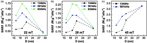
Figure 12 shows the curve of SAR/f as a function of particle’s diameter at 22 mT, 28 mT and 45 mT magnetic field intensities. Figure 12(a,b) present a maximum at 21 nm at 134 kHz frequency that shifts down to 19 nm at higher frequencies (561 and 835 kHz). In addition hysteresis area (and SAR) of samples A and B increases very significantly with frequency (Figure 11(e–f)). This frequency driven effect reflects, in fact, the dependence of the coercive field on frequency, particularly intense for the smaller single domain volumes, as explained in the literature (see Usov et al. [60], Carrey et al. [49] or the Supporting Information Figure S14).

For higher field values (see Figure 12(c)), it is noteworthy that SAR/f clearly increases with particles’ size (in the studied range), which is also evident by quick inspection of the major loops of each sample. As discussed below, this behavior has been successfully predicted by several authors [61,62], using different models. Suffice it to say, that our results confirm the predictions of these models.

4.3. The Specific Absorption Rate as a function of field and frequency

We do not pretend an accurate description of individual samples but only to outline the most significant qualitative trends, which are common to all of them and are noticeable only by using our experimental set-up.

Stoner-Wohlfart model based theories (SWMBTs) for magnetic single domains predict two properties related to the magnetic hysteresis that are readily identifiable in our experimental measurements: (1) a very steep increase of the hysteresis area at around certain threshold field amplitude followed by a saturation field amplitude at which the hysteresis (or SAR) does not increase any longer and (2) these maximum hysteresis area and SAR increase with particle size [30,49]. In these models, magnetization is considered as a single vector (magnetic moment per unit volume) anchored to the instantaneous energy minima states. This approach is valid provided that the magnetic anisotropy energy of the particle is much larger than the thermal energy (k_BT) (high energy barrier approximation). Otherwise, thermal fluctuations should be incorporated in the model and one has to deal with the stochastic version of the LLG equation and find the probability distribution function for magnetization as a function of time [50]. In any case, the complete lack of full experimental evidence about these questions was still hindering the validation of these or any other models.

The results presented in Figures 7, 8, 9 and 10 imply, to a large extent, the experimental confirmation of the most significant theoretical predictions. The most eye-catching agreement between experiments and theory (Figure 10) arises immediately: the four experimental SAR versus field intensity curves tend to saturate at some values that scale very well with the simulations obtained from the SWMBTs model applied to particles of different size. With the aim of building a more realistic and predictive model for our particular samples, we have considered a normal distribution of uniaxial anisotropy constants (see Effective anisotropy constant distribution section in the Supporting Information for further details). At this point we are implicitly assuming that this uniaxial ‘effective’ anisotropy is the result of combining the magnetocrystalline and the shape effects as well as any hypothetical contribution from dipolar interactions, particularly intense in chains [57,63]. Note that TEM images show particles with different degree of elongations and forming chains of different lengths and both effects should favor the onset of a wide range of effective anisotropies. Best fits are obtained by averaging a normal distribution of anisotropy constants with a standard deviation of 5 kJm⁻³ and centered at: Sample A 16 kJm⁻³, Sample B, 16 kJm⁻³, Sample C, 15 kJm⁻³ and Sample D, 19 kJm⁻³. It should be noted that size distribution is not implicitly considered for the simulations, so this standard deviation value (5 kJm⁻³) should also reflect the particlés size dispersion. For simplicity, the magnetization (450 kAm⁻¹) has been kept equal for all of them, and other details of the model are given in the Supporting Information. On the other hand, these values for the effective anisotropy constants would be valid at 253 K (temperature of the frozen samples). If one assumes that shape anisotropy contribution is dominant, these effective magnetic anisotropies will depend on temperature as ∝ M ², being M the particle’s magnetization. Since the magnetization decrease between 253 and 290 K is near 2% (see Supporting Information S10), effective anisotropy constant would experience a 4% reduction from 253 K to 290 K, which is not significant because is within tolerance of the theoretical approach. It should be noted that, such form of thermal dependence (as M ²) cannot be extrapolated to lower temperatures in our case, due to the presence of the Verwey phase transition at around 100 K. A detailed analysis of this issue requires the collection of additional data as a function of temperature and a more complex modeling to take account for the thermal dependence of the magnetocrystalline contribution to the anisotropy that is out of the scope of this work. This type of study have been already done in the literature, either with magnetosome [64], whose thermal behavior is expected to be similar to the samples presented in this work, or very recently with Mn-Zn ferrites [65].

The overall agreement between experiments and simulations in both SAR evolution (Figure 10) as well as in AC hysteresis loops (see Supporting Information Figure S13) is quite surprising since simplifications made in the modeling are really strong: size distribution has been not taken into account and, most importantly, magnetic dipolar interactions have not been explicitly considered. Obviously, given that the sample D is composed of relatively large particles of 29 nm and seems to be linked in chains, with minor influence from thermal effects, the SAR versus field curve displays a sharper saturation effect and, in overall, a better matching with the SWMBTs model. Even the samples composed of significantly smaller particles (A and B) follow the qualitative trends predicted by SWMBTs (Figure 10). These findings have two important implications:

• The heating power of magnetic MNPs, calculated by AC magnetometry, is a ‘safe’ starting point for modeling the thermal transfer from MNPs to different surrounding media, which is the ultimate goal of magnetic hyperthermia experiments. Therefore, AC magnetometry and calorimetry become very complementary techniques: the former can be used to know the input heat power the latter detects the transfer rate of this power to the environment as the final outcome of the magnetic actuation.

• In ‘small’ particles the effective anisotropy constant K_eff can be obtained from the blocking temperature measurement, but for larger particles this temperature can be unattainable. In the latter case, the determination of area vs AC intensity curve up to high field intensities becomes a powerful way to roughly estimate K_eff, for instance, throught the derivative of the curve. For isolated particles, this estimation can also be done either by directly ‘matching’ the SAR versus field intensity experimental curve to a model for dynamical loops, or by using some analytical formula, as proposed in the literature [49]. Note that, in general, the effective anisotropy constant, as estimated from SAR versus AC field curve, will include the contribution from dipolar interactions, particularly when MNPs are arranged in chains.

Also the influence of the excitation frequency can be qualitatively understood within the same framework provided by the SWMBTs because the simulations reproduce reasonably well the experiments (Figure 11). Simulations performed at different frequencies predict the marked contrast between the dispersion obtained in sample A (Figure 11(e)), where curves of SAR/f(H) at different frequencies strongly diverge and sample D, where these curves are mostly frequency independent (Figure 11(h)).

4.4. Optimizing the excitation conditions for practical treatment as a function of size

Eddy current effects in extended ‘conducting’ bodies produce a nonspecific heating that can affect negatively healthy tissues of potential human patients. The strength of these eddy currents depends on the product of Hf, so different safety limits for the maximum acceptable (Hf) have been proposed. For the so-called Atkinson-Brezovich criterion [66,67], (Hf) is fixed to 4.85 × 10⁸ Am⁻¹s⁻¹ while for the weaker approach of Hergt [10] the limit is ten times larger, Hf ∼ 5 ×10⁹ Am⁻¹s⁻¹. In any case, no matter what particular limit is taken, its very existence itself imposes an optimal combination of magnetic excitation variables, magnetic field amplitude and frequency, for each sample that can be deduced from the dependence on field amplitude of the SAR normalized by the frequency, SAR/f (Figure 11(e–h)). Considering, for instance, the Hergt criterion, given a field amplitude (H), the maximum acceptable frequency is determined by: f_limit (H) = 5 × 10⁹Am⁻¹s⁻¹/H, so the maximum achievable SAR (named as SAR_limit) can be calculated as: (11) $${\mathit{SAR}}_{\mathit{limit}}\left(H\right)={\left(\frac{\mathit{SAR}}{f}\right)}_{f_{\mathit{limit},H}}\mathrm{ }.\mathrm{ }{\mathrm{ }f}_{\mathit{limit}\mathrm{ }}\left(H\right)=\mathrm{ }{\left(\frac{\mathit{SAR}}{f}\right)}_{f_{\mathit{limit},H}}.\mathrm{ }5\text{\hspace{0.17em}x\hspace{0.17em}}\frac{{10}^9}{H}$$(11)

Note that SAR/f will be, in general, a function of the frequency as well as the field, so it must be calculated for f = f_limit, except in those cases where curves SAR/f (H) collapse in a single universal curve, as in sample D. Since the experimental data and/or the corresponding modeling points are only available for three discrete frequencies, SAR_limit(H) has been obtained by interpolation of the existing SAR/f curves, for sample A, B and C.

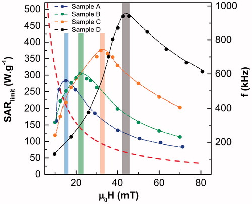
Figure 13 shows the SAR_limit(H) curve calculated from Equation (11)(11) $${\mathit{SAR}}_{\mathit{limit}}\left(H\right)={\left(\frac{\mathit{SAR}}{f}\right)}_{f_{\mathit{limit},H}}\mathrm{ }.\mathrm{ }{\mathrm{ }f}_{\mathit{limit}\mathrm{ }}\left(H\right)=\mathrm{ }{\left(\frac{\mathit{SAR}}{f}\right)}_{f_{\mathit{limit},H}}.\mathrm{ }5\text{\hspace{0.17em}x\hspace{0.17em}}\frac{{10}^9}{H}$$(11) for the four samples, A-D. In this figure, the red dash curve is the hyperbolic function f_limit(H) = 5 × 10⁹/H and serves up to determine which frequency corresponds to a given SAR_limit.

Figure 13. Maximum achievable SAR, SAR_limit, under the Hergt criterion for all the samples. The red dashed curve is the acceptable maximum frequency, f_limit(H) = 5 × 10⁹Am⁻¹s⁻¹/H, for a given magnetic field intensity following the Hergt criterion. The optimal excitation intensity to get the maximum SAR_limit value is indicated with colored bars (each color corresponds to one of the samples). The intersection of the red dashed curve and the colored bar of each sample shows the optimal frequency for obtaining the maximum SAR_limit value.

The following features can be highlighted:

• All curves peak at some optimal magnetic field amplitude whose values are increasing with the particle’s size. Obviously, the corresponding working frequencies under the safety limit of Hergt are decreasing accordingly.

• Maxima of the curves SAR_limit(H) are increasing with size, in such a way that larger particles can potentially produce more heat by choosing the appropriate excitation conditions. The maxima and the corresponding excitation parameters found are: Sample A, 285 Wg⁻¹ at (15 mT and 417 kHz), Sample B, 305 Wg⁻¹ at (22 mT and 284 kHz), Sample C, 375 Wg⁻¹ at (32 mT and 195 kHz) and Sample D, 480 Wg⁻¹ at (45 mT and 139 kHz).

Of course, previous features hold for a series of particles with similar composition and morphology. Finally, it is worthy to mention that determining these optimal conditions requires AC magnetometers as versatile as possible, meaning that the available field span and working frequencies should be broad enough.

5. Conclusions

We have developed a versatile AC magnetometer able to work in a large range of frequencies (100 kHz − 1MHz) that are relevant for magnetic hyperthermia, and capable of applying remarkably higher field intensities that those existing so far. With a power amplifier limited to 1 kW, the geometry of the coil was carefully designed to reach 90 mT at 134 kHz and 30 mT at the maximum frequency of 950 KHz, in all cases with a high degree of homogeneity in a volume of approximately 100 mm³. It has been demonstrated than skin and proximity effects strongly constrain the optimal number of turns as well as the use of more winding layers. The best geometry for a coil of 12 mm in diameter and 41 mm in length corresponds to a single layer 12 turn coil.

It has been shown that the variable temperature system that makes use of air flow through the sample chamber is able to fix isothermal ambient conditions at the sample container. Thus, by freezing the sample solution, we have been able to decouple pure mechanical effects from the intrinsic relaxation of the magnetization across the lattice.

The results obtained in a test sample series of magnetite nanoparticles (16–29 nm) confirm that the hysteresis area (and conversely the SAR) saturate at moderate field intensities, above 50 mT.

It has also been confirmed that this saturation or maximum SAR depends strongly on particles’ size and on the angular distribution of easy magnetization axes. The overall dependence on field and frequency of SAR versus field amplitude curves fit rather accurately with the Stoner–Wohlfarth model based theories (SWMBTs) of uniaxial single magnetic domains. Finally, the optimal magnetic field intensity and frequency for maximizing the SAR within the safety limit have been calculated for each sample. This calculation is vital to choose the optimal samples for each magnetic treatment experiments in which excitation frequency is often fixed. To determine the optimal magnetic field parameters, a high field AC magnetometer that works in a wide frequency range, as the one developed in this work, is necessary.

Acknowledgments

I.R. acknowledges the Basque Government for her fellowship (PRE 2017 2 0089) and for the financial supporting of this work (IT-1005-16). The authors acknowledge the technical and human support provided by Javier Alonso Valdesueiro, Jorge Feuchtwanger and SGIker(UPV/EHU). Dr I. Castellanos-Rubio thanks the The Horizon 2020 Programme for the financial support provided through a Marie Sklodowska-Curie fellowship (798830).

Disclosure statement

No potential conflict of interest was reported by the author(s).

Additional information

Funding

This work was supported by the Basque Government under Grants PRE 2017 2 0089, IT-1005-16 and GU IT1226-19; Horizon 2020 under fellowship (798830).

References

- Jordan A, Wust P, Scholz R, et al. Magnetic Fluid Hyperthermia (MFH). In: U. Häfeli, W. Schütt, J. Teller, and M. Zborowski, editors, Scientific and clinical applications of magnetic carriers. Boston, MA: Springer US; 1997. pp. 569–595.
- Pankhurst QA, Connolly J, Jones SK, et al. Applications of magnetic nanoparticles in biomedicine. J Phys D: Appl Phys. 2003;36(13):R167–R181.
- Jordan A, Scholz R, Wust P, et al. Magnetic fluid hyperthermia (MFH): cancer treatment with AC magnetic field induced excitation of biocompatible superparamagnetic nanoparticles. J Magn Magn Mater. 1999;201:413–419.
- Mornet S, Vasseur S, Grasset F, et al. Magnetic nanoparticle design for medical diagnosis and therapy. J Mater Chem. 2004;14(14):2161–2175.
- Perigo EA, Hemery G, Sandre O, et al. Fundamentals and advances in magnetic hyperthermia. Appl Phys Rev. 2015;2(4):041302.
- Jordan A, Wust P, Fahling H, et al. Inductive heating of ferrimagnetic particles and magnetic fluids: physical evaluation of their potential for hyperthermia. 1993. Int J Hyperthermia. 2009;25(7):499–511.
- Ma M, Wu Y, Zhou J, et al. Size dependence of specific power absorption of Fe3O4 particles in AC magnetic field. J Magn Magn Mater. 2004;268(1–2):33–39.
- Lima E, Torres TE, Rossi LM, Rechenberg HR, et al. Size dependence of the magnetic relaxation and specific power absorption in iron oxide nanoparticles. J Nanopart Res. 2013;15(5):1654.
- Barrera G, Coisson M, Celegato F, et al. Cation distribution effect on static and dynamic magnetic properties of Co1-xZnxFe2O4 ferrite powders. J Magn Magn Mater. 2018;456:372–380.
- Hergt R, Dutz S, Muller R, et al. Magnetic particle hyperthermia:¨ nanoparticle magnetism and materials development for cancer therapy. J Phys: Condens Matter. 2006;18(38):S2919–S2934.
- Branquinho LC, Carrião MS, Costa AS, et al. Effect of magnetic dipolar interactions on nanoparticle heating efficiency: implications for cancer hyperthermia. Sci Rep. 2013;3:2887.
- Lee J-H, Jang J-t, Choi J-s, et al. Exchange-coupled magnetic nanoparticles for efficient heat induction. Nat Nanotechnol. 2011;6(7):418–422.
- Fortin J-P, Wilhelm C, Servais J, et al. Size-sorted anionic iron oxide nanomagnets as colloidal mediators for magnetic hyperthermia. J Am Chem Soc. 2007;129(9):2628–2635.
- Soetaert F, Kandala SK, Bakuzis A, et al. Experimental estimation and analysis of variance of the measured loss power of magnetic nanoparticles. Sci Rep. 2017;7(1):6661.
- Wildeboer RR, Southern P, Pankhurst QA. On the reliable measurement of specific absorption rates and intrinsic loss parameters in magnetic hyperthermia materials. J Phys D: Appl Phys. 2014;47(49):495003.
- Bordelon DE, Cornejo C, Gruttner C, et al. Magnetic nanoparticle heating efficiency reveals magneto-structural differences when characterized with wide ranging and high amplitude alternating magnetic fields. J Appl Phys. 2011;109(12):124904.
- Bekovic M, Hamler A. Determination of the heating effect of magnetic fluid in alternating magnetic field. IEEE Trans Magn. 2010;46(2):552–555.
- Natividad E, Castro M, Mediano A. Adiabatic vs. non-adiabatic determination of specific absorption rate of ferrofluids. J Magn Magn Mater. 2009;321(10):1497–1500.
- Dennis CL, Krycka KL, Borchers JA, et al. Internal magnetic structure of nanoparticles dominates time-dependent relaxation processes in a magnetic field. Adv Funct Mater. 2015;25(27):4300–4311.
- Connord V, Mehdaoui B, Tan RP, et al. An air-cooled Litz wire coil for measuring the high frequency hysteresis loops of magnetic samples—a useful setup for magnetic hyperthermia applications. Rev Sci Instrum. 2014;85(9):093904.
- Garaio E, Collantes JM, Plazaola F, et al. A multifrequency eletromagnetic applicator with an integrated AC magnetometer for magnetic hyperthermia experiments. Meas Sci Technol. 2014;25(11):115702.
- Coısson M, Barrera G, Celegato F, et al. Hysteresis losses and specific absorption rate measurements in magnetic nanoparticles for hyperthermia applications. Biochimica et Biophysica Acta (BBA) – General Subjects. 2017;1861(6):1545–1558.
- Andreu I, Natividad E. Accuracy of available methods for quantifying the heat power generation of nanoparticles for magnetic hyperthermia. Int J Hyperthermia. 2013;29(8):739–751.
- Wang S-Y, Huang S, Borca-Tasciuc D-A. Potential sources of errors in measuring and evaluating the specific loss power of magnetic nanoparticles in an alternating magnetic field. IEEE Trans Magn. 2013;49(1):255–262.
- Nemati Z, Alonso J, Rodrigo I, et al. Improving the heating efficiency of iron oxide nanoparticles by tuning their shape and size. J Phys Chem C. 2018;122(4):2367–2381.
- Morales I, Costo R, Mille N, et al. High frequency hysteresis losses on -Fe2O3 and Fe3O4: susceptibility as a magnetic stamp for chain formation. Nanomaterials. 2018;8(12):970.
- Gandia D, Gandarias L, Rodrigo I, et al. Unlocking the potential of magnetotactic bacteria as magnetic hyperthermia agents. Small. 2019;15(41):1902626.
- Mehdaoui B, Tan RP, Meffre A, et al. Increase of magnetic hyperthermia efficiency due to dipolar interactions in low-anisotropy magnetic nanoparticles: theoretical and experimental results. Phys Rev B. 2013;87(17):174419.
- Asensio JM, Marbaix J, Mille N, et al. To heat or not to heat: a study of the performances of iron carbide nanoparticles in magnetic heating. Nanoscale. 2019;11(12):5402–5411.
- Castellanos-Rubio I, Rodrigo I, Munshi R, et al. Outstanding heat loss via nano-octahedra above 20 nm in size: from wustite-rich nanoparticles to magnetite single-crystals. Nanoscale. 2019;11(35):16635–16649.
- Cabrera D, Coene A, Leliaert J, et al. Dynamical magnetic response of iron oxide nanoparticles inside live cells. ACS Nano. 2018;12(3):2741–2752.
- Castellanos-Rubio I, Rodrigo I, Olazagoitia-Garmendia A, et al. Highly reproducible hyperthermia response in water, agar, and cellular environment by discretely PEGylated magnetite nanoparticles. ACS Appl Mater Interfaces. 2020;12(25):27917–27929.
- Lenox P, Plummer LK, Paul P, et al. High-frequency and high-field hysteresis loop tracer for magnetic nanoparticle characterization. IEEE Magn Lett. 2018;9:1–5.
- Veverka M, Závěta K, Kaman O, et al. Magnetic heating by silica-coated Co–Zn ferrite particles. J Phys D: Appl Phys. 2014;47(6):065503.
- Gudoshnikov SA, Liubimov BY, Usov NA. Hysteresis losses in a dense superparamagnetic nanoparticle assembly. AIP Adv. 2012;2(1):012143.
- Kobayashi H, Ueda K, Tomitaka A, et al. Self-heating property of magnetite nanoparticles dispersed in solution. IEEE Trans Magn. 2011;47(10):4151–4154.
- Veverka M, Veverka P, Kaman O, et al. Magnetic heating by cobalt ferrite nanoparticles. Nanotechnology. 2007;18(34):345704.
- Mehdaoui B, Meffre A, Carrey J, et al. Optimal size of nanoparticles for magnetic hyperthermia: a combined theoretical and experimental study. Adv Funct Mater. 2011;21(23):4573–4581.
- Suto M, Hirota Y, Mamiya H, et al. Heat dissipation mechanism of magnetite nanoparticles in magnetic fluid hyperthermia. J Magn Magn Mater. 2009;321(10):1493–1496.
- Ota S, Kitaguchi R, Takeda R, et al. Rotation of magnetization derived from brownian relaxation in magnetic fluids of different viscosity evaluated by dynamic hysteresis measurements over a wide frequency range. Nanomaterials. 2016;6(9):170.
- Stauffer P, Sneed P, Hashemi H, et al. Practical induction heating coil designs for clinical hyperthermia with ferromagnetic implants. IEEE Trans Biomed Eng. 1994;41(1):17–28.
- Bordelon DE, Goldstein RC, Nemkov VS, et al. Modified solenoid coil that efficiently produces high amplitude AC magnetic fields with enhanced uniformity for biomedical applications. IEEE Trans Magn. 2012;48(1):47–52.
- Gudoshnikov SA, Liubimov BY, Sitnov YS, et al. AC magnetic technique to measure specific absorption rate of magnetic nanoparticles. J Supercond Nov Magn. 2013;26(4):857–860.
- Mehdaoui B, Carrey J, Stadler M, et al. Influence of a transverse static magnetic field on the magnetic hyperthermia properties and high-frequency hysteresis loops of ferromagnetic FeCo nanoparticles. Appl Phys Lett. 2012;100(5):052403.
- Zeisberger M, Dutz S, MüLler R, et al. Metallic cobalt nanoparticles for heating applications. J Magn Magn Mater. 2007;311(1):224–227.
- Bertotti G. otti, hysteresis in magnetism for physicist, material scientists, and eng. San Diego, CA: Academic Press; 1998.
- Garaio E, Sandre O, Collantes J-M, et al. Specific absorption rate dependence on temperature in magnetic field hyperthermia measured by dynamic hysteresis losses (ac magnetometry. Nanotechnology. 2015;26(1):015704.
- Rosensweig RE. Heating magnetic fluid with alternating magnetic field. J Magn Magn Mater. 2002;252:370–374. Nov.
- Carrey J, Mehdaoui B, Respaud M. Simple models for dynamic hysteresis loop calculations of magnetic single-domain nanoparticles: application to magnetic hyperthermia optimization. J Appl Phys. 2011;109(8):083921.
- Brown WF. Thermal fluctuations of a single-domain particle. Phys Rev. 1963;130(5):1677–1686.
- Mamiya H, Jeyadevan B. Hyperthermic effects of dissipative structures of magnetic nanoparticles in large alternating magnetic fields. Sci Rep. 2011;1:157–157.
- Fernández van Raap MB, Mendoza Zélis P, Coral DF, et al. Self organization in oleic acid-coated CoFe2O4 colloids: a SAXS study. J Nanopart Res. 2012;14(9):1072.
- Usov NA, Liubimov BY. Dynamics of magnetic nanoparticle in a viscous liquid: application to magnetic nanoparticle hyperthermia. J Appl Phys. 2012;112(2):023901.
- Raikher YL, Stepanov VI. Absorption of AC field energy in a suspension of magnetic dipoles. J Magn Magn Mater. 2008;320(21):2692–2695.
- Yoshida T, Enpuku K. Simulation and quantitative clarification of AC susceptibility of magnetic fluid in nonlinear brownian relaxation region. Jpn J Appl Phys. 2009;48(12):127002.
- Mamiya H. “Recent Advances in Understanding Magnetic Nanoparticles in AC Magnetic Fields and Optimal Design for Targeted Hyperthermia,” 2013. ISSN: 1687-4110 Library Catalog: www.hindawi.com. Pages: e752973 Publisher: Hindawi Volume: 2013.
- Muela A, Muñoz D, Martín-Rodríguez R, et al. Optimal parameters for hyperthermia treatment using biomineralized magnetite nanoparticles: theoretical and experimental approach. J Phys Chem C. 2016;120(42):24437–24448.
- Glaria A, Soulé S, Hallali N, et al. Silica coated iron nanoparticles: synthesis, interface control, magnetic and hyperthermia properties. RSC Adv. 2018;8(56):32146–32156.
- Castellanos-Rubio I, Insausti M, Garaio E, et al. Fe3O4 nanoparticles prepared by the seeded-growth route for hyperthermia:electron magnetic resonance as a key tool to evaluate size distribution in magnetic nanoparticles. Nanoscale. 2014;6(13):7542–7552.
- Usov NA, Grebenshchikov YB. Hysteresis loops of an assembly of superparamagnetic nanoparticles with uniaxial anisotropy. J Appl Phys. 2009;106(2):023917.
- Hergt R, Dutz S, Röder M. Effects of size distribution on hysteresis losses of magnetic nanoparticles for hyperthermia. J Phys: Condens Matter. 2008;20(38):385214.
- Vreeland EC, Watt J, Schober GB, et al. Enhanced nanoparticle size control by extending LaMer’s mechanism. Chem Mater. 2015;27(17):6059–6066.
- Usov NA, BarandiaráN JM. Magnetic nanoparticles with combined anisotropy. J Appl Phys. 2012;112(5):053915.
- Marcano L, Muñoz D, Martín-Rodríguez R, et al. Magnetic study of Co-doped magnetosome chains. J Phys Chem C. 2018;122(13):7541–7550.
- Aquino VRR, Figueiredo LC, Coaquira JAH, et al. Magnetic interaction and anisotropy axes arrangement in nanoparticle aggregates can enhance or reduce the effective magnetic anisotropy. J Magn Magn Mater. 2020;498:166170.
- Atkinson WJ, Brezovich IA, Chakraborty DP. “Usable Frequencies in Hyperthermia with Thermal Seeds,” IEEE Transactions on Biomedical Engineering, vol. BME-31, pp. 70–75, Jan. 1984. Conference Name: IEEE Transactions on Biomedical Engineering.
- Brezovich I. Low frequency hyperthermia: capacitive and ferromagnetic thermoseed methods. Medical Physics Monograph. 1988;16:82–111.