Case study: shipping trend estimation and prediction via multiscale variance stabilisation

ABSTRACT

Shipping and shipping services are a key industry of great importance to the economy of Cyprus and the wider European Union. Assessment, management and future steering of the industry, and its associated economy, is carried out by a range of organisations and is of direct interest to a number of stakeholders. This article presents an analysis of shipping credit flow data: an important and archetypal series whose analysis is hampered by rapid changes of variance. Our analysis uses the recently developed data-driven Haar–Fisz transformation that enables accurate trend estimation and successful prediction in these kinds of situation. Our trend estimation is augmented by bootstrap confidence bands, new in this context. The good performance of the data-driven Haar–Fisz transform contrasts with the poor performance exhibited by popular and established variance stabilisation alternatives: the Box–Cox, logarithm and square root transformations.

KEYWORDS:

• Data-driven Haar–Fisz transform
• trend estimation
• heteroscedastic
• shipping creditflow

AMS CLASSIFICATION:

• 62M10
• 62M20

1. Introduction

1.1. Trends in shipping transactions

Ship owning and management are vital activities in the shipping industry which carries out a variety of operations and supports a wide community of intermediary organisations, such as marine insurance brokers and ship chandlers. Many ship owners currently outsource tasks to third party management companies which helps control expenditure and avoids disruption of lengthy voyages. Such outsourcing has caused ship owning and management to become increasingly distinct and specialised activities.

Shipping is a key contributor to the Balance of Payments for Cyprus. In the European Union (EU) Cyprus is a top performer in ship management that employs about 55,000 sailors that originate from many countries and manages more than 2000 ocean-going ships equating to about 48 million tons, Cyprus Shipping Chamber [11]. Cyprus also has the third-largest ship registry in the EU with more than 1000 ships, in terms of tonnage.

1.2. Trend estimation from shipping credit transaction flow time series

This article describes analysis of a monthly credit transaction flow time series of resident shipping companies with non-residents. The series was recorded from January 2002 to December 2014 and consists of n=156 observations denominated in Euros. The aim of our analysis is to estimate the transaction flow trend and to forecast it. Shipping transaction flows are challenging as such series exhibit extreme non-stationarity. Most time series methods are designed to work on time series, $X_t$, that are stationary which means that they possess constant mean, constant variance and an autocovariance, $\gamma \left(k\right)=\mathrm{cov}(X_t,X_{t+k})$ that only depends on the lag k. All the computations performed for this article were carried out using the R language and various packages, see R Development Core Team [57].

Figure 1 plots the credit flow time series which shows extreme changes in variance as well as an increasing trend. For example, dividing the series into thirds, the mean of the first, second and third part of the series is approximately €43M, €45M and €53M, respectively, demonstrating the increasing trend. Likewise, the standard deviation of the prices on these three intervals is approximately €14M, €20M and €48M.

Figure 1. Monthly Cyprus shipping credit flows.

Figure 2. Estimated mean–variance relationship for Cyprus shipping credit flows. Black dots show (absolute value of) finest scale mother wavelet coefficients against their corresponding fathers illustrating Equation  (4(3) $d_{1,1}=(X_1-X_2)/2d_{1,2}=(X_3-X_4)/2.$(3) ). Estimate of h is shown by solid line. For visual guidance only the grey dot-dash line shows $\mathrm{sd}=\mathrm{mean}$ and the grey dashed line is the straight line closest to $\hat{h}$ approximately equal to $\mathrm{sd}=\mathrm{mean}-0.287$.

The challenge here is to estimate the trend in the presence of such extreme variance changes. Trend and prediction techniques are used for performance monitoring and influencing expectations about future revenue and expenditure often in the financial planning process [15]. Normally, due to the variability of shipping markets, these analyses are also merged with market intelligence and expert opinion. Forecasting is of vital importance so that future weaknesses can be identified sufficiently early to enable corrective action to be taken.

For this article we denote ${\mu }_t=\mathbb{E}\left(X_t\right)>0$ and ${\sigma }_t^2=\mathrm{var}\left(X_t\right)$ to be the finite mean and variance of $X_t$ and, since we are not assuming stationarity, we do not expect ${\mu }_t$ nor ${\sigma }_t^2$ to be constant functions of t. It is not immediately obvious, but close examination of Figure 1 indicates that the variance of the series is, approximately, an increasing function of the mean. We will shed more light on this in Section 2.2 and Figure 2 in particular. Such a relationship can be modelled by the assumption that ${\sigma }_t^2=h\left({\mu }_t\right)$ where $h\left(x\right)$ is a non-decreasing function of x. For example, if $X_t$ had a marginal (stationary) Poisson distribution with mean λ then ${\mu }_t=\lambda$ and since ${\sigma }_t^2=\lambda$ also we have $h\left(x\right)=x$, see Fryzlewicz et al. [22] for more description and examples.

Figure 3. Monthly variance-stabilised Cyprus shipping credit flows, $y_t$ by transformation: (a) Box–Cox ; (b) log ; (c) square root; (d) data-driven Haar–Fisz, vertically shifted down by the constant 45141433.

1.3. Time series and multiscale methods

There is a vast literature on how wavelets, and multiscale methods more generally can be applied to time series analysis. See Nason and von Sachs [49] for a review, Percival and Walden [54] for a comprehensive exposition or [1,9,10,35,53,60] as a selection of more recent work. Comparison of techniques for stationary and non-stationary time series can be found in Priestley [55] or Nason [44].

For time series that are non-stationary in more than just the mean the book by Priestley [55] is a comprehensive treatment whereas Dahlhaus [12] is a more recent review focusing on locally stationary time series. For time series, a key early step is to assess whether a time series is stationary or whether there is evidence of non-stationarity. Tests of non-stationarity, which examine the constancy of a (potentially) time-varying spectrum, include [51,52,56,65]; those that look at Fourier ordinate correlations such as [16,29,31] or those that measure the distance between a time-varying spectral estimate and its ‘closest’ stationary spectrum such as [14,27]. Other, more recent work, has investigated the use of wavelet bases, rather than Fourier, to test stationarity such as [6] or [46], or using Walsh basis as suggested by Jin et al. [34] or by using wavelet packets as in Cardinali and Nason [7]. Historically, in statistical time series at least, the archetypal model has been the Cramer–Fourier model with the amplitude function modified to exhibit variation over time, and Dahlhaus [12] provides the essential recent review into the specification, modelling and forecasting with such models. Alternatively, a model using wavelets instead of Fourier basis functions was introduced by Nason et al. [50] as the locally stationary wavelet processes. These, and their associated estimation methods were further improved and extended by Fryzlewicz [19], Van Bellegem and von Sachs [62], Fryzlewicz [20], Fryzlewicz and Nason [24], Triantafyllopoulos and Nason [61], Van Bellegem and von Sachs [63], Fryzlewicz and Ombao [25], for forecasting in Fryzlewicz et al. [26], Xie et al. [66] and for extensions to 2D processes and texture modelling, see [17] or [28] or [59] and references therein.

Recently, wavelet models for spectral estimation and long-memory (Hurst) parameter estimation have been developed for irregularly-spaced time series (or regularly spaced series subject to missing values) using second-generation wavelets otherwise known as lifting, see [36–38]. These methods appear to be particularly promising as their performance seems to match or exceed that of regular wavelets on regularly spaced data for reasons that are not yet fully understood.

Another area of time series that wavelets have influenced is that of multiscale variance stabilisation. This is the main topic of this paper and so we briefly review the relevant literature below in Section 2.2.

The next section describes how our case study estimates trend in such a volatile series and Section 3 extends our techniques to forecast future values.

2. Trend estimation in a variance-changing series

There are many well-known methods for trend estimation in a time series $X_t$ of the form $X_t=m_t+{ϵ}_t$ where $\left\{{ϵ}_t\right\}$ is a weakly stationary time series. Methods such as curve-fitting, moving averages or differencing are explained by standard references such as Section 1.4 of [5] or Section 2.5 of [8]. Other techniques for trend estimation for series with locally stationary errors also exist, see [64], for example.

There are many possible ways that we could model the credit flows shown in Figure 1. As the variance changes quite so dramatically one popular approach might be to apply some form of variance stabilisation. A quick and likely transform might be the logarithm or the square root, but these are special cases of the well-known class of the Box–Cox transformation, [3], which we apply next.

2.1. Box–Cox transformation of credit flow

Given the credit flow series, $X_t$, we can form the Box–Cox transformed version, $Y_t$, by forming $Y_t=(X_t^{\lambda }-1)/\lambda$ for $\lambda \ne 0$ or $Y_t=\log X_t$ for $\lambda =0$. To apply this transformation for our data we use the BoxCox.lambda function from the forecast package, [33], which implements the method of Guerrero [30]. The optimal Box–Cox transformation parameter was estimated to be $\hat{\lambda }\approx -0.283$ which, when applied, results in the transformed series shown in plot (a) of Figure 3.

Figure  3(b) and  3 (c) show the log- and square-root-transformed series for comparison. Both the Box–Cox transformation (a) and the square-root (c) are not effective stabilisations with the large variance observations at the end of the series still dominant. The log transformation in (b) is better but the data-driven Haar–Fisz transformed series in (d) clearly has a more constant variance across its extent. The mean of the original series is approximately €45M and hence the vertical axis of the log plot (b) is approximately $\log (45\times {10}^6)\approx 17.6$ and of the square root plot (c) is approximately $(45\times {10}^6{)}^{1/2}\approx 6700$. The data-driven Haar–Fisz transform preserves the mean after transformation. Hence, without modification, a plot of the data-driven Haar–Fisz transformed time series would have a vertical axis presented on a scale involving very large numbers, which would be hard to read. To improve readability of the vertical axis of plot (d) we have subtracted off the mean of the series resulting in a range of values from 0 to about 10.

2.2. Data-driven Haar–Fisz transformation of credit flow

The data-driven Haar–Fisz transform is a recent method for variance stabilisation [21,22,43] which is itself a development of the Haar–Fisz transformation for Poisson-distributed data introduced by Fryzlewicz [19] and described by Fryzlewicz and Nason [23]. A theoretical analysis of a likelihood-based analysis of multiscale variance stabilisation techniques such as Haar–Fisz or the multiscale Box–Cox method due to Zhang et al. [67] can be found in Nason [47].

Briefly, the Haar–Fisz transform combines the Haar wavelet transform with the variance stabilising Fisz [18] transform as we now describe briefly. The Haar wavelet transform takes a time series of observations, $c_{J,t}=X_t$ for $t=1,\dots ,n$ and recursively applies the following operations: (1) $c_{j,\ell }=(c_{j+1,2\ell }+c_{j+1,2\ell -1})/2,\mathrm{and}{d}_{j,\ell }=(c_{j+1,2\ell }-c_{j+1,2\ell -1})/2,$(1) for $\ell =1,\dots ,2^{j-1}$ and $j=J-1.\dots ,0$. The set $d_j=\{d_{j,1},\dots ,d_{j,2^j}\}$ for $j=0,\dots ,J-1$ is known as the set of Haar mother wavelet coefficients at scale j. The set $c_j$ is defined similarly and known as the Haar father wavelet coefficients. The set $\{c_0,d_0,d_1,\dots ,d_{J-1}\}$ is the Haar wavelet transform of $\{X_t{\}}_{t=1}^n$.

As an example, suppose n=4 and we have data $X_1,X_2,X_3,X_4$. Then, the Haar wavelet transform is $\{c_{0,1},d_{0,1},d_{1,1},d_{1,2}\}$ where (2) $c_{0,1}=(X_1+X_2+X_3+X_4)/4,d_{0,1}=(X_1+X_2-X_3-X_4)/4,$(2) (3) $d_{1,1}=(X_1-X_2)/2d_{1,2}=(X_3-X_4)/2.$(3) Here we assume $n=2^J$ but the idea can be extended to arbitrary n, see [45] for further information.

The Haar–Fisz variance stabilisation is carried out in the wavelet domain by manipulating the mother and father coefficients by forming $f_{j,\ell }=d_{j,\ell }/h^{1/2}\left(c_{j,\ell }\right)$ for all coefficients $j,\ell$. For h known it can be shown that the $f_{j,\ell }$ coefficients have constant variance, asymptotic normality and, where the time series is smooth enough, zero mean. The $f_{j,\ell }$ coefficients can then take the place of the $d_{j,\ell }$ coefficients and these coefficients are inverted to obtain a transformed series possessing trend plus zero mean noise with near-constant variance and approximate normality, see [22] for technical details.

Naturally, h is not known in practice and needs to be estimated. Fryzlewicz et al. [22] suggest fitting the model (4) $2d_{J-1,\ell }^2=h\left(c_{J-1,\ell }\right)+{ϵ}_{\ell }$(4) to the finest scale coefficients and estimating h by least-squares isotonic regression so that the variance estimated is non-decreasing in the mean.

The package DDHFm in Motakis et al. [42] performs this by computing the forward and inverse data-driven Haar–Fisz transform via the functions ddhft.np.2 and ddhft.np.inv, respectively. These return R composite objects: the transformed data in the hft component, the calculated finest mean and variance coefficients in the components mu and sigma respectively and the estimated isotonic regression in the sigma2 component.

For the credit flow data the black dots in Figure 2 show the absolute value of the mother coefficients plotted against the fathers and the least-squares non-decreasing regression is shown as the solid line. The non-decreasing regression has an approximate overall slope of one which translates into a mean–variance relationship of $h\left(\mu \right)={\mu }^2$ which suggests that the credit flow data may possess a marginal distribution consistent with a Gamma distribution.

2.3. Practical issues to deal with non-dyadic length of data

By now the astute reader may have realised that the DDHFm data-driven Haar–Fisz software operates with data sets that are of dyadic length (that is, when $n=2^J$ for some positive integer J). Our shipping credit flow data has n=156 which is not dyadic. There are several ways to address this issue. Possibly, one could rewrite the software, so that it makes use of a wavelet transform for non-dyadic data. This is both time consuming, pernickety and not adopted here. Simpler methods include truncation (in this case deleting 28 observations, reducing the 156 to the next smallest power of two, 128), zero padding (adding one hundred zeroes to extend it to the next largest power of two (256) or, the method we adopt here, symmetric end reflection. We do not favour truncation as this would result in a loss of information, nearly 20% of the data. Zero padding at the beginning of the series would also be feasible here, especially since the size of the observations near to the beginning is small.

For symmetric end reflection we augment the series by reflecting the first 100 observations about the first observation. So, in the new series, the first observation is $x_{100}$, the next is $x_{99}$ incrementally counting down to $x_2,x_1$ and then followed by $x_1,x_2,\dots$, the original series. In R this operation can be carried out in one line by

cflow.augment <- c(rev(cflow[1:100]), cflow)

which generates the augmented series, cflow.augment, from the original series, cflow. The augmented series can then be subjected to data-driven Haar–Fisz transformation and then the last 156 values of the transformed series can be extracted as the transformed version of the original series. The benefit of symmetric end reflection is that no discontinuity is generated by the reflection which means that no large wavelet coefficient is artificially generated near to the reflection point as might happen with zero padding. More details on the symmetric end reflection and the other methods of handling boundaries and non-dyadic data sets can be found in Nason and Silverman [48] or Section 4.11 of [54].

2.4. Smoothing the credit flow data

After stabilising the variance by using the data-driven Haar–Fisz transform, resulting in the transformed series shown in Figure 3(d), we then applied a smoothing-spline smoother (the function smooth.spline in R). Then, on inverting the smoothed transformed series we obtained our smoothed estimate of the credit flow. The trend estimated via this method is shown in Figure 3 as a red line and nicely follows the overall bulk of the data. We can also apply a smoothing spline directly to the highly variable data without transformation: this results in the constant green line in Figure 3 which is an obviously poor estimate of the trend. Clearly, the untransformed smoothing spline method had difficulty in choosing a suitable smoothing parameter in this case of extreme variability change.

Figure 4. Smoothed Cyprus shipping credit flows. Black dots show actual flows (as in Figure 1). Red line is data-driven Haar–Fisz stabilised estimate with 50% (dark blue) and 95% (light blue) approximate confidence intervals. Green line is standard smoothing spline estimate of credit flows.

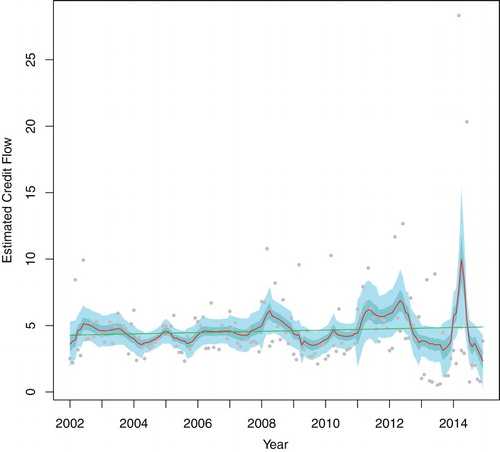
Figure 3 also shows approximate 50% and 95% pointwise confidence intervals for the credit flow trend. Interestingly, and not surprisingly, the variance of the trend estimate is slightly higher to the right of the plot, but due to the stability of the estimation procedure, the increase in variance is not markedly different across the plot.

The confidence intervals were obtained by bootstrap simulation in the transformed domain (using simulations from a simple ARMA error model added to the trend), inverting the transform and assuming approximate normality of the pointwise estimates. This is akin to the ‘simulating from the (wavelet) posterior’ mentioned in Barber et al. [2] or, more generally, Section 7.6 of [13], where we have a model for the transformed series, generate bootstrap samples from that model, invert each sample, and form pointwise confidence intervals from the samples thus generated in the original domain.

A similar trend plot could have been generated in a similar way for the log-transformation, but in view of the improved stabilisation of the data-driven Haar–Fisz transform observed in Figure 3(d) this seems unnecessary.

3. Forecasting

We next consider forecasting: an important task for budgeting and planning, see page 455 of [4]. Forecasting credit flows here enables decision makers to make use of information to lessen uncertainty and monitor volatile shipping environments, see page 701 of [58]. Forecasts are often discussed at board meetings and are usually supplemented with market information and expert opinion to form considered views about the current state of the industry. For budgeting, forecasts are used to assess likely expected revenues, expenses for future years and to help allocate financial resources. For strategic planning, forecasts are used to ascertain industry prospects and to help construct business plans with detailed policies. Frequently, forecasts form part of trade union negotiations and are also important within government, whose policies influence the industry's prospects.

To continue the previous analysis, we applied the exponential smoothing state space modelling function ets from the forecast package [33] to a large and contiguous training set of the transformed credit flow data (156−h observations) and then forecasted h steps ahead. Then, using the inverse transformation, we inverted the forecasts, and their nominal 95% prediction intervals, back to the original data domain for assessment. We compared the forecasts with the known truth both in terms of mean-squared prediction error and by computing empirical coverage of the forecasts. The ets methodology was selected because of its successful automatic general-purpose forecasting nature, see [32], although other alternatives might include the Box–Jenkins ARIMA methodology, or used in combination [39]. Other, more tailored computationally intensive smoothing methods [40] could be used to further improve forecasting performance.

Figure 4 shows four forecasts made for h=12 steps ahead using each of the four transformations. Of these, the data-driven Haar–Fisz method clearly has a prediction interval that covers most of the extreme values at the right-hand end of the plot. The Box–Cox and Log transforms' intervals are small and the square-root transformation not far behind. Clearly, the data-driven Haar–Fisz method could not have anticipated the huge values that were about to occur but it has obviously picked up on the increasing variance in the series prior to these.

Figure 5. Forecasts of Cyprus shipping credit flows for h=12 steps ahead obtained via four different transform methods. Grey line shows actual flow (as in Figure 1). Solid blue line shows the forecasts from one to h=12 steps ahead and the blue polygon shows the (nominal) 95% prediction interval.

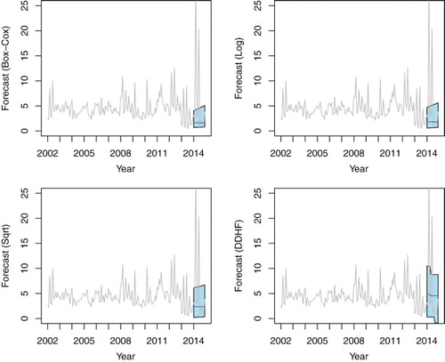
Table 1 shows the mean-squared prediction errors for the various forecasting horizons h ranging from three to 24. In six out of eight cases the data-driven Haar–Fisz transformed forecaster is either the best of within 2% of the best error. It is, however, not good for h=3,9 and, for the latter, considerably worse than the other three methods. Table 2 shows the empirical coverage of the nominal 95% prediction intervals: the data-driven Haar–Fisz method has the highest (or equal highest) coverage in six of the eight cases.

Table 1. Mean squared prediction error for the four transformations for varying forecasting horizons.

h	3	6	9	12	15	18	21	24
Box–Cox	0.86	1.21	1.98	2.73	2.19	1.76	1.50	1.35
Log	0.97	1.32	1.97	2.71	2.15	1.70	1.50	1.35
Sqrt	2.15	1.60	2.00	2.65	2.01	1.70	1.50	1.34
DDHF	1.96	1.23	3.44	2.46	2.05	1.70	1.48	1.37

Table 2. Empirical percentage coverage of 95% prediction intervals based on transformed ets forecasting based on eight different forecasting horizons, h.

h	3	6	9	12	15	18	21	24
Box–Cox	33	50	56	83	81	61	38	30
Log	66	50	56	83	81	50	48	33
Sqrt	33	50	56	83	53	50	43	46
DDHF	33	83	89	83	67	67	71	42

4. Discussion

The shipping credit flow problem is a particularly good exemplar for trend estimation and prediction with the data-driven Haar–Fisz transform because (i) the change in variance observed in the series is extreme (ii) existing powerful transformations singularly fail to stabilise the variance and (iii) the data-driven Haar–Fisz transform performs the stabilisation well and, further, gives interesting information as to the nature of the mean–variance relationship as shown by Figure 2.

Of course, there are several other paths that could have been followed to estimate trend. We could have fitted other time series trend models to the transformed data other than the smoothing spline (although this technique is well-understood and worked well), or fitted models other than ARIMA as part of our bootstrap confidence interval generator. There are alternative methods for handling the non-dyadic length of the data set and many other forecasting techniques that could have been tried. However, the aim of this case study is to clearly and directly set down a set of reasonable steps, with model justification at each step, to obtain a good estimator of the trend.

Further the techniques and analysis in this paper have been of direct use and genuinely useful in trend estimation and prediction for the credit flow (and other) shipping-related time series that are assessed by organisations such as the Central Bank of Cyprus as described by Michis and Nason [41].

The supplementary material contains the full R code of our analyses.

Acknowledgements

We thank T. Kazakos, Captain E. Adami and the Cyprus Shipping Chamber for helpful comments. The opinions expressed in this paper do not necessarily reflect the views of the Central Bank of Cyprus or the Eurosystem. The shipping credit flow data used in this paper is freely available in the DDHFm package for R available from the CRAN archive. The name of the data set is ShipCreditFlow.

Disclosure statement

No potential conflict of interest was reported by the authors.

Additional information

Funding

This research was supported by EPSRC Grant EP/K020951/1.

References

- A.P. Alencar, P.A. Morettin, and C.M.C. Toloi, State space Markov switching models using wavelets, Stud. Nonlinear Dyn. E. 17 (2013), pp. 221–238.
- S. Barber, G.P. Nason, and B.W. Silverman, Posterior probability intervals for wavelet thresholding, J. R. Stat. Soc. B 64 (2002), pp. 189–205.
- G.E.P. Box and D.R. Cox, An analysis of transformations (with discussion), J. R. Stat. Soc. B 26 (1964), pp. 211–252.
- A. Branch and M. Robarts, Branch's Elements of Shipping, 9th ed., Routledge, Abingdon, 2014.
- P.J. Brockwell and R.A. Davis, Time Series: Theory and Methods, Springer, New York, 1991.
- A. Cardinali and G.P. Nason, Costationarity of locally stationary time series, J. Time Ser. Econom. 2 (2010), Issue 2.
- A. Cardinali and G.P. Nason, Practical powerful wavelet packet tests for second-order stationarity, Appl. Comput. Harmon. Anal. 41 (2016), (to appear). DOI:doi: 10.1016/j.acha.2016.06.006.
- C. Chatfield, The Analysis of Time Series: An Introduction, 6th ed. Chapman and Hall/CRC, London, 2003.
- E.A.K. Cohen and A.T. Walden, A statistical analysis of temporally smoothed wavelet coherence, IEEE Trans. Signal Process 58 (2010), pp. 2964–2973.
- E.A.K. Cohen and A.T. Walden, Wavelet coherence for certain nonstationary bivariate processes, IEEE Trans. Signal Process 59 (2011), pp. 2522–2531.
- Cyprus Shipping Chamber, Annual report 2013, Limassol, Cyprus, 2014.
- R. Dahlhaus, Locally stationary processes, in Handbook of Statistics, T. Subba Rao, S. Subba Rao, and C. Rao, eds., Vol. 30, Elsevier, 2012, pp. 351–413.
- A.C. Davison and D.V. Hinkley, Bootstrap Methods and their Application, Cambridge University Press, Cambridge, 1997.
- H. Dette, P. Preuss, and M. Vetter, A measure of stationarity in locally stationary processes with applications to testing, J. Amer. Statist. Assoc. 106 (2011), pp. 1113–1124.
- J. Dickie, Reeds 21st Century Ship Management, Bloomsbury, London, 2014.
- Y. Dwivedi and Subba Rao S., A test for second-order stationarity of a time series based on the discrete Fourier transform, J. Time Ser. Anal. 32 (2011), pp. 68–91.
- I. Eckley, G. Nason, and R.L. Treloar, Locally stationary wavelet fields with application to the modelling and analysis of image texture, J. Roy. Statist. Soc. C 59 (2010), pp. 595–616.
- M. Fisz, The limiting distribution of a function of two independent random variables and its statistical application, Colloq. Math. 3 (1955), pp. 138–146.
- P.Z. Fryzlewicz, Wavelet techniques for time series and poisson data, Ph.D. thesis, University of Bristol, UK, 2003.
- P. Fryzlewicz, Modelling and forecasting financial log-returns as locally stationary wavelet processes, J. Appl. Stat. 32 (2005), pp. 503–528.
- P. Fryzlewicz, Data-driven wavelet-Fisz methodology for nonparametric function estimation, Electron. J. Stat. 2 (2008), pp. 863–896.
- P. Fryzlewicz, V. Delouille, and G.P. Nason, GOES-8 X-ray sensor variance stabilization using the multiscale data-driven Haar–Fisz transform., J. Roy. Statist. Soc. C 56 (2007), pp. 99–116.
- P. Fryzlewicz and G.P. Nason, A Haar–Fisz algorithm for Poisson intensity estimation, J. Comput. Graph. Statist. 13 (2004), pp. 621–638.
- P. Fryzlewicz and G.P. Nason, Haar–Fisz estimation of evolutionary wavelet spectra, J. R. Stat. Soc. B 68 (2006), pp. 611–634.
- P. Fryzlewicz and H. Ombao, Consistent classification of nonstationary time series using stochastic wavelet representations, J. Amer. Statist. Assoc. 104 (2009), pp. 299–312.
- P. Fryzlewicz, S. Van Bellegem, and R. von Sachs, Forecasting non-stationary time series by wavelet process modelling, Ann. Inst. Statist. Math. 55 (2003), pp. 737–764.
- W. Gardner and G. Zivanovic, Degrees of cyclostationarity and their application to signal detection and estimation, Signal Process. 22 (1991), pp. 287–297.
- A.J. Gibberd and J.D.B. Nelson, Regularised estimation of 2-d locally stationary wavelet processes, IEEE Statistical Signal Processing Workshop, 2016 (to appear). DOI:doi: 10.1109/SSP.2016.7551838.
- N.R. Goodman, Statistical tests for stationarity within the framework of harmonizable processes, Technical Report AD619270, Rockedyne, Canoga Park, CA, 1965.
- V. Guerrero, Time-series analysis supported by power transformations, J. Forecast. 12 (1993), pp. 37–48.
- H. Hurd and N. Gerr, Graphical methods for determining the presence of periodic correlation in time series, IEEE Trans. Inform. Theory 12 (1991), pp. 337–350.
- R. Hyndman, A. Koehler, R. Snyder, and S. Grose, A state space framework for automatic forecasting using exponential smoothing methods, Int. J. Forecast. 18 (2002), pp. 439–454.
- R. Hyndman, G. Athanasopoulos, S. Razbash, D. Schmidt, Z. Zhou, Y. Khan, C. Bergmeir, and E. Wang, Forecast: Forecasting Functions for Time Series and Linear Models, R Package Version 5.4, 2014.
- L. Jin, S. Wang, and H. Wang, A new non-parametric stationarity test of time series in the time domain, J. R. Stat. Soc. B 77 (2015), pp. 893–922.
- M.J. Keim and D.B. Percival, Assessing characteristic scales using wavelets, J. Roy. Statist. Soc. C 64 (2015), pp. 377–393.
- M. Knight and G.P. Nason, A nondecimated lifting transform, Stat. Comput. 19 (2009), pp. 1–16.
- M. Knight, G.P. Nason, and M.A. Nunes, A wavelet lifting approach to long-memory estimation, Stat. Comput. 26 (2016), (to appear), DOI:10.1007/s11222-016-9698-2.
- M.I. Knight, M.A. Nunes, and G.P. Nason, Spectral estimation for locally stationary time series with missing observations, Stat. Comput. 22 (2012), pp. 877–895.
- A. Michis, Do more forecasts always improve averages of model forecasts? Evidence from reports published by HM Treasury, OR Insight 26 (2013), pp. 234–241.
- A. Michis, A wavelet smoothing method to improve conditional sales forecasting, J. Oper. Res. Soc. 66 (2015), pp. 832–844.
- A.A. Michis and G.P. Nason, Estimation and prediction of shipping trends with the data-driven Haar-Fisz transform, Central Bank of Cyprus, Working Paper 2015–01, 2015.
- E. Motakis, G. Nason, and P. Fryzlewicz, DDHFm: Variance Stabilization by Data-Driven Haar–Fisz (for Microarrays), R Package Version 1.1.1, 2013.
- E.S. Motakis, G.P. Nason, P. Fryzlewicz, and G.A. Rutter, Variance stabilization and normalization for one-color microarray data using a data-driven multiscale approach, Bioinformatics 22 (2006), pp. 2547–2553.
- G.P. Nason, Stationary and non-stationary time series, in Statistics in Volcanology, H. Mader and S. Coles, eds., Geological Society of London, London, 2006, pp. 129–142.
- G.P. Nason, Wavelet Methods in Statistics with R, Springer, New York, 2008.
- G.P. Nason, A test for second-order stationarity and approximate confidence intervals for localized autocovariances for locally stationary time series., J. R. Stat. Soc. B 75 (2013), pp. 879–904.
- G.P. Nason, Multiscale variance stabilization via maximum likelihood, Biometrika 101 (2014), pp. 499–504.
- G.P. Nason and B.W. Silverman, The discrete wavelet transform in S, J. Comput. Graph. Statist. 3 (1994), pp. 163–191.
- G.P. Nason and R. von Sachs, Wavelets in time series analysis, Philos. Trans. R. Soc. Lond. A 357 (1999), pp. 2511–2526.
- G.P. Nason, R. von Sachs, and G. Kroisandt, Wavelet processes and adaptive estimation of the evolutionary wavelet spectrum, J. R. Stat. Soc. B 62 (2000), pp. 271–292.
- E. Paparoditis, Testing temporal constancy of the spectral structure of a time series, Bernoulli 15 (2009), pp. 1190–1221.
- E. Paparoditis, Validating stationarity assumptions in time series analysis by rolling local periodograms, J. Amer. Statist. Assoc. 105 (2010), pp. 839–851.
- D.B. Percival, A wavelet perspective on the Allan variance, IEEE Trans. Ultra. Ferro. Freq. Cont. 63 (2016), pp. 538–554.
- D.B. Percival and A.T. Walden, Wavelet Methods for Time Series Analysis, Cambridge University Press, Cambridge, 2000.
- M.B. Priestley, Spectral Analysis and Time Series, Academic Press, London, 1983.
- M.B. Priestley and Subba Rao T., A test for non-stationarity of time-series, J. R. Stat. Soc. B 31 (1969), pp. 140–149.
- R Development Core Team, R: A Language and Environment for Statistical Computing, R Foundation for Statistical Computing, Vienna, Austria, 2009, ISBN 3-900051-07-0.
- M. Stopford, Maritime Economics, Routledge, Abingdon, 2009.
- S.L. Taylor, I.A. Eckley, and M.A. Nunes, Multivariate locally stationary 2d wavelet processes with application to colour texture analysis, Stat. Comput. 26 (2016), to appear, DOI:10.1007/s11222-016-9675-9.
- K. Thon, M. Geilhufe, and D.B. Percival, A multiscale wavelet-based test for isotropy of random fields on a regular lattice, IEEE Trans. Image Process. 24 (2015), pp. 694–708.
- K. Triantafyllopoulos and G.P. Nason, A note on state-space representations of locally stationary wavelet time series, Statist. Probab. Lett. 79 (2008), pp. 50–54.
- S. Van Bellegem and R. von Sachs, On adaptive estimation for locally stationary wavelet processes and its applications, Int. J. Wavelets, Multiresolut. Inf. Process. 2 (2004), pp. 545–565.
- S. Van Bellegem and R. von Sachs, Locally adaptive estimation of evolutionary wavelet spectra, Ann. Statist. 36 (2008), pp. 1879–1924.
- R. von Sachs and B. MacGibbon, Non-parametric curve estimation by wavelet thresholding with locally stationary errors, Scand. J. Statist. 27 (2000), pp. 475–499.
- R. von Sachs and M.H. Neumann, A wavelet-based test for stationarity, J. Time Ser. Anal. 21 (2000), pp. 597–613.
- Y. Xie, J. Yu, and B. Ranneby, Forecasting using locally stationary wavelet processes, J. Stat. Comput. Simul. 79 (2009), pp. 1067–1082.
- B. Zhang, M.J. Fadili, and J.-L. Starck, Wavelets, ridgelets and curvelets for Poisson noise removal, IEEE Trans. Image Process. 17 (2008), pp. 1093–1108.