Application of machine learning approaches in the analysis of mass absorption cross-section of black carbon aerosols: Aerosol composition dependencies and sensitivity analyses

Abstract

Physics-based models typically require an in-depth understanding of a phenomenon and assumptions of the underlying process(es), which are often hard to obtain in practice, whereas data-driven machine learning models learn the structure and patterns in the training data without any prior theoretical assumptions and then use inference to develop useful predictions. A novel machine learning-based algorithm has been previously developed for the prediction of black carbon mass absorption cross-section (MAC_BC) and applied to a variety of different atmospheric environments. In contrast to light scattering theories which require assumptions about the underlying physics, this algorithm uses time-series data of aerosol properties to estimate the temporally varying MAC_BC at 870 nm. Here, we analyze our algorithm and discuss the influence of aerosol optical properties (such as Ångström exponents and single scattering albedo) and chemical composition on the model outputs and the associated accuracy. Additionally, we conduct sensitivity analyses on our models to understand how the predictions change in response to different sets of input variables. Our support vector machine (SVM) for regression model is the least sensitive to variations in the input variables, although all models tend to exhibit a degradation to their accuracy when scattering Ångström exponents are less than one.

This article is related to:

Estimating mass-absorption cross-section of ambient black carbon aerosols: Theoretical, empirical, and machine learning models

Introduction

Some of the first applications of machine learning in the field of aerosol science were related to the classification of single-particle mass spectrometer data (Zelenyuk et al. 2006; Murphy, Middlebrook, and Warshawsky 2003; Phares et al. 2001; Song et al. 1999). Over time, machine learning for aerosol classification has remained popular, for example, differentiation among bacteria, fungal spores, and pollen (Ruske et al. 2017); and classification of airborne metal particles (Davari and Wexler 2020). However, the emergence of data science and analytics has led to a growth in the popularity of other machine learning applications. These techniques have subsequently been applied to the prediction of aerosol microphysics (Zheng et al. 2021; Hughes et al. 2018) and cloud condensation nuclei concentrations (Nair and Yu 2020); the improvement of remote sensing retrievals (Zeng et al. 2020; Qin et al. 2018; Ma et al. 2011); the calibration or interpretation of low-cost particle sensor data (McFarlane et al. 2021; Patra et al. 2021; Si et al. 2020; Lim et al. 2019); the prediction of ambient black carbon (BC) concentrations (Fung et al. 2021; Abu Awad et al. 2017); and the correction of filter-based absorption photometer data (Kumar et al. 2022).

Our interest herein is black carbon (BC). Not only is BC relevant to human health, it has an important role in the climate system due to its ability to absorb solar radiation and to interact with clouds (Bond et al. 2013; Ramanathan and Carmichael 2008; Hansen, Rosen, and Novakov 1984). Traditionally, these phenomena have been modeled using physics-based light-scattering models within Earth system models (Wang et al. 2014; Myhre et al. 2013; Koch et al. 2009; Schulz et al. 2006), and these models require aerosol complex refractive indices, mixing state, size, and morphology as input variables (Liu et al. 2020; Forestieri et al. 2018; Zanatta et al. 2018; García Fernández, Picaud, and Devel 2015; Lack and Cappa 2010). These light-scattering models may have inherent uncertainties due to the necessary assumptions about the aerosol properties. However, the use of these models is necessary, because BC emissions are often mass-based (McDuffie et al. 2020; Bond et al. 2013), while the observations used to evaluate these Earth system models are often absorption-based. Even if one assumes a mass-absorption cross-section (MAC) to convert absorption to mass, values of MAC have been reported as variable across both time and space (Mbengue et al. 2021; Ohata et al. 2021; Yuan et al. 2021; Cho et al. 2019; Gyawali et al. 2017; Zanatta et al. 2016; Nordmann et al. 2013; Kondo et al. 2011; Moosmüller et al. 1998).

Recent efforts have applied machine learning to predict BC optical properties (Li and May 2020a; Luo et al. 2018) as an alternative to physics-based models. The inherent value of a viable statistical model for the prediction of BC optical properties is the potential to replace those physics-based light-scattering models, as the physics-based models may require major assumptions that are not constrained by empirical observations. In our previous work (Li and May 2020a), we presented the development and evaluation of regression and machine learning models for the prediction of the mass absorption cross-section of black carbon (MAC_BC, m² g⁻¹) at 870 nm. Briefly, these models use time-series data to predict temporal variations in MAC_BC using Python code that we have made publicly available (Li and May 2020b). Specifically, the models incorporate multi-wavelength aerosol light-absorption coefficients (B_abs, Mm⁻¹) and multi-wavelength aerosol light-scattering coefficients (B_scat, Mm⁻¹) along with information related to the particle number and volume distributions.

The challenge with all statistical models as candidates for replacing physics-based models is that they are inherently stochastic; therefore, they may struggle to represent physics-based deterministic problems, especially when extrapolation away from the training data occurs. However, if we can probe the limits of utility for a given statistical model, we can understand when a model will be inappropriate for use, potentially leading to subsequent improvements. In this study, we explore factors that may limit our models’ generalizability, namely, changes in aerosol composition and missing input data. In a separate companion study, we further explore how our models compare to physics-based models which explicitly account for aerosol complex refractive indices, mixing state, and morphology (Li and May 2022).

Methodology

Our approach to develop our regression and machine learning models is described in detail in Li and May (2020a). We provide a brief summary of this approach here.

Dataset description

We applied various regression and machine learning techniques to existing datasets. This included publicly available data from two US Department of Energy (DOE) Atmospheric Radiation Measurement (ARM) field campaigns: the Two-Column Aerosol Project (TCAP), which was conducted near Cape Cod, MA, US during 2012 − 2013; and the Cloud, Aerosol, and Complex Terrain Interactions (CACTI) project, which was conducted near Cordoba, Argentina during 2018 − 2019. We also included our data from the US National Oceanic and Atmospheric Administration Fire Influence on Regional to Global Environments Experiment (FIREX) that were collected at the US Forest Service Fire Science Laboratory in Missoula, MT, US in 2016.

Model inputs

For TCAP and CACTI, each modeling technique had the objective of predicting a time series of MAC_BC using time series of multi-wavelength B_abs, multi-wavelength B_scat, and parameterizations of both particle number and particle volume size distributions as inputs, while for FIREX, we used fire-integrated values. We focused on B_abs measured by filter-based absorption photometers, as these are more common in global atmospheric measurements than photoacoustic spectrometers. We corrected the B_abs data from these instruments using Li, McMeeking, and May (2020), which performs well both for ambient data collected at the US DOE ARM Southern Great Plains user facility and for our FIREX data. Our B_scat data were obtained from nephelometer measurements, and the particle size distributions were obtained from either a combination of a TSI Scanning Mobility Particle Sizer (SMPS) and a TSI Aerodynamic Particle Sizer (APS) or a stand-alone SMPS. Empirical values of MAC_BC at 870 nm were derived from B_abs at 870 nm and observed BC mass concentration (M_BC, µg m⁻³) from a Droplet Measurement Technologies Single Particle Soot Photometer (SP2), following Equation (1)(1) $$MA{C}_{BC}\left(870\mathrm{ }nm\right)=\frac{B_{\mathit{abs}}\left(870\mathrm{ }nm\right)}{M_{BC}}$$(1) : (1) $$MA{C}_{BC}\left(870\mathrm{ }nm\right)=\frac{B_{\mathit{abs}}\left(870\mathrm{ }nm\right)}{M_{BC}}$$(1) where we extended B_abs to 870 nm using empirically derived absorption Ångström exponents (AAE) from the multi-wavelength, filter-based absorption photometers measurements (i.e., B_abs ∼ λ^-AAE).

Modeling approach

The specific modeling techniques, considered in both Li and May (2020a) and here, included multiple linear regression using ordinary least squares (OLS); stepwise regression (both forward and backward); least absolute shrinkage and selection operation (LASSO); support vector machine for regression (SVM); artificial neural network (ANN); and one-dimensional convolutional neural network (CNN). We focus on the SVM for regression results in the main text, but we provide results for the other models in the online supplemental material.

The data were pre-processed using three separate modules: (1) to apply the correction algorithm from Li, McMeeking, and May (2020) to the B_abs data; (2) to merge the SMPS and APS data and to establish size distribution parameterizations; and (3) to adjust B_abs and B_scat to the “standard” wavelengths (467, 528, and 652 nm) using scattering Ångström exponents (SAE) and AAE, if needed. We conducted our data analysis using Python (version 3.7.5) for Windows in an “Anaconda” environment. We evaluated model performance using various metrics. This included the coefficient of determination (R²) and mean square error (MSE), as well as fractional bias and fractional error (Morris et al. 2005).

While we also included discussion using the Bond, Anderson, and Campbell (1999) correction algorithm, as updated by Ogren (2010), for B_abs in Li and May (2020a), we only focus on the corrections based on Li, McMeeking, and May (2020) within the present work, because the Li, McMeeking, and May (2020) correction algorithm yielded campaign-average MAC_BC values ranging between roughly 2.9 − 3.9 m² g⁻¹. This range is lower than, yet roughly consistent with, the expected MAC_BC of 4.7 m² g⁻¹ at 870 nm, based on the standard assumption of MAC_BC = 7.5 m² g⁻¹ at 550 nm from Bond and Bergstrom (2006) using an assumed AAE of 1, as in Lack and Langridge (2013). Conversely, the campaign-average MAC_BC values for the Bond, Anderson, and Campbell (1999) correction algorithm, as updated by Ogren (2010), ranged from 7.5 to 7.8 m² g⁻¹ at 870 nm (i.e., AAE is zero).

Results and discussion

We have presented a quantitative, statistical evaluation of our models in Li and May (2020a). Briefly, each model had similar performance between the training and test datasets (both from TCAP), but the quality of the performance with the training and test data varied among the models (cf., Table 4 and Figure 3 in Li and May [2020a]). Moreover, all models had “excellent” performance based on the fractional bias and fractional error criteria established by Morris et al. (2005) for the TCAP data (cf., Figure 3 in Li and May [2020a]). For the two independent validation datasets (CACTI and FIREX), the quality of the performance degraded for all models; R² decreased by at least a factor of two (from between ∼0.4 and ∼0.8 to <0.3), and MSE increased by roughly a factor of 10 (from ∼0.2 to ∼2) for all models. Moreover, the mean fractional error increased (from ∼0.1 to >0.3) for both datasets, while the fractional bias only increased for the CACTI data (from ∼0 to ∼0.1). Despite these limitations, all models performed better than the standard assumption (representing a constant value of MAC_BC) for both the time-series ambient data and the fire-integrated biomass burning data. Finally, we recommended that the SVM model should be used to calculate time series of MAC_BC for long-term field monitoring sites.

Several factors affecting model performance were alluded to but not fully explored within our previous work. One such effect was differences in aerosol composition that may exist when the models either under- or over-predicted the empirical values in the MAC_BC time series (cf., Figure 1c in Li and May [2020a]). Moreover, we wrote that “SVM is the least sensitive to variations in empirical limitations (e.g., if only a single wavelength of B_abs or B_scat is available, if only an APS is available)…” in Li and May (2020a). Here, we present how different aerosol composition affects the performance of our models and demonstrate the sensitivity of our models to missing input variables.

Influence of aerosol composition

To explore how different aerosol composition influences our models, we consider both direct measurements and inferences based on aerosol optical properties in our analysis. Due to differences in data availability, we separate this discussion into ambient aerosols and laboratory-generated biomass burning aerosols.

Ambient aerosols

For the two field campaigns studying ambient aerosols (TCAP and CACTI), there is available Aerodyne Aerosol Chemical Speciation Monitor (ACSM) data, which provides non-refractory sub-micron aerosol composition (i.e., ammonium, chloride, nitrate, organics, and sulfate); we primarily focus on the organic aerosol (OA) in this work. We use the derived SAE and AAE to interpret our results within the context of the “AAE-SAE” space proposed by Cazorla et al. (2013) and updated by Cappa et al. (2016), which can be used to estimate the type(s) of absorbing aerosols that are present in a given sample. For example, a sample that is dominated by mineral dust is expected to have high AAE yet low SAE, while a sample that is dominated by brown carbon (BrC) is likely to have both high AAE and high SAE. Furthermore, we use observations of B_scat and B_abs to derive values of single-scattering albedo (SSA), the ratio of light scattering to total light extinction (light scattering + light absorption).

In Figure 1, we present SAE and AAE data from TCAP (split into the training and test sets in panels (a) and (b), respectively) and CACTI (panel (c)), along with the classification scheme updated by Cappa et al. (2016) in panel (d). The markers in each of the panels represent hourly averages and are colored based on the ratio of the predicted MAC_BC at 870 nm from the SVM model to the empirically derived MAC_BC; if agreement falls within a factor of two (i.e., a ratio between 0.5 and 2.0, a subjective assessment), the values are grayed out to highlight discrepancies outside of this range (i.e., subjectively poor agreement). The square marker and error bars in the panels represent the mean and standard deviation of AAE and SAE for each dataset. When comparing across the three datasets, we note that the mean values of AAE and SAE at TCAP (1.54 and 1.36, respectively) are greater than those at CACTI (1.32 and 1.15, respectively). In addition, the CACTI data has large variations in SAE but smaller variations in AAE than the TCAP data. Complementary figures for the other models are presented in the online supporting information (Figures S1–S3). These figures provide a qualitative means of investigating how our models’ performance may vary on different ambient datasets with different types of absorbing aerosols present.

Figure 1. Hourly averaged AAE vs. SAE with points colored by the ratio of the SVM-predicted MAC_BC to the value derived from empirical observations for (a) training data; (b) test data; and (c) independent validation data. In panels (a)–(c), the square marker and error bars indicate the mean and standard deviation of the dataset; the filled circles represent over-predictions, and the filled triangles represent under-predictions. The classification scheme presented in Cappa et al. (2016) is shown in panel (d); this is overlaid onto panels (a)–(c).

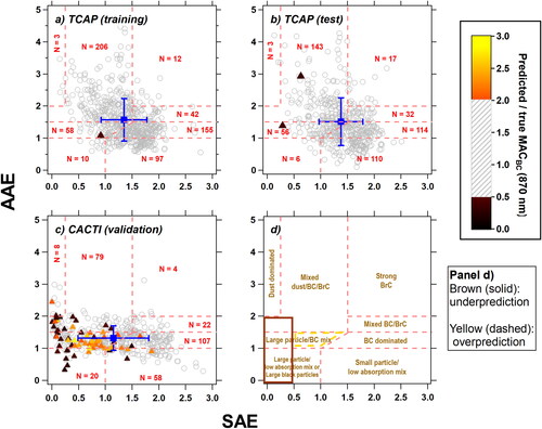
There are few colored markers for the data in Figures 1a and S1, suggesting that the models can predict the majority of these hourly averaged MAC_BC values from TCAP within a factor of two; this is not surprising because Figures 1a and S1 represent the training data for the models. This same observation holds true for Figures 1b and S2, which represent the test data from TCAP. However, for the CACTI data (Figures 1c and S3), more coloration appears, especially when SAE < 1; values tend to be over-predicted when SAE falls between 0.5 and 1.0 (the yellow region in Figure 1d), and they tend to be under-predicted when SAE < 0.5 (the brown region in Figure 1d). This is another result that is not entirely surprising, because there were relatively few observations for SAE < 1 and AAE < 1.5 in the training data. A comparison to the classification scheme in Figure 1d suggests that a substantial amount of large particles were present during the CACTI campaign, implying that our models for predicting MAC_BC may have limitations when, for example, mineral dust may dominate aerosol light absorption.

Figure 2. The ratio of the SVM-predicted MAC_BC to the value derived from empirical observations of MAC_BC as a function of (a) OA concentration; (b) BC concentration; and (c) SSA at 870 nm for the TCAP and CACTI data. The dashed line represents that the model fits MAC_BC.true without error.

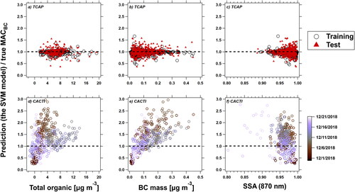
We next examine the association between model accuracy and measurements of aerosol composition. In Figure 2, we explore the influence of the mass concentrations of OA (from the ACSM) and BC (from the SP2) as well as SSA. The y-axis in each panel represents the ratio of the predicted MAC_BC at 870 nm from the model to the empirically derived value. In the top row, markers represent data from the TCAP campaign and are colored based on their inclusion as either training or test data; in the bottom row, markers represent data from the CACTI campaign and are colored based on date of collection. For the TCAP data, results are roughly normally-distributed about unity on the y-axis, with no clear systematic biases (cf., Table 4 and Figure 3 in Li and May [2020a]).

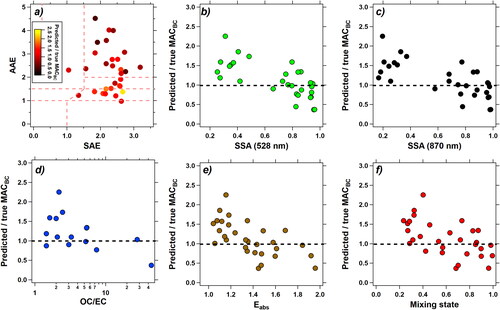
Figure 3. Association between the ratio of the SVM-predicted MAC_BC to the value derived from empirical observations to aerosol properties from the FIREX study. (a) The “AAE-SAE” space as in Figure 1; (b) SSA at 528 nm; (c) SSA at 870 nm; (d) the OC/EC ratio; (e) estimated E_abs; and (f) estimated mixing state. The dashed line in panels (b)–(f) represents a perfect agreement.

However, there is an apparent systematic bias in the CACTI data. The ratios tend to be less than unity at both the beginning (1 Dec 2018 through 3 Dec 2018) and the end (17 Dec 2018 through 21 Dec 2018) of the time-series data, which corresponded to OA concentrations less than roughly 3 µg m⁻³ and BC concentrations less than roughly 0.05 µg m⁻³; otherwise, the values tend to be biased high. Interestingly, the association between OA and BC concentrations (Figure S4) during CACTI is fairly strong (Pearson’s correlation coefficient r = 0.71), while this relationship is weak during TCAP (r = −0.09). The exact reason for this difference in the association between OA and BC between the two campaigns is unclear, but it may be related to differences in aerosol sources. For example, TCAP was likely dominated by marine aerosols and aerosols transported from continental North America (Kassianov et al. 2014) with a strong influence from aerosol hygroscopic growth (Titos et al. 2014). While we are unaware of any existing publications describing the source of the aerosols observed during CACTI, earlier work by Camponogara, Silva Dias, and Carrió (2014) suggests that the aerosols during this campaign likely originated from local sources, including biomass burning and wind-blown dust.

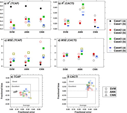
Figure 4. Statistical results of sensitivity analysis. The results of CNN applied to Case 3(a) and Case 3(b) for CACTI result in extreme prediction errors, so they fall outside of axis limits. The detailed results of R², MSE, and fractional bias and error can be found in Tables S1 and S2. Note the different scales in panels (a) and (b).

Moreover, meteorological conditions during the CACTI campaign favored convective storm development on some days (Schumacher et al. 2021; Varble et al. 2021), which is why the specific field site was selected. In fact, Schumacher et al. (2021) report lower maximum daily values of the most unstable convective available potential energy (MUCAPE), precipitable water, and vector wind difference (VWD) during the beginning and the end of the measurement period included in Figure 2. Schumacher et al. (2021) highlight that 13 Dec 2018 through 14 Dec 2018 had one of the largest MUCAPE/VWD combinations, which suggests the potential for severe convective storms. The presence of mesoscale convection may support an argument that the presence of wind-blown dust can result in the degradation of our models’ performance.

In addition to the variability of particle sources and meteorological conditions, we estimate that the BC particles at CACTI tend to have greater coating thickness than those at TCAP in complementary work (Li and May 2022); the accuracy of the machine learning models can be reduced by up to 50% if the ratio of coating mass to BC mass is greater than 20. Nevertheless, all of our models were able to predict the majority (>80%) of the empirically derived MAC_BC series within a factor of two, and they were generally able to capture temporal trends within those values.

Biomass burning aerosols

For the laboratory biomass burning aerosols (FIREX), we again interpret our data using the key optical parameters of aerosols (i.e., the AAE-SAE space and SSA). We did not have an ACSM co-located with our instrumentation (see Li et al. [2019] for details), but we do have organic carbon/elemental carbon (OC/EC) data from an offline Sunset Laboratories Lab OC/EC Aerosol Analyzer. Moreover, we have estimates of aerosol light absorption enhancement (E_abs) and a parameter representing the BC mixing state, both of which were derived from SP2 measurements, in these FIREX data; a value of 0 for the mixing state parameter indicates a pure external mixture, while a value of 1 indicates a pure internal mixture. Rather than time-series data, we present fire-integrated results for these data. Figure 3 illustrates the performance of the SVM model (see Figures S5–S6 for the other models).

In Figure 3a, no strong patterns related to biases in the SAE-AAE space emerge, suggesting that even though our training data did not contain a strong presence of BrC, the SVM model still exhibits good performance. Interestingly, the FIREX data do suggest an association between SSA and the ratio of the predicted MAC_BC at 870 nm from the model to the empirically derived value at both 528 nm (Figure 3b) and 870 nm (Figure 3c). A weaker association exists between the predicted-to-empirical MAC_BC ratio and the OC/EC ratio (Figure 3d), as we do not have OC/EC data for all fires, but there is no association between the predicted-to-empirical MAC_BC ratio and the absolute BC mass concentration from the SP2 (Figure S7). These observations for the FIREX data from Figures 3b–d and S5–S7 are in apparent direct contradiction to Figures 2d–f representing the CACTI data. However, the estimated aerosol light absorption enhancement (Figure 3e) and BC mixing state parameter (Figure 3f) mirrors the trends in Figures 3b–d, which is not surprising since SSA and the mixing state parameter are associated (Figure S8). Therefore, given the lack of a trend with SSA in Figure 2f, we postulate that BC mixing state, which will influence aerosol light absorption enhancement, is a key driver of biases in our models. Our SVM model appears to be the least sensitive to mixing state (e.g., compare Figure 3f with Figures S5–S6), as it predicts roughly 87% of the fire-integrated MAC_BC values within a factor of two. We further examine the influence of BC mixing state and aerosol light absorption enhancement in our companion study that incorporates physics-based light scattering modeling techniques into our analysis (Li and May 2022).

Sensitivity to varying model inputs

In addition to variations in aerosol composition that differ from the training dataset for our models, some observational sites may lack all of the input data required for our models. We consider here eight unique cases, all of which have practical implications, as summarized in Table 1. Case 1(a) is an exact reproduction of how we developed our models in Li and May (2020a) and serves as our base case, while Case 2(a) re-partitions the particle size distribution parameters using different electrical mobility diameter thresholds. Case 3(a) considers a scenario when only an SMPS (or equivalent) is available for particle sizing, and Case 4(a) considers a scenario when only an APS (or equivalent) is available for particle sizing. All cases denoted with a (b) consider only a single wavelength of B_abs and B_scat measurements but are otherwise identical to the analogous case denoted with an (a). Results in this section focus on the TCAP and CACTI datasets; we have effectively tested Case 3(a) in the previous section for the FIREX data, since only SMPS particle size distribution data were available during that campaign.

Table 1. Input variables considered in our sensitivity analyses. Multiple-λ includes information at 467, 528, and 652 nm, while single-λ only includes information at 528 nm. Values within the N_i and V_i columns represent the bounds of the particle size range (as electrical mobility diameter).

	Babs & Bscat	N1 (nm)	N2 (nm)	N3 (nm)	V1 (nm)	V2 (nm)	V3 (nm)	Notes
Case 1(a)	Multiple λ	< 50	50 − 200	> 200	< 1000	1000 − 2500	> 2500	SMPS and APS: 11.3 − 18,747 nm
Case 1(b)	Single λ	Same as Case 1(a)
Case 2(a)	Multiple λ	< 100	100 − 300	> 300	< 500	500 − 1500	> 1500	Repartitioning of size bins from Case 1(a)
Case 2(b)	Single λ	Same as Case 2(a)
Case 3(a)	Multiple λ	< 100	100 − 1000	–	< 500	500 − 1000	–	Emulating only an SMPS for sizing (< 1000 nm)
Case 3(b)	Single λ	Same as Case 3(a)
Case 4(a)	Multiple λ	–	440 − 600	> 600	–	440 − 2500	> 2500	Emulating only an APS for sizing (> 440 nm)
Case 4(b)	Single λ	Same as Case 4(a)

When conducting the sensitivity analyses, we directly input the variables generated by the cases presented in Table 1 to the trained models, and then compared the predicted MAC_BC against the empirical values of MAC_BC. Figure 4 presents a summary of the model performance metrics: R², MSE, fractional bias, and fractional error. As expected, this sensitivity analysis demonstrates that our models consistently perform worse on the TCAP data when inputs differ from the base case across all metrics. However, even though R² (Figure 4a) and MSE (Figure 4c) may differ by up to a factor of four from the base case in these TCAP data, most of the models can be still considered to be “excellent” with respect to fractional bias and fractional error (Figure 4e) based on the criteria established by Morris et al. (2005). Interestingly, for the CACTI dataset, all of the sensitivity analyses have similar (and sometimes improved) performance relative to the base case (Figures 4b, d, and f).

We can draw one important conclusion from Figure 4 and Tables S1–S2: the SVM model appears to be the least sensitive to changes in the input variables. For example, in Figures 4e and 4f, the SVM results (circles) tend to be clustered more tightly together for the sensitivity cases relative to the ANN (squares) and CNN (triangles) results for both datasets. The lower sensitivity of SVM is attributable to the inherent nature of the SVM training process. Fundamentally, the SVM approach selects a subset of observations from the training dataset as “support vectors” to define the margins of hyperplanes for the model (and to discard “unwanted” data samples), which makes the model robust to data noise and applicable to datasets with substitution of input variables. Therefore, even if input data are missing relative to the training data, this model can still perform reasonably well. This analysis supports our previous recommendation for the use of the SVM model for predicting MAC_BC from empirical data.

Conclusions and extensions

We have expanded upon the evaluation of our machine learning models that were developed to calculate MAC_BC based on multi-wavelength B_abs, multi-wavelength B_scat, and parameterizations of both particle number and particle volume size distributions. Specifically, we considered the influence of varying composition and the effect that this has on the accuracy of our model predictions. While our machine learning models generally perform well, there are some scenarios for which their performance degrades. When mineral dust (Figure 1c) or externally mixed BC (Figure 2f) particles dominate aerosol light absorption, the bias in the models can exceed a factor of two. Therefore, MAC_BC predictions with our models for observational sites influenced by wind-blown dust or freshly generated BC particles may be prone to errors, because our models are extrapolating for those calculations. However, two advantages of our models are that they do not require assumptions on aerosol composition or mixing state (e.g., as in physics-based light scattering models) and that they can capture temporal variations in MAC_BC (unlike the constant, standard assumption of MAC_BC); we specifically compare our SVM model to these other approaches in a companion study (Li and May 2022).

We envision several extensions to our work that either we or other researchers may pursue in the future. We have focused on the development of a generalizable model that may be applied to any site globally. However, there may be specific applications of our model that are very different from our original training dataset (cf., Table 1 in Li and May [2020a], Figure 1a above), which lead to poor model performance. To overcome this issue, one could re-train our model using a dataset representing a more diverse aerosol population that is more widely generalizable. Alternatively, one could conduct short-term intensive field campaigns to develop site-specific machine-learning models; this would also provide additional data that could be used to evaluate our generalized model. Moreover, we have developed three pre-processing modules that enable users to process raw observations into the required data format used in our model. Our existing modules may be useful in standalone applications. Likewise, we focused on these three as they served our needs in the development of our machine-learning models, but extensions to our work could lead to the development of additional modules.

Supplementary information

Additional figures and tables are available with the online publication. Computer code is available from https://zenodo.org/record/3967833. The TCAP and CACTI aerosol products are available at https://www.archive.arm.gov/discovery/. The FIREX data are available at https://www.esrl.noaa.gov/csl/projects/firex/firelab/.

Additional information

Funding

This work was funded by the Atmospheric Chemistry, Carbon Cycle, & Climate program within the National Oceanic and Atmospheric Administration’s Climate Program Office through award NA16OAR4310109. The ambient data at the TCAP and CACTI sites were obtained from the Atmospheric Radiation Measurement (ARM) user facility, a U.S. Department of Energy (DOE) Office of Science user facility managed by the Office of Biological and Environmental Research.

References

- Abu Awad, Y., P. Koutrakis, B. A. Coull, and J. Schwartz. 2017. A spatio-temporal prediction model based on support vector machine regression: Ambient black carbon in three New England States. Environ. Res. 159:427–34. doi:10.1016/j.envres.2017.08.039.
- Bond, T. C., T. L. Anderson, and D. Campbell. 1999. Calibration and intercomparison of filter-based measurements of visible light absorption by aerosols. Aerosol Sci. Technol. 30 (6):582–600. doi:10.1080/027868299304435.
- Bond, T. C, and R. W. Bergstrom. 2006. Light absorption by carbonaceous particles: An investigative review. Aerosol Sci. Technol. 40 (1):27–67. doi:10.1080/02786820500421521.
- Bond, T. C., S. J. Doherty, D. W. Fahey, P. M. Forster, T. Berntsen, B. J. DeAngelo, M. G. Flanner, S. Ghan, B. Kärcher, D. Koch, et al. 2013. Bounding the role of black carbon in the climate system: A scientific assessment. J. Geophys. Res. Atmos. 118 (11):5380–552. doi:10.1002/jgrd.50171.
- Camponogara, G., M. A. F. Silva Dias, and G. G. Carrió. 2014. Relationship between Amazon biomass burning aerosols and rainfall over the La Plata Basin. Atmos. Chem. Phys. 14 (9):4397–407. doi:10.5194/acp-14-4397-2014.
- Cappa, C. D., K. R. Kolesar, X. Zhang, D. B. Atkinson, M. S. Pekour, R. A. Zaveri, A. Zelenyuk, and Q. Zhang. 2016. Understanding the optical properties of ambient sub- and supermicron particulate matter: Results from the CARES 2010 field study in northern California. Atmos. Chem. Phys. 16 (10):6511–35. doi:10.5194/acp-16-6511-2016.
- Cazorla, A., R. Bahadur, K. J. Suski, J. F. Cahill, D. Chand, B. Schmid, V. Ramanathan, and K. A. Prather. 2013. Relating aerosol absorption due to soot, organic carbon, and dust to emission sources determined from in-situ chemical measurements. Atmos. Chem. Phys. 13 (18):9337–50. doi:10.5194/acp-13-9337-2013.
- Cho, C., S.-W. Kim, M. Lee, S. Lim, W. Fang, Ö. Gustafsson, A. Andersson, R. J. Park, and P. J. Sheridan. 2019. Observation-based estimates of the mass absorption cross-section of black and brown carbon and their contribution to aerosol light absorption in East Asia. Atmos. Environ. 212:65–74. doi:10.1016/j.atmosenv.2019.05.024.
- Davari, S. A, and A. S. Wexler. 2020. Quantification of toxic metals using machine learning techniques and spark emission spectroscopy. Atmos. Meas. Tech. 13 (10):5369–77. doi:10.5194/amt-13-5369-2020.
- Forestieri, S. D., T. M. Helgestad, A. T. Lambe, L. Renbaum-Wolff, D. A. Lack, P. Massoli, E. S. Cross, M. K. Dubey, C. Mazzoleni, J. S. Olfert, et al. 2018. Measurement and modeling of the multiwavelength optical properties of uncoated flame-generated soot. Atmos. Chem. Phys. 18 (16):12141–59. doi:10.5194/acp-18-12141-2018.
- Fung, P. L., M. A. Zaidan, H. Timonen, J. V. Niemi, A. Kousa, J. Kuula, K. Luoma, S. Tarkoma, T. Petäjä, M. Kulmala, et al. 2021. Evaluation of white-box versus black-box machine learning models in estimating ambient black carbon concentration. J. Aerosol Sci 152:105694. doi:10.1016/j.jaerosci.2020.105694.
- García Fernández, C., S. Picaud, and M. Devel. 2015. Calculations of the mass absorption cross sections for carbonaceous nanoparticles modeling soot. J. Quant. Spectrosc. Radiat. Transf. 164:69–81. doi:10.1016/j.jqsrt.2015.05.011.
- Gyawali, M., W. P. Arnott, R. Zaveri, C. Song, B. Flowers, M. Dubey, A. Setyan, Q. Zhang, S. China, C. Mazzoleni, et al. 2017. Evolution of multispectral aerosol absorption properties in a biogenically-influenced urban environment during the CARES campaign. Atmosphere (Basel) 8 (12):217. doi:10.3390/atmos8110217.
- Hansen, A. D. A., H. Rosen, and T. Novakov. 1984. The aethalometer—An instrument for the real-time measurement of optical absorption by aerosol particles. Sci. Total Environ. 36:191–6. doi:10.1016/0048-9697(84)90265-1.
- Hughes, M., J. Kodros, J. Pierce, M. West, and N. Riemer. 2018. Machine learning to predict the global distribution of aerosol mixing state metrics. Atmosphere (Basel) 9 (1):15. doi:10.3390/atmos9010015.
- Kassianov, E., J. Barnard, M. Pekour, L. K. Berg, J. Shilling, C. Flynn, F. Mei, and A. Jefferson. 2014. Simultaneous retrieval of effective refractive index and density from size distribution and light-scattering data: Weakly absorbing aerosol. Atmos. Meas. Tech. 7 (10):3247–61. doi:10.5194/amt-7-3247-2014.
- Koch, D., M. Schulz, S. Kinne, C. McNaughton, J. R. Spackman, Y. Balkanski, S. Bauer, T. Berntsen, T. C. Bond, O. Boucher, et al. 2009. Evaluation of black carbon estimations in global aerosol models. Atmos. Chem. Phys. 9 (22):9001–26. doi:10.5194/acp-9-9001-2009.
- Kondo, Y., H. Matsui, N. Moteki, L. Sahu, N. Takegawa, M. Kajino, Y. Zhao, M. J. Cubison, J. L. Jimenez, S. Vay, et al. 2011. Emissions of black carbon, organic, and inorganic aerosols from biomass burning in North America and Asia in 2008. J. Geophys. Res. 116 (D8):D16302. doi:10.1029/2010JD015152.
- Kumar, J., T. Paik, N. Shetty, P. Sheridan, A. Aiken, M. Dubey, and R. Chakrabarty. 2022. Correcting for filter-based aerosol light absorption biases at ARM’s SGP site using photoacoustic data and machine learning. Atmos. Meas. Tech. 15 (15):4569–83. doi:10.5194/amt-2022-42.
- Lack, D. A, and C. D. Cappa. 2010. Impact of brown and clear carbon on light absorption enhancement, single scatter albedo and absorption wavelength dependence of black carbon. Atmos. Chem. Phys. 10 (9):4207–20. doi:10.5194/acp-10-4207-2010.
- Lack, D. A, and J. M. Langridge. 2013. On the attribution of black and brown carbon light absorption using the Ångström exponent. Atmos. Chem. Phys. 13 (20):10535–43. doi:10.5194/acp-13-10535-2013.
- Li, H., K. D. Lamb, J. P. Schwarz, V. Selimovic, R. J. Yokelson, G. R. McMeeking, and A. A. May. 2019. Inter-comparison of black carbon measurement methods for simulated open biomass burning emissions. Atmos. Environ. 206:156–69. doi:10.1016/j.atmosenv.2019.03.010.
- Li, H, and A. A. May. 2022. Estimating absorption cross section of ambient black carbon aerosols: Theoretical, empirical, and machine learning models. Aerosol Sci. Technol. doi:10.1080/02786826.2022.2114311.
- Li, H, and A. A. May. 2020a. An exploratory approach using regression and machine learning in the analysis of mass absorption cross section of black carbon aerosols: Model development and evaluation. Atmosphere (Basel). 11 (11):1185. doi:10.3390/atmos11111185.
- Li, H, and A. A. May. 2020b. Application of regression and machine learning approaches in the analysis of mass absorption cross section of black carbon aerosols. Zenodo. https://zenodo.org/record/3967833. doi:10.5281/zenodo.3967833.
- Li, H., G. R. McMeeking, and A. A. May. 2020. Development of a new correction algorithm applicable to any filter-based absorption photometer. Atmos. Meas. Tech. 13 (5):2865–86. doi:10.5194/amt-13-2865-2020.
- Lim, C. C., H. Kim, M. J. R. Vilcassim, G. D. Thurston, T. Gordon, L.-C. Chen, K. Lee, M. Heimbinder, and S.-Y. Kim. 2019. Mapping urban air quality using mobile sampling with low-cost sensors and machine learning in Seoul, South Korea. Environ. Int. 131:105022. doi:10.1016/j.envint.2019.105022.
- Liu, F., J. Yon, A. Fuentes, P. Lobo, G. J. Smallwood, and J. C. Corbin. 2020. Review of recent literature on the light absorption properties of black carbon: Refractive index, mass absorption cross section, and absorption function. Aerosol Sci. Technol. 54 (1):33–51. doi:10.1080/02786826.2019.1676878.
- Luo, J., Y. Zhang, F. Wang, J. Wang, and Q. Zhang. 2018. Applying machine learning to estimate the optical properties of black carbon fractal aggregates. J. Quant. Spectrosc. Radiat. Transf. 215:1–8. doi:10.1016/j.jqsrt.2018.05.002.
- Ma, Y., W. Gong, P. Wang, and X. Hu. 2011. New dust aerosol identification method for spaceborne lidar measurements. J. Quant. Spectrosc. Radiat. Transf. 112 (2):338–45. doi:10.1016/j.jqsrt.2010.08.004.
- Mbengue, S., N. Zikova, J. Schwarz, P. Vodička, A. H. Šmejkalová, and I. Holoubek. 2021. Mass absorption cross-section and absorption enhancement from long term black and elemental carbon measurements: A rural background station in Central Europe. Sci. Total Environ. 794:148365. doi:10.1016/j.scitotenv.2021.148365.
- McDuffie, E. E., S. J. Smith, P. O'Rourke, K. Tibrewal, C. Venkataraman, E. A. Marais, B. Zheng, M. Crippa, M. Brauer, and R. V. Martin. 2020. A global anthropogenic emission inventory of atmospheric pollutants from sector- and fuel-specific sources (1970–2017): An application of the community emissions data system (CEDS). Earth Syst. Sci. Data 12 (4):3413–42. doi:10.5194/essd-12-3413-2020.
- McFarlane, C., G. Raheja, C. Malings, E. K. E. Appoh, A. F. Hughes, and D. M. Westervelt. 2021. Application of Gaussian mixture regression for the correction of low cost PM 2.5 monitoring data in Accra, Ghana. ACS Earth Space Chem. 5 (9):2268–79. doi:10.1021/acsearthspacechem.1c00217.
- Moosmüller, H., W. P. Arnott, C. F. Rogers, J. C. Chow, C. A. Frazier, L. E. Sherman, and D. L. Dietrich. 1998. Photoacoustic and filter measurements related to aerosol light absorption during the Northern Front Range air quality study (Colorado 1996/1997). J. Geophys. Res. 103 (D21):28149–57. doi:10.1029/98JD02618.
- Morris, R. E., D. E. McNally, T. W. Tesche, G. Tonnesen, J. W. Boylan, and P. Brewer. 2005. Preliminary evaluation of the community multiscale air quality model for 2002 over the Southeastern United States. J. Air Waste Manag. Assoc. 55 (11):1694–708. doi:10.1080/10473289.2005.10464765.
- Murphy, D. M., A. M. Middlebrook, and M. Warshawsky. 2003. Cluster analysis of data from the particle analysis by laser mass spectrometry (PALMS) instrument. Aerosol Sci. Technol. 37 (4):382–91. doi:10.1080/02786820300971.
- Myhre, G., B. H. Samset, M. Schulz, Y. Balkanski, S. Bauer, T. K. Berntsen, H. Bian, N. Bellouin, M. Chin, T. Diehl, et al. 2013. Radiative forcing of the direct aerosol effect from AeroCom Phase II simulations. Atmos. Chem. Phys. 13 (4):1853–77. doi:10.5194/acp-13-1853-2013.
- Nair, A. A, and F. Yu. 2020. Using machine learning to derive cloud condensation nuclei number concentrations from commonly available measurements. Atmos. Chem. Phys. 20 (21):12853–69. doi:10.5194/acp-20-12853-2020.
- Nordmann, S., W. Birmili, K. Weinhold, K. Müller, G. Spindler, and A. Wiedensohler. 2013. Measurements of the mass absorption cross section of atmospheric soot particles using Raman spectroscopy. J. Geophys. Res. Atmos. 118 (21):12075–12085. doi:10.1002/2013JD020021.
- Ogren, J. A. 2010. Comment on “Calibration and Intercomparison of Filter-Based Measurements of Visible Light Absorption by Aerosols”. Aerosol Sci. Technol 44 (8):589–91. doi:10.1080/02786826.2010.482111.
- Ohata, S., T. Mori, Y. Kondo, S. Sharma, A. Hyvärinen, E. Andrews, P. Tunved, E. Asmi, J. Backman, H. Servomaa, et al. 2021. Estimates of mass absorption cross sections of black carbon for filter-based absorption photometers in the Arctic. Atmos. Meas. Tech. 14 (10):6723–48. doi:10.5194/amt-14-6723-2021.
- Patra, S. S., R. Ramsisaria, R. Du, T. Wu, and B. E. Boor. 2021. A machine learning field calibration method for improving the performance of low-cost particle sensors. Build. Environ 190:107457. doi:10.1016/j.buildenv.2020.107457.
- Phares, D. J., K. P. Rhoads, A. S. Wexler, D. B. Kane, and M. V. Johnston. 2001. Application of the ART-2a algorithm to laser ablation aerosol mass spectrometry of particle standards. Anal. Chem. 73 (10):2338–44. doi:10.1021/ac0015063.
- Qin, W., L. Wang, A. Lin, M. Zhang, and M. Bilal. 2018. Improving the estimation of daily aerosol optical depth and aerosol radiative effect using an optimized artificial neural network. Remote Sens. 10 (7):1022. doi:10.3390/rs10071022.
- Ramanathan, V, and G. Carmichael. 2008. Global and regional climate changes due to black carbon. Nature Geosci. 1 (4):221–7. doi:10.1038/ngeo156.
- Ruske, S., D. O. Topping, V. E. Foot, P. H. Kaye, W. R. Stanley, I. Crawford, A. P. Morse, and M. W. Gallagher. 2017. Evaluation of machine learning algorithms for classification of primary biological aerosol using a new UV-LIF spectrometer. Atmos. Meas. Tech. 10 (2):695–708. doi:10.5194/amt-10-695-2017.
- Schulz, M., C. Textor, S. Kinne, Y. Balkanski, S. Bauer, T. Berntsen, T. Berglen, O. Boucher, F. Dentener, S. Guibert, et al. 2006. Radiative forcing by aerosols as derived from the AeroCom present-day and pre-industrial simulations. Atmos. Chem. Phys. 6 (12):5225–46. doi:10.5194/acpd-6-5095-2006.
- Schumacher, R. S., D. A. Hence, S. W. Nesbitt, R. J. Trapp, K. A. Kosiba, J. Wurman, P. Salio, M. Rugna, A. C. Varble, and N. R. Kelly. 2021. Convective-storm environments in subtropical South America from high-frequency soundings during RELAMPAGO-CACTI. Mon. Weather Rev 149 (5):1439–58. doi:10.1175/MWR-D-20-0293.1.
- Si, M., Y. Xiong, S. Du, and K. Du. 2020. Evaluation and calibration of a low-cost particle sensor in ambient conditions using machine-learning methods. Atmos. Meas. Tech. 13 (4):1693–707. doi:10.5194/amt-13-1693-2020.
- Song, X.-H., P. K. Hopke, D. P. Fergenson, and K. A. Prather. 1999. Classification of single particles analyzed by ATOFMS using an artificial neural network, ART-2A. Anal. Chem. 71 (4):860–5. doi:10.1021/ac9809682.
- Titos, G., A. Jefferson, P. J. Sheridan, E. Andrews, H. Lyamani, L. Alados-Arboledas, and J. A. Ogren. 2014. Aerosol light-scattering enhancement due to water uptake during the TCAP campaign. Atmos. Chem. Phys. 14 (13):7031–43. doi:10.5194/acp-14-7031-2014.
- Varble, A. C., S. W. Nesbitt, P. Salio, J. C. Hardin, N. Bharadwaj, P. Borque, P. J. DeMott, Z. Feng, T. C. J. Hill, J. N. Marquis, et al. 2021. Utilizing a storm-generating hotspot to study convective cloud transitions: The CACTI experiment. Bull. Am. Meteorol. Soc. 102 (8):E1597–E1620. doi:10.1175/BAMS-D-20-0030.1.
- Wang, X., C. L. Heald, D. A. Ridley, J. P. Schwarz, J. R. Spackman, A. E. Perring, H. Coe, D. Liu, and A. D. Clarke. 2014. Exploiting simultaneous observational constraints on mass and absorption to estimate the global direct radiative forcing of black carbon and brown carbon. Atmos. Chem. Phys. 14 (20):10989–1010. doi:10.5194/acp-14-10989-2014.
- Yuan, J., R. L. Modini, M. Zanatta, A. B. Herber, T. Müller, B. Wehner, L. Poulain, T. Tuch, U. Baltensperger, and M. Gysel-Beer. 2021. Variability in the mass absorption cross section of black carbon (BC) aerosols is driven by BC internal mixing state at a central European background site (Melpitz, Germany) in winter. Atmos. Chem. Phys. 21 (2):635–55. doi:10.5194/acp-21-635-2021.
- Zanatta, M., M. Gysel, N. Bukowiecki, T. Müller, E. Weingartner, H. Areskoug, M. Fiebig, K. E. Yttri, N. Mihalopoulos, G. Kouvarakis, et al. 2016. A European aerosol phenomenology-5: Climatology of black carbon optical properties at 9 regional background sites across Europe. Atmos. Environ. 145:346–64. doi:10.1016/j.atmosenv.2016.09.035.
- Zanatta, M., P. Laj, M. Gysel, U. Baltensperger, S. Vratolis, K. Eleftheriadis, Y. Kondo, P. Dubuisson, V. Winiarek, S. Kazadzis, et al. 2018. Effects of mixing state on optical and radiative properties of black carbon in the European Arctic. Atmos. Chem. Phys. 18 (19):14037–57. doi:10.5194/acp-18-14037-2018.
- Zelenyuk, A., D. Imre, Y. Cai, K. Mueller, Y. Han, and P. Imrich. 2006. SpectraMiner, an interactive data mining and visualization software for single particle mass spectroscopy: A laboratory test case. Int. J. Mass Spectrom 258 (1–3):58–73. doi:10.1016/j.ijms.2006.06.015.
- Zeng, S., A. Omar, M. Vaughan, M. Ortiz, C. Trepte, J. Tackett, J. Yagle, P. Lucker, Y. Hu, D. Winker, et al. 2020. Identifying aerosol subtypes from CALIPSO lidar profiles using deep machine learning. Atmosphere (Basel 12 (1):10. doi:10.3390/atmos12010010.
- Zheng, Z., J. H. Curtis, Y. Yao, J. T. Gasparik, V. G. Anantharaj, L. Zhao, M. West, and N. Riemer. 2021. Estimating submicron aerosol mixing state at the global scale with machine learning and earth system modeling. Earth Sp. Sci 8 (2):e2020EA001500. doi:10.1029/2020EA001500.