Conflict forecasting with event data and spatio-temporal graph convolutional networks

Abstract

This paper explores three different model components to improve predictive performance over the ViEWS benchmark: a class of neural networks that account for spatial and temporal dependencies; the use of CAMEO-coded event data; and the continuous rank probability score (CRPS), which is a proper scoring metric. We forecast changes in state based violence across Africa at the grid-month level. The results show that spatio-temporal graph convolutional neural network models offer consistent improvements over the benchmark. The CAMEO-coded event data sometimes improve performance, but sometimes decrease performance. Finally, the choice of performance metric, whether it be the mean squared error or a proper metric such as the CRPS, has an impact on model selection. Each of these components–algorithms, measures, and metrics–can improve our forecasts and understanding of violence.

En este artículo se exploran tres componentes diferentes del modelo para mejorar el rendimiento predictivo con respecto a la referencia ViEWS: una clase de redes neuronales que tienen en cuenta las dependencias espaciales y temporales, el uso de datos de eventos codificados por CAMEO, y la puntuación de probabilidad de rango continuo (CRPS), que es una métrica de puntuación adecuada. Predecimos los cambios en la violencia estatal en toda África a nivel mensual. Los resultados muestran que los modelos de redes neuronales convolucionales de gráficos espacio-temporales ofrecen mejoras consistentes sobre el punto de referencia. Los datos de eventos codificados por CAMEO a veces mejoran el rendimiento, pero otras veces lo empeoran. Por último, la elección de la métrica de rendimiento, ya sea el error cuadrático medio o una métrica propia como la CRPS, influye en la selección del modelo. Cada uno de estos componentes (algoritmos, medidas y métricas) puede mejorar nuestras previsiones y nuestra comprensión de la violencia.

Cet article explore trois composantes de modèles différentes pour améliorer les performances prédictives par rapport à la référence de ViEWS (Violence early-warning system, système d’alerte précoce sur la violence) : une classe de réseaux de neurones qui prennent en compte les dépendances spatiales et temporelles ; l’utilisation de données d’événements codées par CAMEO (Conflict and Mediation Events Observations, Observation des événements de médiation et de conflit) ; et le CRPS (Continuous Rank Probability Score, Score de probabilité de catégories ordonnées de variables continues), qui est une métrique de score propre. Nous effectuons des prédictions des évolutions de la violence étatique en Afrique au niveau grille/mois. Les résultats montrent que les modèles à réseaux convolutifs de neurones graphiques spatiotemporels offrent des améliorations constantes par rapport à la référence. Les données d’événements codées par CAMEO améliorent parfois les performances mais peuvent aussi parfois les réduire. Enfin, le choix de la métrique de performances, qu’il s’agisse de l’erreur quadratique moyenne ou d’une métrique de score propre telle que le CRPS, a un impact sur la sélection du modèle. Chacune de ces composantes - algorithmes, mesures et métriques - peut améliorer nos prévisions et notre compréhension de la violence.

Keywords:

• Conflict forecasting
• event data
• methodology

View correction statement:

Correction

Introduction

Our approach to improving the prediction of fatalities in the PRIO-GRID focuses on three major model components: the input data for the model, the learning algorithm, and the forecast evaluation metrics. We focus on monthly-grid level predictions for Africa. Our results show that the spatio-temporal graph convolutional neural network improves predictive performance over the benchmark. The choice of performance metric matters, as model selection and inferences drawn, can vary by metric. Finally, event data sometimes improves performance, and sometimes decreases performance.

Conflict dynamics tend to show strong spatial and temporal auto-correlation as violence usually clusters in conflict-prone spaces and temporal inertias tend to contribute to sustained waves of violence (Berman et al. 2017; Buhaug and Gleditsch 2008; Findley and Young 2012). Given the dependencies of conflict over time and across space, conflict forecasting models exhibit many non-linear relationships as well as spatial and temporal auto-correlation (D’Orazio 2020). Researchers have employed different machine learning and regression techniques to account for these attributes (Beck, King, and Zeng 2000; Hill and Jones 2014; Cranmer and Desmarais 2017). Yet, there is no consensus on the best modeling approach, and researchers are constantly innovating to improve predictive performance (Dorff, Gallop, and Minhas 2020). In this paper, we introduce the spatio-temporal graph convolutional neural networks (ST-GCN), which is highly flexible and can account for spatial and temporal dependencies, to predict conflict dynamics at the monthly-grid level for Africa. Additionally, we focus on building an end-to-end framework with minimal feature engineering, which means that all inputs to the model are raw features, as shown in supplemental materials. The results show consistent improvements over the benchmark models.

In addition to the standard variables in the benchmark ViEWS fatality model, we add monthly ICEWS event data, which are available back to 1995 (Boschee et al. 2015). We expect that the fine-grained and rapidly changing nature of event data can contribute to improve forecasting performance. While some research has shown that ICEWS does not always lead to improvements in predictive performance (Chiba and Gleditsch 2017), others have shown successful applications of the ICEWS data for forecasting civil conflict when the features constructed from the raw event data are theoretically informed (Blair and Sambanis 2020). ICEWS codes events using the Conflict and Mediation Event Observations (CAMEO) framework (Gerner, Schrodt, and Yilmaz 2009), which is a widely-used coding scheme for event data that was optimized for studying third-party mediation in international disputes. CAMEO was based in part on WEIS, but designed to code events that are relevant to mediating violent conflict and to be a framework that categorizes a broad set of political interactions (McClelland 1976; Schrodt 2012). In this application, we use CAMEO event counts aggregated by root code for each grid cell month, and rely on the flexibility of our modeling technique to capture the important relationships between fatalities and ICEWS events. The different models specifications show these event data sometimes improve performance, but sometimes undermine the predictive performance of the models. This assessment depends on choice of performance metric.

Our third contribution to improve these predictive models of conflict is to consider the continuous rank probability score (CRPS) as a model performance metric (Hersbach 2000). The CRPS is a proper scoring metric that accounts for the distribution of the prediction, not only the point prediction, as is the case with mean squared error (Brandt, Freeman, and Schrodt 2014). This metric can improve model selection, and account for the full distribution. The results show that the choice of metric, whether mean squared error (MSE) or CRPS, has an effect on the conclusions.

Related Work

A brief review of time-series forecasting is presented to provide general information about methods to model sequential data. Then, we discuss deep learning, spatio-temporal models to address the sequential modeling problem.

Time-Series Forecasting

Conventional machine learning algorithms for time series forecasting are normally divided into two categories: traditional methods, and deep learning methods (Wang et al. 2020). Traditional time-series forecasting models include Auto Regressive Integrated Moving Average (ARIMA) and Random Forests regression. Although these two methods allow for non-stationary patterns in a time series, they generally do not capture the long-term dependencies within the sequence (Siami-Namini, Tavakoli, and Namin 2018; Kane et al. 2014).

The recent implementation of deep neural networks to time-series prediction has pushed the performance of sequential modeling to a new level. There are two major types of networks that are widely used. Recurrent Neural Network (RNN) and its variants, such as Long Short-Term Memory (LSTM) networks, and Gated Recurrent Unit (GRU) networks have shown great capability in modeling Natural Language Processing (NLP) related tasks (Deng and Liu 2018). However, these types of network structures typically suffer from gradient vanishing or explosion problems when capturing long range dependencies. In addition, estimating these models is time-consuming and computationally-intensive because of the nature of their iterative propagation (Li et al. 2018; Zhang et al. 2018). Convolutional Neural Networks (CNN) are widely used in the computer vision domain and have proven to be an effective tool for sequence modeling (Binkowski, Marti, and Donnat 2018). However, the receptive field size of one dimensional convolution grows linearly with the number of hidden layers, which results in very deep networks when modeling long time series sequences (Yan, Xiong, and Lin 2018).

Spatio-Temporal Graph Neural Networks

Most ST-GCN are based on a two-step protocol. Depending on the method used for temporal modeling, this research follows two directions: RNN-based methods and CNN-based methods. In both cases, GCN is applied to extract the spatial dependencies and produces a module that is concatenated to the GCN to capture the temporal dependencies. For RNN-based methods, early work directly feeds embedding from GCN to a recurrent unit structure (Seo et al. 2018). Later work extends this structure and includes a variety of additional strategies to improve the model performance, such as attention (Guo et al. 2019) or multi-task learning mechanisms (Li et al. 2018). However, one of the major shortcomings of this framework is the gradient vanishing or explosion issue when modeling long temporal sequences. For CNN-based methods, one dimensional convolution (Yu, Yin, and Zhu 2018; 2018; Yan, Xiong, and Lin et al. 2018), and its variations are applied to model the temporal dependencies (Wu et al. 2019).

Proposed Models and Components

Fatality prediction for the ViEWS project can be analyzed as a typical time-series forecasting problem, and it aims to predict future length-Q number of fatalities based on previous P observations. In this application we map our training data x_t to predicted values y_t using some forecast function $f(·):$ (1) $$[x_{(t-P+1)},\dots ,x_{(t)}]\stackrel{f(·)}{\to }[y_{(t+1)},\dots ,y_{(t+Q)}].$$(1) We focus on predicting the change in log fatalities at the PRIO-GRID month level (pgm). Given the geographical connections between these PRIO-GRID cells, the grid map can be defined as an undirected graph $\mathcal{G}=(\mathcal{V},\mathcal{E},\mathbf{A}),$ where $\mathcal{V}$ represents a set of cells with $\left|\mathcal{V}\right|=N;$ $\mathcal{E}$ is a set of edges indicating the connectivity between cells, and; $\mathbf{A}\in {\mathbb{R}}^{N\times N}$ denotes the adjacency matrix of graph $\mathcal{G}.$ Notably, the overall raw inputs to our model are denoted by $X\in {\mathbb{R}}^{P\times N\times d}$ where d is the dimension of the data. Here, the solution for the fatalities prediction requires considering both the spatial and temporal dependencies in the data. In consequence, our approach splits the solution into two sets of convolutional neural networks over space and time, and combines them with a layering technique.

Spatial Dependency Modeling

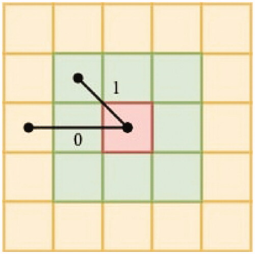
The Graph Convolutional Network (GCN) is a model for mining graph structured data (e.g., social networks, online advertising, etc. Kipf and Welling 2017). In this implementation, we define the map of Africa as an undirected graph, such that the nodes of the graph are the PRIO-GRID cells. Any given cell in the map is immediately connected to its 8 surrounding cells, but is not directly connected to any other cells. This relationship can be referred to as an adjacency matrix defined as A and illustrated in Figure 1 in which the central cell (in red) is connected to a set of adjacent cells (in green), but not directly connected to the rest of the cells (in yellow). The GCN module handles the spatial dependencies by passing the information to each cell from its surrounding cells using a weighted average (convolutions) of their features.

Figure 1. Demonstration of adjacency graph connections. In the adjacency matrix, the edge weights between the red cell and green cells are 1, for a direct connections. The edge weights between the red cell and yellow cells are 0, indicating no direct connection.

Following Kipf and Welling (2017), the spatial dependency model for each time step $t\le P$ has two inputs in this GCN module. The first one is a variable $x_{sp}\in {\mathbb{R}}^{N\times d_0},$ where d₀ is the dimensions of features for each PRIO-GRID cell. The second input is the adjacency matrix A of the graph as in Figure 1. In the adjacency matrix, cells are sorted by acsending order regarding its PRIO-GRID ID. $A_{ij}=1$ means that ith cell is adjacent to jth cell, while $A_{ij}=0$ means that these two cells are not directly connected to each other.

For each time step $t\le P,$ the layer-wise propagation rule of the GCN relationships $H^{(l+1)}$ for layer l of the neural network is: (2) $$H^{(l+1)}=\sigma \left({\tilde{D}}^{-\frac{1}{2}}\tilde{A}{\tilde{D}}^{-\frac{1}{2}}{H}^{(l)}{W}^{(l)}\right),$$(2) where $H^{(l)}\in {\mathbb{R}}^{n\times d}$ is the activation matrix in the lth layer with $H^{(0)}=X.$ With an identity matrix I_N of n dimension, the $\tilde{A}=A+I_N$ is the adjacency matrix of the undirected PRIO-GRID graph $\mathcal{G}$ with self-connections. Here $\tilde{D}$ is the degree matrix which can be represented as ${\tilde{D}}_{ii}=\sum _j{\tilde{A}}_{ij}$ and $W^{(l)}\in {\mathbb{R}}^{d\times d\prime }$ is a layer-specific trainable weight matrix. Here, d and $d\prime$ represent the number of feature dimensions at the lth layer for the input and output, respectively. Finally, $\sigma (·)=\text{ReLU}(·)=\text{max}(0,·)$ is a Rectified Linear Unit (ReLU) activation function that maps across the neural network layers. We choose this because it is an effective activation function in deep learning that allows non-linearity in the neural network.

Equation (2)(2) $$H^{(l+1)}=\sigma \left({\tilde{D}}^{-\frac{1}{2}}\tilde{A}{\tilde{D}}^{-\frac{1}{2}}{H}^{(l)}{W}^{(l)}\right),$$(2) implies a two-step propagation rule for the GCN: (1) aggregate the information from each cell’s neighbors; (2) update the neural network. The ${\tilde{D}}^{-\frac{1}{2}}\tilde{A}{\tilde{D}}^{-\frac{1}{2}}{H}^{(l)}$ term in Equation (2)(2) $$H^{(l+1)}=\sigma \left({\tilde{D}}^{-\frac{1}{2}}\tilde{A}{\tilde{D}}^{-\frac{1}{2}}{H}^{(l)}{W}^{(l)}\right),$$(2) represents the graph convolution, passing the neighbor information to each cell, and then aggregating them based on the connection weights. The aggregating matrix is put into a standard neural network, which multiplies it by the trainable weight matrix $W^{(l)},$ and feeds it to the activation function $\sigma (·).$

Temporal Dependency Modeling

For the temporal aspects of the model, Temporal Convolution Networks (TCN) and Recurrent Neural Networks (RNN) are two main deep learning approaches (Lim and Zohren 2020). Here, we develop temporal models based on both of the spatial and temporal blocks separately. The temporal inputs for each node are $x_{tp}\in {\mathbb{R}}^{P\times d}.$ The TCN is the method selected for temporal modeling, and is the focus of our discussion. The Long Short-Term model (LSTM) is introduced, with details in the Appendix.

The basic idea of TCN-based models is that temporal information is aggregated by learnable convolution filters–similar to moving averages (Yu et al. 2018). Figure 2 shows the basic idea of one dimensional temporal convolution with a kernel of size k. Basically, this operation allows the model to explore the temporal dependency of each node for k months at a time. The convolutional kernel K_t is designed to map the input x_tp to an embedding. In order to keep time steps embeddings consistent along time as P, we pad zero to both beginning and end of the window so it stays the same size.

Figure 2. Demonstration of 1 D convolution. By applying tricks such as padding, we keep the time steps of the outputs the same as inputs. The feature dimension of outputs is determined by the number of filters.

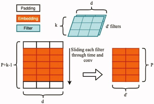
Thus the dimension of embedding after this convolution step is $P\times d\prime .$ Then, an activation function is applied to this embedding and this whole process can be abstracted as: (3) $$H^{(l+1)}=\sigma \left(\text{conv}(H^{(l)},W^{(l)})\right),$$(3) where $\text{conv}$ denotes the convolution operation, and, $W^{(l)}$ is the trainable weight representing the convolutional kernel here with dimension of $k\times d\times d\prime .$

Combined Spatio-Temporal Model

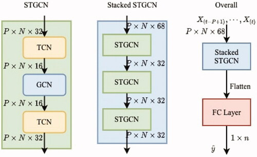
We apply two types of networks to model both the spatial and temporal dependencies. Both TCN and LSTM are explored to model the temporal dependencies. The overall model parameters are shown in Table 1. Similar to last section, we start with the full STGCN-TCN model here and leave the descriptions of STGCN-LSTM to the supplemental materials. Also, we include demonstrations of the basics of STGCN-TCN and STGCN-LSTM models in the supplemental materials.

Table 1. Notations and values of parameters.

Parameter	Values	Meaning
P	54	Number of past steps used for generating predictions
Q	6	Number of future steps for forecasting
d	Variable	Input feature dimension for each instance
$d\prime$	Variable	Output feature dimension for each instance
$S_{\text{tcn}}$	3	Number of stacks for STGCN modules in STGCN-TCN
$S_{\text{lstm}}$	3	Number of stacks for GCN modules in STGCN-LSTM
ktp	3	Kernel size of temporal convolution

Overall, the STGCN-TCN model is composed of stacked modules, and a Fully Connected (FC) layer at the end to generate predictions. We stack three identical STGCN modules altogether to jointly process graph-structured time series. Note it is possible to stack more STGCN modules depending on the requirement of the task and the input dimension for the first STGCN block is different from latter ones as the input features here are the raw data with d = 67.

Figure 3 shows, in each STGCN block, how we stack the sub-modules in TCN-GCN-TCN order. The spatial layer is between the two temporal layers and links those two temporal layers together. Considering the dimensions of both temporal and spatial layers, we purposely design it similar to a “sandwich” structure. This trick is also known as a “bottleneck strategy,” which is very useful when designing a neural network. Having such design encourages the network to compress feature representations to best fit in the available space, to get the best fitting of the loss function during training. Based on existing parameters, each STGCN module is capable of aggregating 1-hop of spatial dependencies, and three months of temporal dependencies. Since the stacked STGCN model has three STGCN modules in it sequentially, overall our proposed framework can aggregate up to 3-hops of spatial dependencies (so 1.5 grid degrees in any direction), and up to 5 months of temporal dependencies. These are tuneable parameters in the model.

Figure 3. Architecture of STGCN-TCN. This framework consists of three STGCN blocks with a fully-connected (FC) layer at the end to generate the forecast outputs.

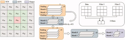
Demonstration of STGCN

Here we demonstrate our proposed model with a simplified example. Suppose that there is an area with 5 × 5 PRIO-GRID cells, for each of the grid cell we have 3 dimensional features, and we have a total of 4 months of data available. Also, we want the model to have the ability of predicting two months ahead. Therefore for the training, we have 2 months of features (X₀ and X₁) and 2 months of labels (y₂ and y₃) available.

We demonstrate the model of STGCN-LSTM in Figure 4. Since there is at most 2-hop connection with respect to the center cell $x_{0a},$ here we apply two layers of GCN module. Each GCN layer can aggregate 1-hop information. Therefore, after the first GCN layer, those surrounding nodes information from $x_{1u}$ where $u\in \{a-h\}$ are encoded into $x_{0a}.$ Nodes such as $x_{1a}$ also aggregate its surrounding information from nodes such as $x_{2a}$ in this first GCN layer. Then, we feed the embedding generated by the 1st layer to the 2nd GCN layer. Since $x_{1u}$ already has $x_{2v},$ where $v\in \{a-p\}$ was encoded from the last layer, then here $x_{0a}$ can theoretically aggregate information from 2-hops away. Next, we feed the embedding generated from the GCN module to LSTM to follow a conventional sequence modeling process. An example of the STGCN-LSTM is shown in Figure 4.

Figure 4. Example of STGCN-LSTM model.

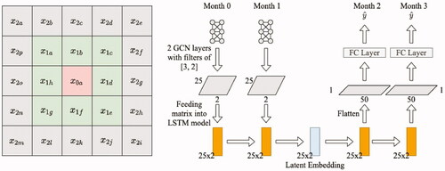
We demonstrate the model of STGCN-TCN in Figure 5. Each module in STGCN-TCN is composed by TCN and GCN structures respectively. Here layers of TCN and GCN models are concatenated together, and extract different types of the information in turn. More specifically, we design the network architecture following a “bottleneck” strategy, which means that dimension of the feature in layers decreases, then increases in this architecture. Notice that in this “sandwich” structure, we have two TCN layers and one GCN layer. Since the filter size in this example is 3, therefore, we can aggregate information up to t – 2 and t + 2 to representations at time t, and consider 1-hop away information using a single TCN-GCN-TCN module.

Figure 5. Example of STGCN-TCN model.

As evidenced by this discussion, neural networks such as the STGCN may have many more parameters than random forest or other machine learning algorithms commonly found in the conflict forecasting literature. To limit the potential for overfitting, we applied three techniques. One, we stacked 3 STGCN-TCN modules to control the overall depth of the frameworks shown in Table 1. Such architecture validates the effectiveness of our proposed framework while keeping the network from becoming “too deep.” Two, we compressed the dimension of embeddings in the neural network, which leads to fewer parameters in the weight matrix. Three, we consider an early stopping mechanism by comparing loss between the training and validation sets.

Model Metrics

For both STGCN-TCN and STGCN-LSTM models, we use mean squared error (MSE) as the training objective function. This objective function represents the average squared differences between predictions for each grid cell of each month to the ground truth. Mathematically, this loss function is defined as: (4) $$L=\frac{1}{QN}\sum _{i=1}^Q\sum _{j=1}^N{\left({\widehat{y}}_j^{(t+i)}-y_j^{(t+i)}\right)}^2.$$(4)

We also consider the continuous rank probability score (CRPS) discussed by Hersbach (2000, 560–1) and Brandt, Freeman, and Schrodt (2014). For a continuous forecast ${\widehat{y}}_j^{(t+i)}$ and an observed value $y_j^{(t+i)}$ suppose we have a pdf for some $\rho (y).$ Then the CRPS is (5) $$\mathit{CRPS}(P,y_j^{t+i})={\int }_{-\infty }^{\infty }{[P({\widehat{y}}_j^{(t+i)})-P_a({\widehat{y}}_j^{(t+i)})]}^2\partial y_j^{t+i}.$$(5)

The CRPS thus compares the cumulative distributions P and P_a where (6) $$P(x)={\int }_{-\infty }^{y_j^{t+i}}\rho (y)dy$$(6) (7) $$P_a(x)=H(x-x_a).$$(7)

Here, H is the Heaviside function: $H(x-x_a)=0$ if $(x-x_a)<0$ and $H(x-x_a)=1$ if $(x-x_a)\ge 0.$ This is an indicator function that compares the total areas of the predicted and observed cumulative distributions, with higher values indicating better alignment of the forecast and observed densities.

The basic difference in the MSE and CRPS is that the MSE is a point metric, which means it scores the model’s prediction but not any uncertainty about that prediction. As a result, if two models make the same point prediction then they have the same MSE. However, one model may have high confidence in that prediction and the other may have low confidence. If the prediction is correct, you would probably expect the model with high confidence to score better than the one with low confidence. As a proper scoring metric, CRPS would score these models differently to account for the distribution of predictions. Brandt, Freeman, and Schrodt (2014) expand on the use of proper scoring metrics like CRPS for conflict forecasting.

Data and Results

Datasets: ViEWS and ICEWS

Our forecasts are based on using (1) the data features of the existing ViEWS baseline random forest model for the log fatalities (Hegre et al. 2019), and (2) augmenting these with event data from ICEWS (Boschee et al. 2015). A total of 18 years of monthly data are used for the results presented here, between January 2000 and December 2016 for training and all of 2017 for validation. The out-of-sample test data are from January 2018 through August 2020. Additional details on the ViEWS forecasting problem can be found in Hegre, Vesco, and Colaresi (2022).

The ViEWS data includes conflict variables such as protest and non-state violence, along with other categories from PRIO-GRID that measure landuse, socioeconomic conditions, natural resources, distances, and accessibility (Tollefsen, Strand, and Buhaug 2012). The full list of features we use can be seen in the Appendix.

In addition to the 48 variables from the ViEWS data, we experiment with ICEWS data (Boschee et al. 2015) retrieved from http://eventdata.utdallas.edu using the UTD Event Data R package (Kim et al. 2019). For each PRIO-GRID cell month, we aggregate the ICEWS event data into counts for each of the 20 CAMEO (2-digit) root codes, as shown in the Appendix (Gerner, Schrodt, and Yilmaz 2009). The ICEWS data are fine-grained and time-variant. Being able to capture changes in the counts of CAMEO root codes over time provides important information that a geographic variable such as elevation would not produce because it is fixed. Our expectation is that this class of highly flexible neural networks can identify patterns in the event data that can improve the predictive performance.

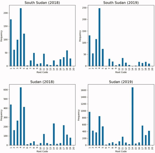
To illustrate the amount of change from one year to the next, Figure 6 shows the total number of instances of each CAMEO root code for South Sudan and Sudan in 2018 and 2019. Overall, South Sudan has experienced a decrease in the total number of events, while Sudan has experienced an increase. South Sudan went from 991 total events in 2018 to 794 total events in 2019. Sudan went from 2,831 total events in 2018 to 6,879 total events in 2019. In South Sudan, we observe a reduction in protest and other forms of conflict including violence (codes 14 and above), while in Sudan we observe increases in these categories. In the case of protest, we observe a drastic increase from 234 to 1,683 protest events.

Figure 6. ICEWS Data for South Sudan and Sudan, 2018 and 2019.

Results

Table 2 shows our primary results. The MSE and CRPS are computed for a rolling 6-months forecast (so six forecasts of each time period) based on the previous 54 months of data for each model. So, the full training period includes data from 2000–2017 and the forecasts roll over January 2018–August 2020 for these computations.

Table 2. Comparisons of results between our proposed methods and baseline methods.

Metrics	RF regressor				STGCN-LSTM (b48-w48)				STGCN-TCN (b32-w60)
Hardware	CPU: i9-7920X				GPU: Quadro RTX 8000
Features	v		v + u		v		v + u		v		v + u
Training Time	∼10 min		∼10 min		∼9 h (50 epochs)		∼9 h (50 epochs)		∼45 min (50 epochs)		∼45 min (50 epochs)
Metrics	MSE	CRPS	MSE	CRPS	MSE	CRPS	MSE	CRPS	MSE	CRPS	MSE	CRPS
Time steps
1	2.86 × 10^–2	9.96 × 10^–3	2.78 × 10^–2	0.13 × 10^–3	2.59 × 10^–2	4.47 × 10^–2	2.37 × 10^–2	1.25 × 10^–2	2.62 × 10^–2	3.25 × 10^–2	2.49 × 10^–2	3.62 × 10^–2
2	2.93 × 10^–2	1.14 × 10^–2	2.85 × 10^–2	1.15 × 10^–2	2.31 × 10^–2	2.25 × 10^–2	2.42 × 10^–2	1.66 × 10^–2	2.43 × 10^–2	3.19 × 10^–2	2.27 × 10^–2	1.65 × 10^–2
3	2.97 × 10^–2	1.20 × 10^–2	2.89 × 10^–2	1.43 × 10^–2	2.59 × 10^–2	4.47 × 10^–2	2.53 × 10^–2	1.32 × 10^–2	2.67 × 10^–2	4.87 × 10^–2	2.26 × 10^–2	3.21 × 10^–2
4	2.96 × 10^–2	1.25 × 10^–2	2.98 × 10^–2	1.19 × 10^–2	3.00 × 10^–2	8.36 × 10^–2	2.55 × 10^–2	3.00 × 10^–2	2.29 × 10^–2	2.73 × 10^–2	2.43 × 10^–2	3.36 × 10^–2
5	2.96 × 10^–2	1.29 × 10^–2	2.92 × 10^–2	1.32 × 10^–2	3.07 × 10^–2	5.60 × 10^–2	2.63 × 10^–2	3.81 × 10^–2	2.26 × 10^–2	8.07 × 10^–3	2.41 × 10^–2	2.65 × 10^–2
6	3.00 × 10^–2	1.29 × 10^–2	2.95 × 10^–2	1.39 × 10^–2	3.07 × 10^–2	7.66 × 10^–2	2.47 × 10^–2	2.26 × 10^–2	2.51 × 10^–2	2.44 × 10^–2	2.30 × 10^–2	2.41 × 10^–2

“v” represents “ViEWS” dataset features and “u” represents “ICEWS/UTD Event Data” features.

We compare our proposed methods (STGCN-LSTM and STGCN-TCN) with the ViEWS benchmark model. We conduct the model comparisons with and without the inclusion of the ICEWS event data, represented by v and v + u respectively so that we can separate the performance of the STGCN model variants from the ICEWS event data.

Figure 7 plots the MSE and CRPS for each model for the six forecast periods. Recall that for MSE/CRPS metrics, smaller/larger values are better when selecting across models and input data. No single model strictly dominates all others. However, using the MSE, the STGCN-TCN offers improvements in predictive performance over the STGCN-LSTM and trains in about 45 minutes compared to nine hours. The STGCN-TCN with the CAMEO event data outperforms the model without (contra, Blair and Sambanis 2020). So, we select the STGCN-TCN model with the ViEWS and ICEWS event data. It is a data-driven, saturated model, and the one we employ for our submitted forecasts for each of the ViEWS tasks (Hegre, Vesco, and Colaresi 2022; Vesco et al. 2022).

Figure 7. Model and data fit comparisons. (a) MSE results. (b) CRPS results.

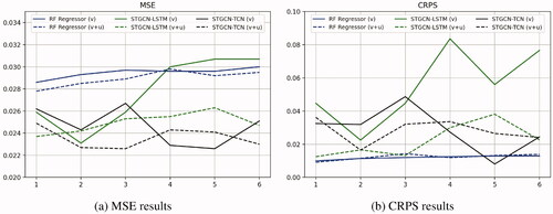
Alternatively, panel (b) of Figure 7 shows that when we use a proper forecast scoring rule as suggested by Brandt, Freeman, and Schrodt (2014), the model and variable selection rankings are different. While there is clear evidence of the value of the STGCN models over the benchmark, there is mixed evidence about the two STGCN models and the event data contributions. Overall, the STGCN-LSTM without the event data performs best, and for each forecast period it performs better than the STGCN-LSTM with event data.

To further assess the potential contribution of the ICEWS variables for the ViEWS forecasting problem, we compared the MSE contributions of different sets of variables using a stepwise elimination approach similar to Ward, Greenhill, and Bakke (2010). We grouped the variables into six categories, most of which are based on Tollefsen, Strand, and Buhaug (2015): violence and instability (G1), landuse (G2), socioeconomic (G3), resource (G4), distance, area, and accessibility (G5), and CAMEO (G6). The variables in each category can be seen in the Appendix.

Figure 8 shows the marginal contributions for each group. The steps proceed in a backwards elimination fashion. At each step, we remove each feature group, one at a time, and calculate the MSE after retraining with the remaining features. We do this for each forecasting length, 1 through 6, and take the average MSE. The group with the largest increase in MSE is the one with the greatest contribution at that step. This group is then removed and we repeat the process for the next step.

Figure 8. Marginal contributions plot for each group of covariates.

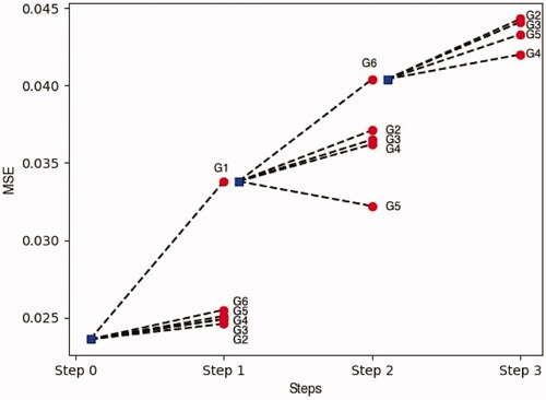
The three most important feature groups are G1, G6, and G2. G1 is our violence and instability group and contributes the most to our forecasts. This is consistent with findings reported in Vesco et al. (2022) and D’Orazio and Lin (2022) for this forecasting window. After eliminating the conflict features in Step 1, the CAMEO variables (G6) have the largest contribution in Step 2. This suggests that these time-variant event measures contribute more than the other slow-moving or invariant indicators, at least when using the MSE which is one of the main ViEWS scoring metrics (Hegre, Vesco, and Colaresi 2022; Vesco et al. 2022).

Additional results for ViEWS Task 2 and Task 3 are shown in the Appendix.

Exploration

Using the STGCN-TCN with the ICEWS event data, we produced true, a priori forecasts for each month from October 2020 through March 2021 (ViEWS Task 1). The level of forecasted fatalities for October and March is shown in Figure 9, and the forecasted change in fatalities is shown in Figure 10.

Figure 9. Real predictions for Oct. 2020 and Mar. 2021.

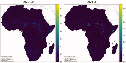
Figure 10. Delta predictions for Oct. 2020 and Mar. 2021.

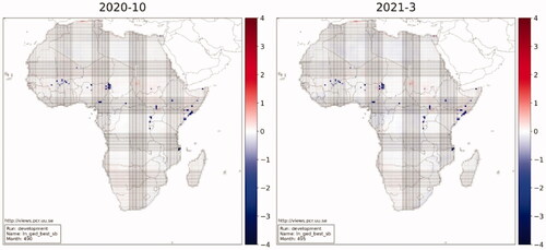
Looking at Figure 9, violence is expected to occur primarily in four regions: Nigeria’s Borno State and other areas near Lake Chad; South Sudan and the southern area of Sudan; the southern regions of Somalia including border areas with Kenya and Ethiopia; and the DRC’s eastern border with Uganda, Rwanda, and Burundi between Lakes Albert and Tanganyika. As we can see in Figure 10, violence in Sudan is expected to get worse, as there are many grids shaded red and only a few that are blue. In the other three areas, there are several grids shaded darker blue, which implies larger expected reductions.

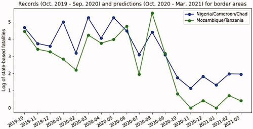
Another area of interest is the border of Mozambique and Tanzania. Violence has intensified in this region recently (Campbell 2020; Blake 2020). Our model forecasts reductions here, as it does not predict instances of state-based violence. It is worth noting that there is a distinction in state-based violence and non-state violence, and our model offers no forecasts on the latter.

Observed and predicted violence for the Mozambique-Tanzania border area, and the Lake Chad region, are shown in Figure 11. To create this plot, we used the natural log of the sum total of state-based fatalities for all grids in each region. In both instances, the observed violence, which spans October 2019 through September 2020, is relatively high. Forecasted violence, which is shown from October 2020 through March 2021, is considerably lower.

Figure 11. Records and predictions for border areas.

Across Africa, our model forecasts decreases in violence in 3,690 grids and increases in violence in 6,987 grids for October 2020. However, the largest expected increase is 0.705, while the largest expected decrease is 5.12. A similar pattern holds for all months from October through March, in that the largest forecasted increase is a smaller number (maximum is 0.862) while the largest expected decrease is a larger number (maximum is 5.19). However, the ratio of forecasted decreases-to-increases changes. For October the ratio is about 0.53:1, and for March it is flipped to about 1.71:1.

Conclusion

We explored three different model components to improve predictive performance over the ViEWS benchmark: a class of neural network that accounts for spatial and temporal dependencies, the use of CAMEO-coded event data, and the CRPS which is a proper scoring metric. Our experiments show that, when using MSE as performance metric, the best performing model is the STGCN-TCN with event data measures. If we were to use the CRPS for model selection, the results would not be entirely consistent with that of MSE.

Each of these areas–algorithms, measures, and metrics–provide opportunities for future research to improve our understanding of patterns of violence. By analyzing the dynamics of violence at the grid-month level in Africa, our results consistently show that neural networks taking into consideration spatial and temporal dependencies offer improvements over more traditional machine learning methods. Our model can be further improved in three directions: model complexity, hyperparameters, and interpretability.

Model complexity: Most existing frameworks are based on a two-step protocol: first, apply Graph Convolutional Networks (GCN) module to extract the spatial dependencies out of the graph structured data; then, incorporate a Recurrent Neural Network (RNN) module (Li et al. 2018) or a Convolutional Neural Network (CNN) module to model the temporal dependencies (Wu et al. 2019). Even though this two-step paradigm typically goes unquestioned, Lea et al. (2016) argue that the model suffers from the loss of valuable information between steps. Also, for temporal dependency modeling, CNN-based methods normally require multiple 1 D convolution layers to properly learn temporal information from long sequences, which could lead to a very deep neural network structure. Therefore, a possible solution is to design a unified spatio-temporal graph neural network for time series forecasting. The key idea is that if we can construct an appropriate graph over sequences of data, including both spatial and temporal information, then a single graph neural network could be trained to capture both dependencies simultaneously. Such a model could reduce the types of neural network structure in the solution from two to one, which could dramatically decrease the complexity of model.

Hyperparameters: Tuning parameters for neural networks can be complicated, especially when the model is very deep. These models require a lot of computational resource, leading to very long training times. Therefore, trying all hyperparameter combinations is normally not possible. In this paper, we initially set hyperparameters like learning rate, batch size, and the dimension of the GCN using values from similar models in other applications. Then, we prepare candidate sets for these hyperparameters surrounding the initial settings, and conducted grid search for the best among candidates. However, we were unable to cover a very large portion of the search space due to the complex structure of the model. Recently, some researchers argue that by combining grid search with Bayesian Optimization algorithms, it is possible to get the optimal parameters in a relatively shorter period (Frazier 2018). The key idea of using Bayesian Optimization on the hyperparameters is that the prior knowledge of model performance could imply the posterior probability of best settings, which basically provides line of sight about which directions to adjust those hyperparameters.

Interpretability: Normally neural networks are considered to be a black-box model due to their nonlinear nature induced by deep networks structures. This observation also applies to our model. However, for political science studies, reserving the interpretability at a certain level is appreciated when accurate forecasts are made, since reasoning is really important during the policymaking process. During our experiment, we met difficulties, mainly regarding computation time, when applying state-of-the-art deep learning interpretable models, such as SHAP. We plan to further investigate potential solutions to address this problem.

Event data continue to offer promise in the field of conflict forecasting, as they are a prime source of fine-grained, time-variant measures. While ICEWS offers high-quality event data coded using automated, dictionary-based methdos, there are new techniques emerging in the field of natural language processing that appear promising. Specifically, transformer models may be able to improve the validity of event data substantially, reducing noise and improving performance of models that incorporate event measures (Parolin et al. 2020).

The application of proper scoring metrics like the CRPS is not new to the ViEWS team, as the TADDA measure is itself a proper scoring metric. As our results show, and as the differences in MSE and TADDA show in the evaluation (Hegre, Vesco, and Colaresi 2022; Vesco et al. 2022), choice of metric matters as different models perform differently based on which measure is chosen. Importantly, there is no inherently “correct” performance measure. While researchers should be mindful of the differences, they should also try to align the selection of performance metric with the end-goal of the model. If the model is intended to be used by analysts in government, for example, then the analysts should decide on the performance measure that best matches their goals for the model. MSE is simple to understand, and thus is a useful generic metric for communicating results. But as our application of CRPS and the ViEWS’ TADDA measure (Hegre, Vesco, and Colaresi 2022) show, the selected model is not always consistent with other measures.

Acknowledgements

We would like to thank Mike Colaresi, Håvard Hegre, and Paola Vesco for their work organizing the Violence Early Warning System prediction competition and workshop. We would also like to thank the competition scoring committee, Nils Weidmann, Adeline Lo, and Gregor Reisch, and all competition and workshop participants.

Data availability statement

Replication materials are available at http://dvn.iq.harvard.edu/dvn/dv/internationalinteractions. All questions regarding replication may be directed to Yi-Fan Li.

Correction Statement

This article was originally published with errors, which have now been corrected in the online version. Please see Correction (http://dx.doi.org/10.1080/03050629.2022.2101217).

Additional information

Funding

This material is based upon work supported by the National Science Foundation under Grant Numbers [DMS 1737978 and OAC 1931541]. Any opinions, findings, and conclusions or recommendations expressed in this material are those of the author(s) and do not necessarily reflect the views of the National Science Foundation.

References

- Beck, N., G. King, and L. Zeng. 2000. “Improving Quantitative Studies of International Conflict: A Conjecture.” American Political Science Review 94 (1): 21–35. doi:10.1017/S0003055400220078.
- Berman, N., M. Couttenier, D. Rohner, and M. Thoenig. 2017. “This Mine Is Mine! How Minerals Fuel Conflicts in Africa.” American Economic Review 107 (6): 1564–1610. doi:10.1257/aer.20150774.
- Binkowski, M., G. Marti, and P. Donnat. 2018. “Autoregressive Convolutional Neural Networks for Asynchronous Time Series.” In Vol. 80 of the Proceedings of the International Conference on Machine Learning, edited by Jennifer Dy and Andreas Krause, 580–589. Stockholm: PMLR.
- Blair, R. A., and N. Sambanis. 2020. “Forecasting Civil Wars: Theory and Structure in an Age of ‘Big Data’ and Machine Learning.” Journal of Conflict Resolution 64 (10): 1885–1915. doi:10.1177/0022002720918923.
- Blake, J. 2020. “Preventing the Next Boko Haram in Northern Mozambique.” Council on Foreign Relations, May 20. Accessed 14 December 2020. https://www.cfr.org/blog/preventingnext-boko-haram-northern-mozambique
- Boschee, E., J. Lautenschlager, S. O’Brien, S. Shellman, J. Starz, and M. Ward. 2015. “ICEWS” Coded Event Data.” Harvard Dataverse V30. Accessed 20 February 2022. doi:10.7910/DVN/28075.
- Brandt, P. T., J. R. Freeman, and P. A. Schrodt. 2014. “Evaluating Forecasts of Political Conflict Dynamics.” International Journal of Forecasting 30 (4): 944–962. doi:10.1016/j.ijforecast.2014.03.014.
- Buhaug, H., and K. S. Gleditsch. 2008. “Contagion or Confusion? Why Conflicts Cluster in Space.” International Studies Quarterly 52 (2): 215–233. doi:10.1111/j.1468-2478.2008.00499.x.
- Campbell, J. 2020. “The Military-First Approach in Northern Mozambique Is Bound to Fail.” Accessed 14 December 2020. https://www.cfr.org/blog/military-first-approach-northern-mozambique-bound-fail.
- Chiba, D., and K. S. Gleditsch. 2017. “The Shape of Things to Come? Expanding the Inequality and Grievance Model for Civil War Forecasts with Event Data.” Journal of Peace Research 54 (2): 275–297. doi:10.1177/0022343316684192.
- Cranmer, S. J., and B. A. Desmarais. 2017. “What Can We Learn from Predictive Modeling?” Political Analysis 25 (2): 145–166. doi:10.1017/pan.2017.3.
- Deng, L., and Y. Liu. 2018. Deep Learning in Natural Language Processing. New York: Springer.
- D’Orazio, V. 2020. “Conflict Forecasting and Prediction.” Oxford Research Encyclopedia of International Studies. doi:10.1093/acrefore/9780190846626.013.514.
- D’Orazio, V., and Y. Lin. 2022. “Forecasting Conflict in Africa with Automated Machine Learning Systems.” International Interactions 48 (4). doi:10.1080/03050629.2022.2017290
- Dorff, C., M. Gallop, and S. Minhas. 2020. “Networks of Violence: Predicting Conflict in N”Igeria.” The Journal of Politics 82 (2): 476–493. doi:10.1086/706459.
- Findley, M. G., and J. K. Young. 2012. “Terrorism and Civil War: A Spatial and Temporal Approach to a Conceptual Problem.” Perspectives on Politics 10 (2): 285–305. doi:10.1017/S1537592712000679.
- Frazier, P. I. 2018. “A Tutorial on Bayesian Optimization.” arXiv preprint arXiv:1807.02811.
- Gerner, D. J., P. A. Schrodt, and Ö. Yilmaz. 2009. “Conflict and Mediation Event Observations (CAMEO): An Event Data Framework for a Post Cold War World.” In International Conflict Mediation: New Approaches and Findings, edited by J. Bercovitch and S. Gartner, 287–304. New York: Routledge.
- Guo, S., Y. Lin, N. Feng, C. Song, and H. Wan. 2019. “Attention Based Spatial-Temporal Graph Convolutional Networks for Traffic Flow Forecasting.” I Vol. 33 of the Proceedings of the AAAI Conference on Artificial Intelligence, 922–929. Palo Alto: AAAI Press.
- Hegre, H., C. Bell, M. Colaresi, M. Croicu, F. Hoyles, R. Jansen, M. R. Leis, et al. 2021. “ViEWS2020: Revising and Evaluating the ViEWS Political Violence Early-Warning System.” Journal of Peace Research 58 (3): 599–611. doi:10.1177/0022343320962157.
- Hegre, H., M. Allansson, M. Basedau, M. Colaresi, M. Croicu, H. Fjelde, F. Hoyles, et al. 2019. ‘ViEWS’: A Political Violence Early-Warning System.” Journal of Peace Research 56 (2): 155–174. doi:10.1177/0022343319823860.
- Hegre, Håvard, Paola Vesco, and Michael Colaresi. 2022. “Lessons from an Escalation Prediction Competition.” International Interactions. 48 (4).
- Hersbach, H. 2000. “Decomposition of the Continuous Ranked Probability Score for Ensemble Prediction Systems.” Weather and Forecasting 15 (5): 559–570. doi:10.1175/1520-0434(2000)015<0559:DOTCRP>2.0.CO;2.
- Hill, D. W., and Z. M. Jones. 2014. “An Empirical Evaluation of Explanations for State Repression.” American Political Science Review 108 (3): 661–687. doi:10.1017/S0003055414000306.
- Kane, M. J., N. Price, M. Scotch, and P. Rabinowitz. 2014. “Comparison of ARIMA and Random Forest Time Series Models for Prediction of Avian Influenza H5N1 Outbreaks.” BMC Bioinformatics 15 (1): 1–9. doi:10.1186/1471-2105-15-276.
- Kim, H., V. D’Orazio, P. T. Brandt, J. Looper, S. Salam, L. Khan, and M. Shoemate. 2019. “UTD”Eventdata: An R Package to Access Political Event Data.” Journal of Open Source Software 4 (36): 1322. doi:10.21105/joss.01322.
- Kipf, T. N., and M. Welling. 2017. “Semi-Supervised Classification with Graph Convolutional Networks.” Paper presented at the 5th International Conference on Learning Representations, ICLR 2017, Toulon, April 24–26.
- Lea C., Vidal R., Reiter A., Hager G.D. 2016. “Temporal Convolutional Networks: A Unified Approach to Action Segmentation.” In: Computer Vision – ECCV 2016 Workshops, edited by G. Hu, and H. Jégou. ECCV 2016. Cham: Springer.
- Li, Y., K. Fu, Z. Wang, C. Shahabi, J. Ye, and Y. Liu. 2018. “Multi-Task Representation Learning for Travel Time Estimation.” Paper presented at the Proceedings of the 24th ACM SIGKDD International Conference on Knowledge Discovery & Data Mining, London, August 19-23.
- Li, Y., R. Yu, C. Shahabi, and Y. Liu. 2018. “Diffusion Convolutional Recurrent Neural Network: Data-Driven Traffic Forecasting.” International Conference on Learning Representations.
- Lim, B., and S. Zohren. 2020. “Time Series Forecasting With Deep Learning: A Survey.” arXiv preprint arXiv:2004.13408.
- McClelland, C. A. 1976. “World Event/Interaction Survey Codebook (ICPSR 5211).”
- Parolin, E. S., L. Khan, J. Osorio, V. D’Orazio, P. T. Brandt, and J. Holmes. 2020. “HANKE: Hierarchical Attention Networks for Knowledge Extraction in Political Science Domain.” Paper presented at the 2020 IEEE 7th International Conference on Data Science and Advanced Analytics (DSAA), Sydney, October 6-9.
- Schrodt, P. A. 2012. “Precedents, Progress, and Prospects in Political Event Data.” International Interactions 38 (4): 546–569. doi:10.1080/03050629.2012.697430.
- Seo, Y., M. Defferrard, P. Vandergheynst, and X. Bresson. 2018. “Structured Sequence Modeling with Graph Convolutional Recurrent Networks.” International Conference on Neural Information Processing, 362–373. Springer.
- Siami-Namini, S., N. Tavakoli, and A. S. Namin. 2018. “A Comparison of ARIMA and LSTM in Forecasting Time Series.” 2018 17th IEEE International Conference on Machine Learning and Applications (ICMLA), 1394–1401. IEEE. doi:10.1109/ICMLA.2018.00227.
- Tollefsen, A. F., H. Strand, and H. Buhaug. 2012. “PRIO-GRID: A Unified Spatial Data Structure.” Journal of Peace Research 49 (2): 363–374. doi:10.1177/0022343311431287.
- Tollefsen, A. F., K. Bahgat, J. Nordkvelle, and H. Buhaug. 2015. “PRIO-GRID v.2.0 Codebook.”
- Vesco, Paola, H. Hegre, M. Colaresi, B. J. Remco, A. Lo, G. Reisch, and N. Weidmann. 2022. “United They Stand: Findings from an Escalation Prediction Competition.” International Interactions 48 (4). doi:10.1080/03050629.2022.2029856
- Wang, X., Y. Ma, Y. Wang, W. Jin, X. Wang, J. Tang, C. Jia, and J. Yu. 2020. “Traffic Flow Prediction via Spatial Temporal Graph Neural Network.” Proceedings of the Web Conference 2020, 1082–1092.
- Ward, M. D., B. D. Greenhill, and K. M. Bakke. 2010. “The Perils of Policy by p-Value: Predicting Civil Conflicts.” Journal of Peace Research 47 (4): 363–375. doi:10.1177/0022343309356491.
- Wu, Z., S. Pan, G. Long, J. Jiang, and C. Zhang. 2019. “Graph Wavenet for Deep Spatial-Temporal Graph Modeling.” Proceedings of the 28th International Joint Conference on Artificial Intelligence, 1907–1913. AAAI Press.
- Yan, S., Y. Xiong, and D. Lin. 2018. “Spatial Temporal Graph Convolutional Networks for Skeleton-Based Action Recognition.” arXiv preprint arXiv:1801.07455.
- Yu, B., H. Yin, and Z. Zhu. 2018. “Spatio-Temporal Graph Convolutional Networks: A Deep Learning Framework for Traffic Forecasting.” In Proceedings of the Twenty-Seventh International Joint Conference on Artificial Intelligence, IJCAI 2018, July 13-19, 2018, Stockholm, Sweden, edited by J. Lang, 3634–3640. ijcai.org.
- Zhang, J., X. Shi, J. Xie, H. Ma, I. King, and D.-Y. Yeung. 2018. “Gaan: Gated Attention Networks for Learning on Large and Spatiotemporal Graphs.” arXiv preprint arXiv:1803.07294.