Time-consistent and market-consistent actuarial valuation of the participating pension contract

Abstract

The regulator in Europe calls for the market-consistent valuation of the insurance liabilities that usually are not (fully) tradable. An example of such liabilities is the participating pension contract that is generally long-dated and vulnerable to the medium-time dynamics of the underlying risk drivers. Dealing with these characteristics requires time-consistent pricing. However, the well-known non-linear premium principles, often used as pricing operators, are not time-consistent. Based on this motivation, we study the time-consistent and market- consistent (TCMC) actuarial valuation of the participating pension contracts with hybrid payoff. We use a standard profit-sharing mechanism with guaranteed interest rate, and generalize it to a hybrid profit-sharing mechanism with the actuarial and hedgeable financial risks, over the course of the contract. Market-consistency is maintained by “two-step actuarial valuation” in a one-period setting. Time-consistency is obtained by a “backward iteration” of these one-period two-step valuations over the predetermined sub-intervals of the valuation period. We use the Least-Square Monte-Carlo method to implement the conditional operators in the backward iteration. We compare the results of TCMC price to the expected value of the discounted payoff and measure the relative risk loading and time-consistency risk premium. Besides, we investigate the effect of the stochastic interest rate as compared to the deterministic one.

Keywords:

• Market-consistent
• time-consistent
• actuarial price
• participating pension contract
• two-step valuation
• backward-iteration
• hybrid payoff
• profit-sharing

1. Introduction

Pension contract valuation is significantly related to the different risk factors involved in the assets and liabilities of a pension fund or insurance company. Simply put, the money collected by the pension fund from policyholders is typically invested in different financial markets such as equities, bonds, and properties like real states and form the asset side of the balance sheet. On the liability side, the main factor is the reserves to compensate for the future benefits to policyholders, apart from the bonus reserve or the buffer of the fund. The value of the pension policy and its payoff predominantly depends on the return on the asset side and the liabilities to assets ratio.

Concerning the assets invested in equities, some of the main risk factors that would affect the pension fund are volatility, interest rate risk, and market risks. The fund is also exposed to credit risk via investments in bonds that may default, and to liquidity risk on assets such as real estate and other properties. On the liability side, the longevity risk related to the future life of the policyholders plays the main role. Moreover, economic factors such as inflation and wage growth directly affect liabilities and can indirectly affect investment assets.

The payoffs of most modern forms of life insurance and pension contracts, such as participating policies, annuities, unit-linked plans, and pension schemes, are a mixture of the above-mentioned risk factors that are stochastic and can be classified into two main categories: financial and actuarial risks. In this study, the only financial risk we consider is the equity risk with constant volatility and stochastic interest rate, and the only actuarial risk we consider is mortality/longevity risk.

Pension liabilities are not commonly traded in the market and are, therefore (partially) un-hedgeable. Nevertheless, in recent years, regulators have started to recommend the assessment of the market value of the liabilities to insurance companies and pension funds, even though there is no liquid market for them.¹ Since there is an underlying unhedgeable actuarial risk (mortality/longevity) in pension contracts, we consider the actuarial value of the contract instead of the arbitrage-free assumption in the pricing method. However, on the other hand, the financial risk drivers in the contract payoff must be addressed through a financial pricing framework. After all, if there is any correlation between actuarial and financial risks, the price must reflect the possible partial hedging for the actuarial risk through financial market dynamics. This is ensured by the market-consistency condition of the pricing operator. Some researchers consider the above conditions in the explicit definition of market-consistency for pricing operators. See for example, Pelsser & Stadje (2014), Kupper et al. (2008), and Malamud et al. (2008).

On the other hand, pension contracts impose very long-dated liabilities on the issuer. In most cases, people start their policy at age 20–25 years and are expected to live until age 70–85 years, with the oldest living individuals being around 110–115 years of age. During such a long period, pension liabilities are affected by substantial social, economic, and financial shocks. If we focus on the effect of financial and actuarial risks over such a long-term valuation period, the price of the pension contract should capture and reflect market dynamics in the medium-term on the liability value. For example, when the contract includes the bonus or surrounding option, under market-consistency, the contract should be re-valuated to incorporate the market-risk factors in the medium term. To reflect such re-valuation over the valuation period, the price must be ‘time-consistent’. Time-consistency implies that if the pension liability position $\left(A\right)$ is more expensive than position $\left(B\right)$ at a (long-dated) maturity, it is then also more expensive at any time prior to that point. Hence, to obtain time-consistency, ‘dynamic’ valuation should be used to price the pension contract. For discussions on time-consistency and its connection to dynamic risk measures, we refer to Cheridito et al. (2006), Roorda et al. (2005), Rosazza Gianin (2006), Cheridito & Stadje (2009), Artzner et al. (2007), Acciaio & Penner (2011), Cheridito & Kupper (2011), Follmer & Penner (2006), and Penner (2007).

Several researchers have attempted to model the value of the contract with different underlying risk factors. Grosen & Jorgensen (2000) valuated a participating pension contract with surrounding options using a stochastic return on investment asset in a Black-Scholes economy with a constant interest rate and a guaranteed return in valuation. Zaglauer & Bauer (2008) develop the model by adding a stochastic interest rate and uses the Monte Carlo method to value the contract. They realize that the embedded options in the contract are considerably sensitive to making the constant interest rate stochastic. Bernard et al. (2005) extend a similar model by incorporating the default risk of the issuer and use the least Square Monte Carlo (LSMC) method for valuation. Tanskanen & Lukkarinen (2003) provide the fair value of a contract with more flexibility on the bonus policy in the model. For more on valuation of the participating policies, see Kleinow (2009) and Bacinello (2003). The majority of the above-mentioned literature considers pricing contracts in an arbitrage-free condition, which implicitly assumes a liquid market for liabilities, even though such a market does not exist.

We focus on the valuation of the participating pension policy (PPP). Normally, a participating policy is characterized by a guaranteed annual return plus bonus option, which can be distributed under a special mechanism related to the ratio of assets and liabilities. Moreover, most of the participating policies offer a surrounding option to sell the policy back to the pension fund or insurance company and receive the surrounding value.

We calculate the actuarial price of the participating policy under time-consistency and market-consistency arguments. To achieve market-consistency for a conditional pricing operator, such as actuarial premium principles, Pelsser & Stadje (2014) introduce the theoretical framework of ‘Two-step market evaluation’. This framework can be used for any hybrid payoff with underlying financial and actuarial risks. A similar method is used by Møller (2002) to achieve market-consistency for the Standard-Deviation actuarial principle and by Musiela & Zariphopoulou (2004) for indifference premium via exponential utility function in an incomplete market.

To implement a time-consistent risk measure, Jobert & Rogers (2008) show that time-consistency can be achieved for a price operator by backward iteration of one-period static operators starting from maturity and going back over the longer valuation period. Stadje (2010) obtain the continuous-time limit of the dynamic convex risk measures by taking the limit over the same discrete-time risk measures. Finally, Salahnejhad & Pelsser (2016) use the backward iteration method to obtain the continuous-time limit of the time-consistent actuarial premium principles, when the underlying actuarial risk is modeled with diffusion and jump-diffusion stochastic processes.

Pelsser & Stadje (2014) also show that market-consistency obtained by the two-step market evaluation holds in a dynamic setting under time-consistency. Moreover, they prove that market-consistency is preserved and valid for a finite number of points over the pricing period, where the pricing operator is time-consistent. Later, Salahnejhad & Pelsser (2020) introduce an applied framework for the two-step actuarial operators and its application to calculate EIOPA risk-margin method. They applied backward iteration to the two-step operators to deliver a combined time-consistent and market-consistent actuarial premium for a simplified unit-linked contract. Some new developments on the market-consistent valuation can be found in Dhaene et al. (2017) where a one-period framework of ‘Fair valuation’ is a hedge-based method and both market-consistent and actuarial. Then, the two papers Delong et al. (2019a, 2019b) extends the the one-period setting into multi-period using the similar backward iteration method. For further studies the readers can see Deelstra et al. (2019), Barigou & Dhaene (2019), Barigou et al. (2019) and Chen et al. (2020).

We assume that the hybrid payoff is a combination of the investment on equity, interest rate, and the mortality/longevity risks; for simplicity, we assume that volatility is constant. Under the two-step actuarial valuation, financial risks must be priced under the assumption of market completeness and no-arbitrage conditions. We model the investment asset in a Black & Scholes (1973) framework with a Geometric Brownian motion (GBM) where there exists a unique martingale measure $\mathbb{Q}$ equivalent to the real-world measure $\mathbb{P}$, under which the price is a conditional expectation of the discounted payoff. Due to flexibility and adaptability to discretization schemes, among a wide variety of models, we choose the Hull & White (1996) short rate model for the interest rate risk. Regarding mortality/longevity risk, Lee & Carter (1992) study mortality trends with a time specified stochastic index and combine it with age-specified average trend and sensitivity coefficient to formulate the projected force of mortality. The Lee–Carter model is used a lot in applications as a discrete-time (normally annual) model. Among other extensions, Renshaw & Haberman (2006) extend the Lee–Carter model by adding a cohort-based factor to the model. On the other hand, Cairns et al. (2006) model stochastic mortality in a continuous-time setting similar to the model of positive interest rate risk. They use the model to price mortality-indexed products under the no-arbitrage condition. Cairns et al. (2009, 2011) later compare different stochastic mortality models and their results on mortality data of different countries. As we consider a discrete-time framework, and because it is widely used in the industry, we use the Lee–Carter model. All risk drivers are assumed to follow a diffusion process.

To numerically calculate the price of the contract, we focus on the finite-difference intervals as the main setup for the discretization of the underlying process and specify the payoff functions accordingly. To choose the most feasible numerical approach, we consider the fact that the bonus and interest crediting mechanism in participating policy results in a path-dependent process for the policy reserve.² On the other hand, the backward iteration of the conditional one-period price operator over the long-term valuation period imposes a huge load on the calculation. In particular, the higher dimension of the underlying risk drivers makes the situation worse and leads to exploding calculations of this dynamic valuation. To generate more speed and efficiency, Carriere (1996) and Longstaff & Schwartz (2001) introduce a method called Least Square Monte Carlo (LSMC) to price American options. The method is widely used and developed as an efficient numerical method in theory and application. For a well-known reference on LSMC see the book by Glasserman (2004) and papers by Glasserman & Yu (2004a, 2004b). As regards life and pension liabilities, see Angelis et al. (2014) for the usage of the lattice method to discretize the investment asset and interest rate in participating policies, and Bacinello et al. (2011) for valuation of variable annuities with LSMC. For the application of LSMC to value the participating contract and its surrounding options, see Bacinello et al. (2010), Li & Szimayer (2014), and Létourneau & Stentoft (2014).

The rest of the paper is structured as follows: We start in Section 2 by introducing the participating contract and models for the underlying risk drivers. Then, we explain the liability dynamics and define the new hybrid crediting mechanism that is built based on the Grosen-Jorgensen framework, which forms the hybrid policy reserve in the final payoff. We conclude this section by providing the dynamics of the survival probability and the technical profit-sharing component in the hybrid crediting mechanism under the Lee–Carter model. In Section 3, we explain the pricing framework by introducing the two-step actuarial operator and executing the backward-iteration of the one-period valuation on the two-step operator. The method achieves a time-consistent price. Section 4 discusses the suggested numerical method to implement the pricing framework. The first part of this section is about simulating the hybrid policy reserve and the crediting interest rate. Then, we explain the regression-based method and adopt a version of this method that corresponds to the needed quantities in the hybrid profit-sharing mechanism of the participating contract. Finally, we formulate the calculation of the time-consistent two-step Standard-deviation price by using the regression-based method. In Section 5, we provide the results of the numerical procedure to price the participating contract. In the first subsection, we deliver the time-consistent and market-consistent price and compare it with the expected value price and the one-period market-consistent price. We then examine the sensitivity of the price to the volatility of the investment asset, the parameters of the funding policy, and the randomness of the interest rate risk. Section 6 summarizes the paper and presents the conclusion.

2. Model and setup

The ‘participating policy’ (i.e. with profit) is a practical, familiar form of pension contracts that has most of the main attributes of pension policies. These attributes include periodical crediting of a policy interest with a guaranteed rate, which is the link of the policy to the financial market.

We choose a well-structured version of the participating policy proposed by Grosen & Jorgensen (2000). According to the payoff and crediting mechanism, the policy is, by construction, linked to the Dutch pension payoff. In the Grosen & Jorgensen (2000) setting, the payoff is considered. At time t = 0, a cohort of the policyholders buy one unit of the contract with nominal value $P_0$ for a single price $V_0$. The insurance company invests all its money in the financial market, and at the end of every year t, is committed to credit policy interest rate $r_P\left(t\right)$ that cannot be less than a guaranteed rate $r_G$. At the time of maturity T, the policy ends by paying a single value $P_T$ to each policyholder. However, in the real world, apart from financial factors, the longevity risk affects the evolution and maturity of the policy reserve on the liability side through the number of survivors. To address this, we explain the liability dynamics and evolution of the policy reserve under the Grosen & Jorgensen (2000) setting in Subsection 2.2. Then we modify the setting to a hybrid financial and actuarial dynamic by incorporating the number of survivors $N_x\left(t\right)$ at time t to form the policy reserve and the payoff, regarding the starting cohort $N_x\left(0\right)$.

As the main focus of this study is implementing a market-consistent framework to price the participating pension contract, we skip the surrender option for the sake of simplicity. Later, in the numerical phase in Section 5, we calculate the price in two different situations where the risk-free interest rate is constant and stochastic. Thus, we analyze the effect of stochastic interest rate on the price of the contract.

2.1. Risk drivers

The three main underlying risk drivers present in the pension policy will be modeled as follows:

• Mortality/longevity (Lee–Carter): We model the mortality/longevity risk with the forecasting mortality Lee–Carter model. For an integer age x in calendar year t, the Lee–Carter model assumes the following dynamics for the force-of-mortality ${\mu }_x\left(t\right)$ (1) $\ln {\mu }_x\left(t\right)={\alpha }_x+{\text{β}}_x{\kappa }_t$(1) that makes ${\mu }_x\left(t\right)$ a stochastic function with the underlying process $\kappa \left(t\right)$, which follows a Brownian motion with drift as (2) $\mathrm{d}{\kappa }_t={\mu }_{\kappa }\mathrm{d}t+{\sigma }_{\kappa }\mathrm{d}{W}_t^{\kappa }.$(2) where $W_t^{\kappa }$ is the standard Brownian motion under the real-world probability measure $\mathbb{P}$, and ${\mu }_{\kappa }$ and ${\sigma }_{\kappa }$ are constant. In the Lee–Carter model, ${\kappa }_t$ is the latent process to model the longevity trend over time, ${\alpha }_x$ is the average age-specific mortality, and ${\text{β}}_x$ is the age-specific sensitivity of the mortality to a change in ${\kappa }_t$.

  Although applications of the model only use a discrete setting with a constant parameter over each year, the model can theoretically apply to continuous-time dynamics.

• Investment Asset (Black-Scholes): We model the investment asset at time t, $A_t$, by a two-factor Geometric Brownian Motion (GBM) (3) $\mathrm{d}{A}_t={\mu }_A{A}_t\mathrm{d}t+{\sigma }_A{A}_t\mathrm{d}{\tilde{W}}_t^A.$(3) where ${\mu }_t^A$ is the stochastic growth rate, ${\sigma }_A$ is the constant volatility, and $W_t^A$ is a standard Brownian motion under the real-world measure $\mathbb{P}$. As we assume that the financial market is complete and arbitrage-free, there exists a unique equivalent martingale measure $\mathbb{Q}$ according to the second fundamental theorem of asset pricing, for which $A_t$ follows the risk-adjusted GBM below (4) $\mathrm{d}{A}_t=r_t{A}_t\mathrm{d}t+{\sigma }_A{A}_t\mathrm{d}{W}_t^A.$(4) with the solution (5) $A_t=A_0\exp \left(\left(r_t-\frac{1}{2}{\sigma }_A^2\right)t+{\sigma }_A{W}_t^A\right),$(5) where $A_0$ is the initial value of the investment, $W_t^A$ is standard Brownian motion under $\mathbb{Q}$, and $r_t$ is the continuously compounded stochastic interest rate (also called short rate).

• Interest rate (Hull-White): We use the one-factor Hull-white model for the term structure of the stochastic interest rate. Hence, $r_t$ is described by the following stochastic differential equation (6) $\mathrm{d}{r}_t=\left[\theta \left(t\right)-a{r}_t\right]\mathrm{d}t+{\sigma }_r\mathrm{d}{W}_t^r$(6) where $\theta \left(t\right)$ is the time varying parameter chosen in such a way that the model fits the initial term structure in the market. a and ${\sigma }_r$ are positive constants, and $W_t^r$ is the standard Brownian motion under the risk-neutral measure $\mathbb{Q}$.

  The three underlying risk drivers have the following correlation matrix (7) $\overrightarrow{\rho }=\left(\begin{array}{ccc}1& {\rho }_{\kappa ,r}& {\rho }_{\kappa ,A}\\ {\rho }_{\kappa ,r}& 1& {\rho }_{A,r}\\ {\rho }_{\kappa ,A}& {\rho }_{A,r}& 1\end{array}\right)$(7) where all $\mid {\rho }_{A,r}\mid <1$. If we assume the longevity risk is independent from $A_t$ and $r_t$, we set ${\rho }_{\kappa ,A}$ and ${\rho }_{\kappa ,r}$ equal to zero.

2.2. Liability dynamics and payoff

Consider pricing a policy with maturity T at time t = 0. Let $r_P\left(t\right)$ be the policy interest rate, $A_t$ be the ‘market value of the assets’, and $P_t$ be the ‘policy reserve’. The difference $B_t=A_t-P_t$ is called the ‘bonus reserve.’³ The financial value of the policy reserve is then, (8) $P_t=P_{t-1}\times (1+r_P\left(t\right)),t=1,2,\dots ,T$(8) which is equivalent to $P_0$ as $P_t=P_0\prod _{i=1}^t(1+r_P(i\left)\right)$.

2.2.1. Grosen-Jorgensen mechanism

Under the Grosen-Jorgensen setting, $P_t$ is a pure financial driver, and the crediting mechanism of the policy interest rate at each year t is a function of $A_t$, $r_G$, and the ratio of the management decision to the buffer, $B_t/P_t$. If the management determines a ‘target buffer ratio’ γ, and if $B_t/P_t>\gamma$, the fund will distribute a positive fraction α of the excessive amount of buffer ratio above $r_G$ in the form of the policy interest rate.⁴ Since, in any year t (i.e. the time interval $(t-1,t)$), the fund management typically decides $r_P\left(t\right)$ based on the state of the fund in the previous year (i.e. 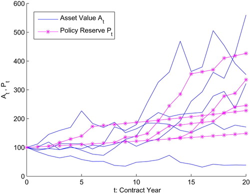$P_{t-1}$ and $B_{t-1}$), the analytical formula for $r_P\left(t\right)$ is⁵ (9) $r_P\left(t\right)=max\left\{r_G,\alpha \left(\frac{B_{t-1}}{P_{t-1}}-\gamma \right)\right\}.$(9) Figure 1 illustrates a simulation of five paths of the market value of invested assets $A_t$ and the hybrid policy reserve for a 20-year pension contract with a guaranteed interest rate $r_G=2\mathrm{\%}$. The above mechanism smooths the policy interest rate in the sense of having lower volatility.

Figure 1. Simulation of the Asset Value $A_t$ and Policy Reserve $P_t$ of the Pension Contract. Parameter set: $S_0=P_0=100$, $r=4\mathrm{\%}$, ${\sigma }_S=0.15$, $r_G=2\mathrm{\%}$.

The Equation (8(8) $P_t=P_{t-1}\times (1+r_P\left(t\right)),t=1,2,\dots ,T$(8) ) is updated as (10) $\begin{array}{rl}{P}_t& =P_{t-1}\left(1+max\left\{r_G,\alpha \left(\frac{B_{t-1}}{P_{t-1}}-\gamma \right)\right\}\right)\\ & =P_{t-1}\left(1+r_G+max\left\{0,\alpha \left(\frac{A_{t-1}-P_{t-1}}{P_{t-1}}-\gamma \right)-r_G\right\}\right)\end{array}$(10) In this mechanism, the bonus interest rate is an option element with strike value $r_G$, whereas $P_t$ is a path-dependent process with respect to $A_t$; as a result, we cannot find an analytical solution for the value. We can rewrite the Equation (10(10) $\begin{array}{rl}{P}_t& =P_{t-1}\left(1+max\left\{r_G,\alpha \left(\frac{B_{t-1}}{P_{t-1}}-\gamma \right)\right\}\right)\\ & =P_{t-1}\left(1+r_G+max\left\{0,\alpha \left(\frac{A_{t-1}-P_{t-1}}{P_{t-1}}-\gamma \right)-r_G\right\}\right)\end{array}$(10) ) as (11) $P_t=P_{t-1}\left(1+max\left\{r_G,\alpha \left(\frac{A_{t-1}}{P_{t-1}}-(1+\gamma )\right)\right\}\right)$(11) where the index $A_{t-1}/P_{t-1}$ is the well-known ‘funding ratio’ of the pension fund, and accordingly $1+\gamma$ is the ‘target funding ratio’.⁶ The above formulation is in fact a dynamic ‘profit-sharing’ mechanism that allocates potential extra profit based on the ratio of the assets and liabilities every year. Note that this profit-sharing mechanism is driven only by financial risks and not by actuarial risk.

2.2.2. Hybrid payoff and funding mechanism

To capture the fact that the liability side also depends on the actuarial risk, we add the mortality/longevity factor to the Grosen-Jorgensen setting.

We start by forming the hybrid payoff. Let $N_x\left(t\right)$ denote the cohort of the policyholders of age x + t at time t, with the initial cohort $N_x\left(0\right)$ of the policyholders who bought the policy at time t = 0. Each policyholder receives benefits of $P_T^{\left(h\right)}$ only if he/she is alive at maturity T (i.e. at age x + T), and zero otherwise. This arises from the implicit mechanism of insurance in the pension policy where a cohort pays the premium, but fewer people receive benefits.⁷ $P_T^{\left(h\right)}$ is the hybrid version of the policy reserve made by the hybrid crediting mechanism explained a paragraph later. The discounted general payoff at time T is then (12) $G(P_T,r_T,{\kappa }_T)=\left(e^{-{\int }_0^T{r}_t\mathrm{d}t}\right)\times P_T^{\left(h\right)}\times N_x\left(T\right).$(12) This general payoff is a function of the underlying risk drivers $A_T$, $P_T$, and $r_T$ for financial risks, and ${\kappa }_T$ for longevity risk modeled with the Lee–Carter model, as described in Subsection 2.1. However, note that at maturity T, the value of $P_T$ will be known by $A_{T-1}$ and $P_{T-1}$. Thus, we can omit $A_T$ in the payoff function and use $P_T$. Moreover, the payoff represents a European style contract without the surrender option before maturity.

Apart from the final payoff, we are also interested to know how mortality/longevity risk is involved in the funding and crediting mechanism. We look at this problem from the funding management point of view. In the Grosen-Jorgensen setting, the crediting mechanism follows a pure financial dynamics in each period. If the ratio of the assets to the policy reserves at the start of the period $(t-1,t)$ exceeds the target funding ratio of $1+\gamma$, the resulting interest is higher than the guaranteed interest rate of $r_G$. In that situation, the managers will consider paying the α portion of the excess assets to the remaining policyholders. Additionally, at maturity T, the total value of the policy reserve is $N_x\left(T\right)\times P_T$. Therefore, path-dependency is only due to the asset value and interest rate and not based on the number of survivors over the life of the contract. Pricing under the Grosen-Jorgensen mechanism implicitly postulates that the fund managers only take into account the time-zero expectation of the survivors at maturity T and do not change this perception based on the realization of $N_x\left(t\right)$ over the contract term.

The estimation or perception of the number of survivors at maturity, $N_x\left(T\right)$, depends on the realization of the time-t number of survivors, $N_x\left(t\right)$ over the contract period (which itself is based on the state of the longevity trend ${\kappa }_t$). We measure this time-t perception by the best-estimate of $N_x\left(T\right)$ at time t, denoted by $B{E}_t\left(N_x\right(T\left)\right)$, which is defined as its conditional expectation given the information available at time t, (13) $B{E}_t\left(N_x\left(T\right)\right)=\mathbb{E}\left[N_x\left(T\right)\mid N_x\left(t\right)\right].$(13) In fact, going forward over the valuation period to time t, the best-estimate value of $N_x\left(T\right)$ can be updated with the new information of the underlying process ${\kappa }_t$ and $N_x\left(t\right)$.

Suppose that the fund manager wants to calculate the policy interest rate at time t. Apart from the financial dynamics in the Grosen-Jorgensen setting, if at time t, $B{E}_t\left(N_x\right(T\left)\right)$ is higher than $B{E}_0\left(N_x\right(T\left)\right)$ (the initial perception of the fund manager on the terminal number of survivors), the situation will be riskier. In this situation, the fund manager will expect that the final collective policy reserve for the whole pension fund has to be divided among more survivors at time T, which means that the individual policy reserve at maturity, $P_T$ has to be less than the Grosen-Jorgensen policy reserve. This can be seen from the payoff formula in Equation (12(12) $G(P_T,r_T,{\kappa }_T)=\left(e^{-{\int }_0^T{r}_t\mathrm{d}t}\right)\times P_T^{\left(h\right)}\times N_x\left(T\right).$(12) ) where, if $N_x\left(T\right)$ increases, $P_T$ has to decrease so that the overall liability remains the same. This may convince the fund managers to promise a lower policy interest rate of $r_P$. To do so, they may pursue a more conservative policy for profit-sharing either by setting a higher target funding ratio ($1+\gamma$) or reducing the distribution ratio (α). This will automatically result in a lower bonus interest rate on top of $r_G$. On the other hand, if $B{E}_t\left(N_x\right(T\left)\right)<B{E}_0\left(N_x\right(T\left)\right)$, the updated estimation of the final survivors at maturity may convince the fund manager to set a more liberal profit-sharing policy by changing $1+\gamma$ or α. The reason is that he will expect fewer people at maturity to get the policy reserve $P_T$; this translates into higher policy reserve with a higher promised interest rate.

Using these facts, we can construct a hybrid crediting mechanism for the participating policy where the estimation of the final number of survivors affects crediting and profit sharing over the life of the contract. Under the hybrid mechanism, we assume that each survivor of the terminal cohort (at maturity T), $N_x\left(T\right)$, has an equal share of the fund's total assets and policy reserve. We define the hybrid funding ratio at time t as (14) $\mathrm{H}\mathrm{y}\mathrm{b}\mathrm{r}\mathrm{i}\mathrm{d}\mathrm{f}\mathrm{u}\mathrm{n}\mathrm{d}\mathrm{i}\mathrm{n}\mathrm{g}\mathrm{r}\mathrm{a}\mathrm{t}\mathrm{i}\mathrm{o}=\frac{B{E}_0\left(N_x\left(T\right)\right)A_t}{B{E}_t\left(N_x\left(T\right)\right)P_t}=\frac{\mathbb{E}\left[N_x\left(T\right)\mid N_x\left(0\right)\right]}{\mathbb{E}\left[N_x\left(T\right)\mid N_x\left(t\right)\right]}\times \frac{A_t}{P_t}.$(14) At each point of time t, the Grosen-Jorgensen funding ratio, $A_t/P_t$, is modified by the ratio of the time-zero best-estimate number of the final survivors to its time-t best-estimate.

By this hybrid funding ratio, we implicitly focus on the final survivors $N_x\left(T\right)$ against whom the fund bears liability. During the contract period at any time t, the final survivors own the ‘best-estimate’ value of $N_x\left(T\right)$ multiplied by the value of the asset $A_t$ or policy reserve $P_t$. The initial asset value and policy reserve for the whole cohort is then $B{E}_0\left(N_x\right(T\left)\right)\times A_0$ and $B{E}_0\left(N_x\right(T\left)\right)\times P_0$, respectively. However, as the investment asset evolves only through the dynamics of the financial market and not through the mortality/longevity trend, we only update the best-estimate of the final cohort for the policy reserve; we maintain our best estimate at time t = 0 for the asset side.

2.2.3. Technical component and profit sharing in hybrid mechanism

Let us denote all the quantities related to the hybrid mechanism with a superscript ‘${}^{\left(h\right)}$’. The modified formulation for hybrid policy interest rate is (15) $r_P^{\left(h\right)}\left(t\right)=max\left\{r_G,\alpha \left(\frac{B{E}_0\left(N_x\left(T\right)\right)}{B{E}_{t-1}\left(N_x\left(T\right)\right)}\times \frac{A_{t-1}}{P_{t-1}}-\left(1+\gamma \right)\right)\right\}.$(15) Note that technically $P_t^{\left(h\right)}$ is a function of $A_t$ and ${\kappa }_t$ as the underlying risk drivers. The hybrid funding ratio introduces a hybrid profit-sharing mechanism (year-on-year) dependent on two main components: the ‘investment component’ and the ‘technical component’. The investment component is a pure financial quantity that corresponds to the same funding ratio in the Grosen-Jorgensen setting, and the technical component is an actuarial ratio of the best-estimate number of survivors mentioned above as $B{E}_0\left(N_x\right(T\left)\right)/B{E}_{t-1}\left(N_x\right(T\left)\right)$. Hence, both investment and technical components are dynamic processes and make the payoff a path-dependent process for both investment assets and longevity trends through the above mechanism.

In Equation (15(15) $r_P^{\left(h\right)}\left(t\right)=max\left\{r_G,\alpha \left(\frac{B{E}_0\left(N_x\left(T\right)\right)}{B{E}_{t-1}\left(N_x\left(T\right)\right)}\times \frac{A_{t-1}}{P_{t-1}}-\left(1+\gamma \right)\right)\right\}.$(15) ), we can rewrite the target funding ratio $1+\gamma$ as a product of the technical component and a new ‘hybrid target buffer ratio’, $1+{\gamma }_{t-1}^{\left(h\right)}$, (16) $1+\gamma =\frac{B{E}_0\left(N_x\left(T\right)\right)}{B{E}_{t-1}\left(N_x\left(T\right)\right)}\times 1+{\gamma }_{t-1}^{\left(h\right)}$(16) This shows that even if γ in the managerial protocol may be determined as a constant value, technically at any time t it can be transformed into a dynamic process ${\gamma }_{t-1}^{\left(h\right)}$ under the hybrid crediting mechanism. Equation (15(15) $r_P^{\left(h\right)}\left(t\right)=max\left\{r_G,\alpha \left(\frac{B{E}_0\left(N_x\left(T\right)\right)}{B{E}_{t-1}\left(N_x\left(T\right)\right)}\times \frac{A_{t-1}}{P_{t-1}}-\left(1+\gamma \right)\right)\right\}.$(15) ) can be rewritten as follows (17) $r_P^{\left(h\right)}\left(t\right)=max\left\{r_G,\alpha \times \frac{B{E}_0\left(N_x\left(T\right)\right)}{B{E}_{t-1}\left(N_x\left(T\right)\right)}\left(\frac{A_{t-1}}{P_{t-1}}-\left(1+{\gamma }_{t+1}^{\left(h\right)}\right)\right)\right\}.$(17) where one can also consider $\alpha \times \left(B{E}_0\right(N_x\left(T\right)\left)/B{E}_{t-1}\right(N_x\left(T\right)\left)\right)$ as a new ‘dynamic distribution ratio’ under the hybrid profit-sharing mechanism.

Finally, the recursive formulas for the policy reserve in Equation (11(11) $P_t=P_{t-1}\left(1+max\left\{r_G,\alpha \left(\frac{A_{t-1}}{P_{t-1}}-(1+\gamma )\right)\right\}\right)$(11) ) is modified for the hybrid policy reserve as (18) $\begin{array}{rl}{P}_t^{\left(h\right)}& =P_{t-1}^{\left(h\right)}\times (1+r_P^{\left(h\right)}\left(t\right))\\ & =P_{t-1}^{\left(h\right)}\times \left(1+max\left\{r_G,\alpha \left(\frac{A_{t-1}}{P_{t-1}^{\left(h\right)}}-(1+{\gamma }_{t-1}^{\left(h\right)})\right)\right\}\right).\end{array}$(18) where at time t−1 by considering Equation (17(17) $r_P^{\left(h\right)}\left(t\right)=max\left\{r_G,\alpha \times \frac{B{E}_0\left(N_x\left(T\right)\right)}{B{E}_{t-1}\left(N_x\left(T\right)\right)}\left(\frac{A_{t-1}}{P_{t-1}}-\left(1+{\gamma }_{t+1}^{\left(h\right)}\right)\right)\right\}.$(17) ), the hybrid policy reserve, $P_{t-1}^{\left(h\right)}$ is obtained from the financial policy reserve as follows $P_{t-1}^{\left(h\right)}=\left(\frac{B{E}_{t-1}\left(N_x\left(T\right)\right)}{B{E}_0\left(N_x\left(T\right)\right)}\right)\times P_{t-1}.$

Example 2.1

Suppose the number of death $D_x\left(t\right)$ follows Poisson process with rate λ.⁸ Therefore, $\mathbb{E}\left[D_x\right(T\left)\right]=\lambda t$ and the cohort at time t is obtained as $N_x\left(t\right)=N_x\left(0\right)-D_x\left(t\right)$. The technical component (i.e. the ratio of the best-estimate terminal cohort) in Equation (14(14) $\mathrm{H}\mathrm{y}\mathrm{b}\mathrm{r}\mathrm{i}\mathrm{d}\mathrm{f}\mathrm{u}\mathrm{n}\mathrm{d}\mathrm{i}\mathrm{n}\mathrm{g}\mathrm{r}\mathrm{a}\mathrm{t}\mathrm{i}\mathrm{o}=\frac{B{E}_0\left(N_x\left(T\right)\right)A_t}{B{E}_t\left(N_x\left(T\right)\right)P_t}=\frac{\mathbb{E}\left[N_x\left(T\right)\mid N_x\left(0\right)\right]}{\mathbb{E}\left[N_x\left(T\right)\mid N_x\left(t\right)\right]}\times \frac{A_t}{P_t}.$(14) ) can be rewritten as, (19) $\begin{array}{rl}\frac{\mathbb{E}\left[N_x\left(T\right)\mid N_x\left(0\right)\right]}{\mathbb{E}\left[N_x\left(T\right)\mid N_x\left(t\right)\right]}& =\frac{\mathbb{E}\left[N_x\left(0\right)-D_x\left(T\right)\mid N_x\left(0\right)\right]}{\mathbb{E}\left[N_x\left(t\right)-D_x(T-t)\mid N_x\left(t\right)\right]}\\ & =\frac{N_x\left(0\right)-\mathbb{E}\left[D_x\left(T\right)\mid N_x\left(0\right)\right]}{N_x\left(t\right)-\mathbb{E}\left[D_x(T-t)\mid N_x\left(t\right)\right]}\\ & =\frac{N_x\left(0\right)-\lambda T}{N_x\left(t\right)-\lambda (T-t)}\\ & =\frac{N_x\left(0\right)-\lambda t-\lambda (T-t)}{N_x\left(t\right)-\lambda (T-t)}\\ & =\frac{\mathbb{E}\left[N_x\left(t\right)\right]-\lambda (T-t)}{N_x\left(t\right)-\lambda (T-t)}.\end{array}$(19) Note that in the third equation conditioning on $N_x\left(t\right)$ is equivalent to condition on $D_x\left(t\right)$, hence, the conditional expected value can be written in terms of $\lambda t$.⁹ The last equation represents a clear interpretation of the technical component; The numerator $\mathbb{E}\left[N_x\right(t\left)\right]-\lambda (T-t)$ includes ‘the expected number of survivors’ at time t, while the denominator $N_x\left(t\right)-\lambda (T-t)$ has ‘the realized number of survivors’ at time t, both deducted by the expected number of survivors at maturity T.

For the Poisson cohort, using Equation (19(19) $\begin{array}{rl}\frac{\mathbb{E}\left[N_x\left(T\right)\mid N_x\left(0\right)\right]}{\mathbb{E}\left[N_x\left(T\right)\mid N_x\left(t\right)\right]}& =\frac{\mathbb{E}\left[N_x\left(0\right)-D_x\left(T\right)\mid N_x\left(0\right)\right]}{\mathbb{E}\left[N_x\left(t\right)-D_x(T-t)\mid N_x\left(t\right)\right]}\\ & =\frac{N_x\left(0\right)-\mathbb{E}\left[D_x\left(T\right)\mid N_x\left(0\right)\right]}{N_x\left(t\right)-\mathbb{E}\left[D_x(T-t)\mid N_x\left(t\right)\right]}\\ & =\frac{N_x\left(0\right)-\lambda T}{N_x\left(t\right)-\lambda (T-t)}\\ & =\frac{N_x\left(0\right)-\lambda t-\lambda (T-t)}{N_x\left(t\right)-\lambda (T-t)}\\ & =\frac{\mathbb{E}\left[N_x\left(t\right)\right]-\lambda (T-t)}{N_x\left(t\right)-\lambda (T-t)}.\end{array}$(19) ), $r_P^{\left(h\right)}\left(t\right)$ can be rearranged as (20) $r_P^{\left(h\right)}\left(t\right)=max\left\{r_G,\alpha \left(\frac{\mathbb{E}\left[N_x\left(t\right)\right]-\lambda (T-t)}{N_x\left(t\right)-\lambda (T-t)}\right)\left(\frac{A_{t-1}}{P_{t-1}}-\left(1+\gamma \right)\right)\right\}$(20) where we implicitly assumed that $1+{\gamma }^{\left(h\right)}=\left(\frac{\mathbb{E}\left[N_x\right(t\left)\right]-\lambda (T-t)}{N_x\left(t\right)-\lambda (T-t)}\right)(1+\gamma ).$

The hybrid crediting mechanism adds some extra insights into the Grosen-Jorgensen setting. Suppose in year t, the realized number of survivors is larger than the expected number of survivors; i.e. $N_x\left(t\right)>\mathbb{E}\left[N_x\right(t\left)\right]$. This deviation can be seen as a ‘local realization of the longevity risk’. Then, the technical component will act on the investment component of the funding ratio as a decreasing factor and, on average, decreases the policy interest rate closer to $r_G$. That means that when there is a sign of the longevity risk in the portfolio, the hybrid mechanism in Equation (20(20) $r_P^{\left(h\right)}\left(t\right)=max\left\{r_G,\alpha \left(\frac{\mathbb{E}\left[N_x\left(t\right)\right]-\lambda (T-t)}{N_x\left(t\right)-\lambda (T-t)}\right)\left(\frac{A_{t-1}}{P_{t-1}}-\left(1+\gamma \right)\right)\right\}$(20) ) will impose a ‘conservative crediting’ on the policy interest rate. On the opposite side, if the realized number of survivors is less than the expected number of survivors, i.e. $N_x\left(t\right)<\mathbb{E}\left[N_x\right(t\left)\right]$, the technical component is larger than one and will act as an enlarging factor of the investment component, resulting in a higher policy interest rate. Comparing to the Grosen-Jorgensen mechanism, using the technical component and the hybrid crediting mechanism creates more liberal reactions of the fund to interest crediting. It also provides a more realistic indexation by adding the extra effect from the actuarial risk dynamics on profit sharing.¹⁰

To calculate the technical component, $\mathbb{E}\left[N_x\right(T)\mid N_x(0\left)\right]/\mathbb{E}\left[N_x\right(T)\mid N_x(t\left)\right]$ under the Lee–Carter model, we need to obtain the expected value of the stochastic survival probability, ${}_T{p}_x\left(\overrightarrow{\kappa }\right)$, given the vector $\overrightarrow{\kappa }=({\kappa }_0,\dots ,{\kappa }_T)$. Recalling the Lee–Carter dynamic for the force-or-mortality in Equation (1(1) $\ln {\mu }_x\left(t\right)={\alpha }_x+{\text{β}}_x{\kappa }_t$(1) ), the formulation for ${}_T{p}_x\left(\overrightarrow{\kappa }\right)$ will be (22) $\begin{array}{rl}{}_T{p}_x\left(\overrightarrow{\kappa }\right)& =\prod _{j=0}^{T-1}{p}_{x+j}\left({\kappa }_j\right)\\ & =\exp \left(-\sum _{j=0}^{T-1}{\mu }_{x+j}\left({\kappa }_j\right)\right)\\ & =\exp \left(-\sum _{j=0}^{T-1}\exp \left({\alpha }_{x+j}+{\text{β}}_{x+j}{\kappa }_j\right)\right)\end{array}$(22) Based on the ${\kappa }_t$ dynamics in Lee-Carter model and using Itô formula, one can find the stochastic process for ${}_T{p}_x$. However, its distribution is still unknown. Knowing the stochastic dynamics of ${}_T{p}_x$, it is also possible to calculate its conditional expected value given the information available at t<T (See Shreve 2010 for justification on this). However, to stay in the scope, we ignore doing so and use simulation techniques instead in the numerical phase.

3. Pricing framework

The payoff in Equation (12(12) $G(P_T,r_T,{\kappa }_T)=\left(e^{-{\int }_0^T{r}_t\mathrm{d}t}\right)\times P_T^{\left(h\right)}\times N_x\left(T\right).$(12) ) is an example of the wide variety of derivatives that are a combined function of the underlying financial and actuarial risks. We consider the mortality/longevity (with underlying risk process ${\kappa }_t$) as an unhedgeable (or partially hedgeable) actuarial risk, where the no-arbitrage argument cannot be applied due to market incompleteness. Instead, we use one of the actuarial premium principles to price it. Generally, the premium principles are non-linear and static operators without any market-consistency and time-consistency properties. On the other hand, the interest rate ($r_t$) and investment asset ($A_t$) (and accordingly the policy reserve $P_t$) are assumed to be fully hedgeable financial risks that are tradable in an arbitrage-free and complete market. Hence, with the fundamental theorem of asset pricing, the price of the derivative made of $A_t$ and $r_t$ is a conditional expectation under the unique risk-neutral martingale measure $\mathbb{Q}$.

We want to price the participating policy simultaneously under the market-consistency and time-consistency properties. By definition, the pricing operator Π is market-consistent; if for any financial payoff $H^S$ and the mixed (financial and actuarial) one G, we have (23) $\mathrm{\Pi }\left[G+H^S\right]=\mathrm{\Pi }\left[G\right]+{\mathbb{E}}^{\mathbb{Q}}\left[H^S\right].$(23) The market-consistent price operator possesses a more general notion of the translation invariance for the financial payoff $H^S$ and is the best possible hedging strategy for the whole position. As a result of applying Π for the sum of replicable and non-replicable payoffs, as the liquid and perfectly replicable part of the position carries the market risk, it should be priced under the no-arbitrage operator. Additionally, the total price is the summation of this price and the price of Π of G. The more technical definition of the market-consistency can be found in Malamud et al. (2008), Pelsser & Stadje (2014), and Salahnejhad & Pelsser (2020).

Moreover, by definition Π is time-consistent over the valuation period $[t,T]$, if for two risks X and Y, $\mathrm{\Pi }[T,X]>\mathrm{\Pi }[T,Y]$, then for all $t\le s<T$, $\mathrm{\Pi }[s,X]>\mathrm{\Pi }[s,Y]$. Jobert & Rogers (2008) showed that time-consistency can be obtained by a backward iteration of the one-period price over the possible sub-intervals over the valuation period. Hence, $\mathrm{\Pi }[t,X]$ is time-consistent price of the position $f\left(X_T\right)$ at time t, if for all t<s<T (24) $\mathrm{\Pi }\left[t,T,f\left(X_T\right)\right]=\mathrm{\Pi }[t,s,\mathrm{\Pi }\left[s,T,f\left(X_T\right)\right]].$(24) Note that, as an especial case, ${\mathbb{E}}^{\mathbb{Q}}$ is a time-consistent and market-consistent operator.

3.1. Two-step actuarial valuation

Pelsser & Stadje (2014) show that any market-consistent operator can be constructed by a ‘two-step valuation’ that splits the actuarial and no-arbitrage financial pricing operators for every valuation period. For a pricing operator that is time-consistent over only a finite number of points in the valuation period, the two-step valuation preserves the market-consistency on the same points. Using this property, Salahnejhad & Pelsser (2020) mixed the two-step actuarial valuation and backward iteration to introduce an applied representation for time-consistent and market-consistent price in discrete-time and continuous-time.

Let $(\mathrm{\Omega },\mathcal{F},\mathbb{P})$ be the underlying probability space with the filtration $({\mathcal{F}}_t{)}_{t\ge 0}$ over $[0,T]$. Suppose $({\mathcal{F}}_t^A{)}_{t\ge 0}$, $({\mathcal{F}}_t^r{)}_{t\ge 0}$ and $({\mathcal{G}}_t^A{)}_{t\ge 0}$ denote the filtrations generated by the policy reserve $P_t$, interest rate $r_t$, and mortality trend ${\kappa }_t$, which all are subsets of $\mathcal{F}$. We form the set ${\mathcal{F}}_t^S=\sigma ({\mathcal{F}}_t^A\cup {\mathcal{F}}_t^r)$ as the filtration for the combination of financial risk drivers $P_t$ and $r_t$ and ${\mathcal{G}}_t=\sigma ({\mathcal{F}}_t^S\cup {\mathcal{G}}_t^A)$, as the hybrid filtration generated by the general payoff which provides the information flow of the financial and actuarial risks together at time t.

3.1.1. Two-step operator

Suppose we are at time t and let ${\pi }_t$ be the price of the payoff in Equation (12(12) $G(P_T,r_T,{\kappa }_T)=\left(e^{-{\int }_0^T{r}_t\mathrm{d}t}\right)\times P_T^{\left(h\right)}\times N_x\left(T\right).$(12) ) conditional on the information available at time t. Salahnejhad & Pelsser (2020) consider the operator for only two risk drivers (one financial and the other actuarial). We extend the same framework for three risk drivers (two financial and one actuarial) where, the market-consistent price of the participating policy at time t<T is obtained by the following two-step operator (25) ${\pi }_t(A_T,r_T,{\kappa }_T)={\mathbb{E}}^{\mathbb{Q}}\left[{\mathrm{\Pi }}^{\mathbb{P}}\left[\left(e^{-{\int }_t^T{r}_{s}ds}\right)\times P_T^{\left(h\right)}\times N_x\left(T\right)\mid \sigma ({\mathcal{G}}_t^A\cup {\mathcal{F}}_T^S)\right]\mid \sigma ({\mathcal{G}}_t^A\cup {\mathcal{F}}_t^S)\right]$(25) where Π can act as one of the actuarial premium principles. It is easy to examine that the above two-step operator satisfies Equation (23(23) $\mathrm{\Pi }\left[G+H^S\right]=\mathrm{\Pi }\left[G\right]+{\mathbb{E}}^{\mathbb{Q}}\left[H^S\right].$(23) ).

The above two-step operator is a one-period valuation consisting of an ‘Inner Step’ and an ‘Outer Step’. In the inner step, we assume that we know the full financial information related to the policy reserve and term structure of the interest rate up to and including maturity T, but our information regarding the mortality trend κ is limited to time t<T. Hence, the only randomness comes from ${\kappa }_T$. Here, we use a slightly different version of hybrid σ-algebra $\mathcal{G}$ where there is a time lag between the financial filtration up to T and actuarial filtration up to t<T. We can show the hybrid filtration as ${\mathcal{G}}_{T,t}=\sigma ({\mathcal{F}}_T^S\cup {\mathcal{G}}_t^A)$. In the following, by fixing $A_T$ and $r_T$, we use ${\mathrm{\Pi }}^{\mathbb{P}}$ as the actuarial premium principle under the real-world measure $\mathbb{P}$ and calculate the actuarial part of the payoff conditional on ${\mathcal{G}}_t^A$ (or equivalently conditioned on ${\mathcal{G}}_{T,t}$). In the two-step valuation, this is the inner step and its result will be a function of the policy reserve $P_T$ and the short rate $r_t$ from t up to T, shown by $G^S(P_T,r_T)$. As we assumed, $G^S(P_T,r_T)$ is a fully hedgeable and tradable position in the no-arbitrage and complete market. Hence, in the outer step, we use the no-arbitrage pricing operator and take the expectation conditional on the available operators on their financial information ${\mathcal{F}}_t^S$ under the unique risk-neutral measure $\mathbb{Q}$.

We assume that $A_t$, $r_t$, and ${\kappa }_t$ have Markov property and are adapted to the corresponding information flows ${\mathcal{F}}_t^A$, ${\mathcal{F}}_t^r$, and ${\mathcal{G}}_t^A$. Thus, for simplicity, we will use the value of the processes instead of the related filtrations in the pricing operators. Nevertheless, the alternative notation (with the use of filtrations) is also valid for all the two-step conditional operators.

Now, we also want to include the time-consistency to the two-step valuation in Equation (25(25) ${\pi }_t(A_T,r_T,{\kappa }_T)={\mathbb{E}}^{\mathbb{Q}}\left[{\mathrm{\Pi }}^{\mathbb{P}}\left[\left(e^{-{\int }_t^T{r}_{s}ds}\right)\times P_T^{\left(h\right)}\times N_x\left(T\right)\mid \sigma ({\mathcal{G}}_t^A\cup {\mathcal{F}}_T^S)\right]\mid \sigma ({\mathcal{G}}_t^A\cup {\mathcal{F}}_t^S)\right]$(25) ). Let us choose the Standard-Deviation premium principle as the actuarial price operator Π in the inner step. We assume that the price is time-consistent on finite predictable points of time $t\in \{0,1,2,\dots ,T-1,T\}$. Therefore, in a multi-period setting, we apply the backward iteration of the two-step actuarial valuation on an annual basis¹¹ starting from $[T-1,T]$ and ending up at $[0,1]$. So, the time-consistent and market-consistent Standard-Deviation pricing operator for the participating policy payoff in Equation (12(12) $G(P_T,r_T,{\kappa }_T)=\left(e^{-{\int }_0^T{r}_t\mathrm{d}t}\right)\times P_T^{\left(h\right)}\times N_x\left(T\right).$(12) ) is $\begin{array}{rl}{\pi }_t(A_{t+1},r_{t+1},{\kappa }_{t+1})& ={\mathbb{E}}^{\mathbb{Q}}[{\mathbb{E}}^{\mathbb{P}}\left[\left(e^{-{\int }_t^{t+1}{r}_s\mathrm{d}s}\right){\pi }_{t+1}(A_{t+1},r_{t+1},{\kappa }_{t+1})\mid {\kappa }_t,A_{t+1},r_{t+1}\right]\\ & +\text{β}\sqrt{\mathbb{V}{\mathrm{a}\mathrm{r}}^{\mathbb{P}}\left[\left(e^{-{\int }_t^{t+1}{r}_s\mathrm{d}s}\right){\pi }_{t+1}(A_{t+1},r_{t+1},{\kappa }_{t+1})\mid {\kappa }_t,A_{t+1},r_{t+1}\right]}\mid {\kappa }_t,A_t,r_t]\end{array}$ with terminal condition (26) ${\pi }_T(A_T,r_T,{\kappa }_T)=\left(e^{-{\int }_{T-1}^T{r}_s\mathrm{d}s}\right)\times P_T^{\left(h\right)}\times N_x\left(T\right)$(26) where $\text{β}>0$ is the loading coefficient. The operator is constructed by using the similar time-consistency definition in Equation (24(24) $\mathrm{\Pi }\left[t,T,f\left(X_T\right)\right]=\mathrm{\Pi }[t,s,\mathrm{\Pi }\left[s,T,f\left(X_T\right)\right]].$(24) ), where the payoff applicable in each time-step of the form $(t,t+1)$ (in the two-step operator) is the one-period two-step value obtained one time-step further in $(t+1,t+2)$. The integral $\left({\int }_t^{t+1}{r}_s\mathrm{d}s\right)$ represents the t-forward interest rate accumulated over the time-step $(t,t+1)$.

By recalling Equation (25(25) ${\pi }_t(A_T,r_T,{\kappa }_T)={\mathbb{E}}^{\mathbb{Q}}\left[{\mathrm{\Pi }}^{\mathbb{P}}\left[\left(e^{-{\int }_t^T{r}_{s}ds}\right)\times P_T^{\left(h\right)}\times N_x\left(T\right)\mid \sigma ({\mathcal{G}}_t^A\cup {\mathcal{F}}_T^S)\right]\mid \sigma ({\mathcal{G}}_t^A\cup {\mathcal{F}}_t^S)\right]$(25) ), the one-period Standard-Deviation actuarial price will be defined as, (27) $\begin{array}{rl}{\pi }_t(A_T,r_T,{\kappa }_T)& ={\mathbb{E}}^{\mathbb{Q}}[{\mathbb{E}}^{\mathbb{P}}\left[\left(e^{-{\int }_{T-1}^T{r}_s\mathrm{d}s}\right)\times P_T^{\left(h\right)}\times N_x\left(T\right)\mid {\kappa }_t,A_T,r_T\right]\\ & +\text{β}\sqrt{T-t}\sqrt{\mathbb{V}{\mathrm{a}\mathrm{r}}^{\mathbb{P}}\left[\left(e^{-{\int }_t^T{r}_s\mathrm{d}s}\right)\times P_T^{\left(h\right)}\times N_x\left(T\right)\mid {\kappa }_t,A_T,r_T\right]}\mid {\kappa }_t,A_t,r_t]\end{array}$(27) where the coefficient $\sqrt{T-t}$ is multiplied to β to match the dimensionality problem of the square root function. For more details, see the related discussion in (Salahnejhad & Pelsser 2016).

3.1.2. (In)dependence structure

Due to the use of conditional operators, the two-step valuation is by construction consistent with the dependence structure between financial and actuarial risk drivers. If there is a non-zero correlation between financial and actuarial risk drivers, the actuarial risk is hedged partially via financial risk. That means that in Equation (25(25) ${\pi }_t(A_T,r_T,{\kappa }_T)={\mathbb{E}}^{\mathbb{Q}}\left[{\mathrm{\Pi }}^{\mathbb{P}}\left[\left(e^{-{\int }_t^T{r}_{s}ds}\right)\times P_T^{\left(h\right)}\times N_x\left(T\right)\mid \sigma ({\mathcal{G}}_t^A\cup {\mathcal{F}}_T^S)\right]\mid \sigma ({\mathcal{G}}_t^A\cup {\mathcal{F}}_t^S)\right]$(25) ) knowing the full financial information ${\mathcal{F}}_T^S$, we also know part of the actuarial information ${\mathcal{G}}_T^A$. Therefore, if in the inner step we fix the Markov process $P_T$ and $r_T$, we have some information to forecast the value of ${\kappa }_T$. As we assume $P_T$ and $r_T$ are fully hedgeable in the market in the outer step, a part of the position with underlying ${\kappa }_T$ can be hedged by the arbitrage-free operator ${\mathbb{E}}^{\mathbb{Q}}$ due to the common information available in the financial market. This is discussed by Salahnejhad & Pelsser (2020) for the continuous-time limit of the time-consistent two-step Variance and Standard-Deviation operators. They show that a function of the correlation between financial and actuarial risks adjusts the stochastic process for the underlying actuarial risk. The adjustment plays the role of a hedge cost to hedge the actuarial risk process partially in the market. In their study, the continuous-time limit of the market-consistent and the time-consistent price is represented by a partial differential equation that must be solved numerically, as it doesn't have an explicit analytical solution.

However, in reality it is difficult to find a justification that the level and shape of the term structure and/or value of the investment asset can affect the level or trend of the mortality or vice versa. Salahnejhad & Pelsser (2020) consider a unit-linked product with a structure similar to that in the Grosen-Jorgensen case in Equation (11(11) $P_t=P_{t-1}\left(1+max\left\{r_G,\alpha \left(\frac{A_{t-1}}{P_{t-1}}-(1+\gamma )\right)\right\}\right)$(11) ), where $P_T$ is the final payoff $P_T\times N_x\left(T\right)$, which is built based on a pure financial procedure. Due to the factorized structure of the payoff, for an independent policy reserve and mortality risks the inner and outer operators in the two-step operator can be split into the product of the operators as below (28) ${\pi }_t(P_T,{\kappa }_T)=e^{-r(T-t)}{\mathbb{E}}^{\mathbb{Q}}\left[P_T\mid {\mathcal{F}}_t^S\right]\times {\mathrm{\Pi }}^{\mathbb{P}}\left[N_x\left(T\right)\mid {\mathcal{G}}_t^A\right]$(28) where there is no shared information generated by the two risk drivers.¹² They showed that in a continuous-time mortality model, applying the time-consistency for the actuarial operator ${\mathrm{\Pi }}^{\mathbb{P}}$ and the fact that the expectation operator $\mathbb{E}$ is time-consistent, the two-step Standard-Deviation operator in Equation (28(28) ${\pi }_t(P_T,{\kappa }_T)=e^{-r(T-t)}{\mathbb{E}}^{\mathbb{Q}}\left[P_T\mid {\mathcal{F}}_t^S\right]\times {\mathrm{\Pi }}^{\mathbb{P}}\left[N_x\left(T\right)\mid {\mathcal{G}}_t^A\right]$(28) ) will be rearranged as (29) ${\pi }_t(P_T,{\kappa }_T)=e^{-r(T-t)}{\mathbb{E}}^{\mathbb{Q}}\left[P_T\mid P_t\right]\times {\mathbb{E}}^{\mathbb{S}}\left[N_x\left(T\right)\mid {\kappa }_t^{\mathbb{S}}\right]$(29) where ${\mathbb{E}}^{\mathbb{S}}[\cdot \mid {\kappa }_t^{\mathbb{C}}]$ is the conditional expectation with respect to information available at time t under the underlying risk-adjusted process (30) $\mathrm{d}{\kappa }_t^{\mathbb{S}}=\left({\mu }_{\kappa }-\text{β}{\sigma }_{\kappa }\right)\mathrm{d}t+{\sigma }_{\kappa }\mathrm{d}{W}_t^{\mathbb{S},\kappa }.$(30) The result is based on the continuous-time limit of the Standard-Deviation principle when $\mathrm{\Delta }t\to 0$ by Salahnejhad & Pelsser (2016).

We set the independence assumption between the actuarial risk ${\kappa }_t$ and the financial risks $A_t$ and $r_t$, while $A_t$ and $r_t$ are correlated. Despite the independence assumption, the payoff in Equation (12(12) $G(P_T,r_T,{\kappa }_T)=\left(e^{-{\int }_0^T{r}_t\mathrm{d}t}\right)\times P_T^{\left(h\right)}\times N_x\left(T\right).$(12) ) cannot be factorized as a product of the financial and actuarial risks, as $P_T^{\left(h\right)}$ is a hybrid path-dependent function of $A_t$ and ${\kappa }_t$. Hence, giving an explicit solution for the time-consistent two-step Standard-Deviation value is not possible, and we have to calculate the price numerically.

4. Numerical method

In this section, we explain the numerical techniques that we implement to calculate the time-consistent and market-consistent actuarial price of the participating contract. The numerical method is a combination of Monte-Carlo simulation and the regression-based methods to calculate the values in the two-step actuarial operator and necessary conditional expectations. We focus on generating the scenarios of the payoff in Equation (12(12) $G(P_T,r_T,{\kappa }_T)=\left(e^{-{\int }_0^T{r}_t\mathrm{d}t}\right)\times P_T^{\left(h\right)}\times N_x\left(T\right).$(12) ) by simulating the underlying risk drivers: investment asset value $A_t$, interest rate $r_t$, and the longevity trend ${\kappa }_t$ for $t\in \{0,1,\dots ,T\}$. To do so, we calculate the hybrid policy interest rate $r_P^{\left(h\right)}\left(t\right)$, and the policy reserve $P_t^{\left(h\right)}$ via Equations (15(15) $r_P^{\left(h\right)}\left(t\right)=max\left\{r_G,\alpha \left(\frac{B{E}_0\left(N_x\left(T\right)\right)}{B{E}_{t-1}\left(N_x\left(T\right)\right)}\times \frac{A_{t-1}}{P_{t-1}}-\left(1+\gamma \right)\right)\right\}.$(15) ) and (18(18) $\begin{array}{rl}{P}_t^{\left(h\right)}& =P_{t-1}^{\left(h\right)}\times (1+r_P^{\left(h\right)}\left(t\right))\\ & =P_{t-1}^{\left(h\right)}\times \left(1+max\left\{r_G,\alpha \left(\frac{A_{t-1}}{P_{t-1}^{\left(h\right)}}-(1+{\gamma }_{t-1}^{\left(h\right)})\right)\right\}\right).\end{array}$(18) ), respectively. To achieve time-consistency, we use the backward iteration method to repeat the one-period two-step actuarial value over the valuation period with regression-based methods.

4.1. Simulation of $r_P^{\left(h\right)}$ and $P_t^{\left(h\right)}$

Using the correlation matrix in Equation (7(7) $\overrightarrow{\rho }=\left(\begin{array}{ccc}1& {\rho }_{\kappa ,r}& {\rho }_{\kappa ,A}\\ {\rho }_{\kappa ,r}& 1& {\rho }_{A,r}\\ {\rho }_{\kappa ,A}& {\rho }_{A,r}& 1\end{array}\right)$(7) ) and its Cholesky decomposition, we simulate a three-dimensional Brownian motion $(W_t^{\kappa },W_t^A,W_t^r{)}^{\mathrm{\top }}$ for $t\in 0,1,\dots ,T$.¹³ Then, we use the dynamics in Subsection 2.1 to construct a sequence of investment asset $A_t$, interest rate $r_t$, and longevity trend ${\kappa }_t$. For the interest rate $r_t$, we first generate the following Ornstein–Uhlenbeck process (31) $\mathrm{d}{X}_t=-a{X}_t\mathrm{d}t+\sigma \mathrm{d}{W}_t^r$(31) where $X_0=0$ and $r_t=X_t+\alpha \left(t\right)$. $\alpha \left(t\right)$ can be determined by fitting $X_t$ to an initial term structure from the market and finally get the tractability parameter $\theta \left(t\right)$ in Equation (6(6) $\mathrm{d}{r}_t=\left[\theta \left(t\right)-a{r}_t\right]\mathrm{d}t+{\sigma }_r\mathrm{d}{W}_t^r$(6) ). See Pelsser (2000) for more details on transformation of $r_t$ and $X_t$ and obtaining the tractability parameter $\theta \left(t\right)$. For each risk driver, we simulate n replication, each useful for one path. Therefore, the final output will be three matrices for $A_t$, $r_t$ and ${\kappa }_t$, with dimension $n\times (T+1)$.

To simulate the payoff in Equation (12(12) $G(P_T,r_T,{\kappa }_T)=\left(e^{-{\int }_0^T{r}_t\mathrm{d}t}\right)\times P_T^{\left(h\right)}\times N_x\left(T\right).$(12) ) we should generate $N_x\left(t\right)$ and $r_P^{\left(h\right)}\left(t\right)$. As $N_x\left(t\right)=N_x\left(0\right){\times }_t{p}_x$ and the initial cohort $N_x\left(0\right)$ is known, $N_x\left(t\right)$ can be easily generated using the simulation path of ${\kappa }_t$ process and calculating the survival probability by Equation (22(22) $\begin{array}{rl}{}_T{p}_x\left(\overrightarrow{\kappa }\right)& =\prod _{j=0}^{T-1}{p}_{x+j}\left({\kappa }_j\right)\\ & =\exp \left(-\sum _{j=0}^{T-1}{\mu }_{x+j}\left({\kappa }_j\right)\right)\\ & =\exp \left(-\sum _{j=0}^{T-1}\exp \left({\alpha }_{x+j}+{\text{β}}_{x+j}{\kappa }_j\right)\right)\end{array}$(22) ). This results in an $n\times (T+1)$ matrix containing n paths of $N_x\left(t\right)$.

The core item to simulate $r_P^{\left(h\right)}\left(t\right)$ is the technical component $B{E}_0\left(N_x\right(T\left)\right)/B{E}_t\left(N_x\right(T\left)\right)$ and the best-estimate value via the conditional expectation of $N_x\left(T\right)$ given the underlying processes/information at time t. Assuming ${\kappa }_t$ and $N_x\left(t\right)$ as Markov processes, they contain the full information up to and including time t. We use the shorter notation ${\mathbb{E}}_t\left[N_x\right(T\left)\right]$ instead of $\mathbb{E}\left[N_x\right(T)\mid N_x(t\left)\right]$. We assume that we have the estimated values of the age-specific parameters $a_x$ and $b_x$ in the Lee–Carter model for all possible ages.

The numerical implementation should be consistent with the implementation of the backward iteration of the one-period valuation. In the simulation stage above, each of the n realization of $N_x\left(T\right)$ is built by one sequence of the underlying process ${\kappa }_t$ (or $N_x\left(t\right)$) that forms a random path for $N_x\left(t\right)$ over time. To establish the price calculation in the backward iteration method for each typical time-step $(t-1,t)$ for n realization of the state variable (e.g. $N_x\left(t\right)$), the numerical procedure must deliver n realization of the calculated value (e.g. $E_{t-1}\left[N_x\right(t\left)\right]$) that can be later used as the input for the time-step $(t-2,t-1)$.¹⁴ Later, we will discuss this method in Section 4.2. Note that n realization of $E_{t-1}\left[N_x\right(t\left)\right]$ is also required to deliver n replications of $r_P^{\left(h\right)}\left(t\right)$ and $P_t^{\left(h\right)}$.

We start from time t = 0, where the expectation of the number of final survivors can be easily obtained by substituting the best-estimate of ${\kappa }_t$, i.e. $\mathbb{E}[{\kappa }_t\mid {\kappa }_0]={\kappa }_0+{\mu }_{\kappa }t$ into Equation (22(22) $\begin{array}{rl}{}_T{p}_x\left(\overrightarrow{\kappa }\right)& =\prod _{j=0}^{T-1}{p}_{x+j}\left({\kappa }_j\right)\\ & =\exp \left(-\sum _{j=0}^{T-1}{\mu }_{x+j}\left({\kappa }_j\right)\right)\\ & =\exp \left(-\sum _{j=0}^{T-1}\exp \left({\alpha }_{x+j}+{\text{β}}_{x+j}{\kappa }_j\right)\right)\end{array}$(22) ). The simpler method is taking an average of $N_x\left(T\right)$ that implicitly is generated with information available at time t = 0. We move to t = 1, where in the numerical implementation we have n realization of $N_x\left(T\right)$, and given n values of ${\kappa }_1$ (or $N_x\left(1\right)$), we have to deliver n values of ${\mathbb{E}}_1\left[N_x\right(T\left)\right]$. This means that for each given value of the underlying Markov process ${\kappa }_1$ or $N_x\left(1\right)$, we only have one realization of $N_x\left(T\right)$ while we need at least two observations to be able to calculate the average as the estimation of the conditional expectation.¹⁵ The regression-based methods in the next subsection provide an efficient solution to this problem.

4.2. Regression-based methods

Let $h(T,{\kappa }_T)$ be the payoff function contingent on ${\kappa }_T$. The target function is defined as $f(t,{\kappa }_t)=\mathbb{E}\left[h\right(T,{\kappa }_T)\mid {\kappa }_t]$ for $0\le t\le T$. We assume that the payoff h is a square-integrable random variable given by $L^2(\mathrm{\Omega },{\mathcal{G}}_t^A,\mathbb{P})$. The conditional expectation (i.e. $f(t,{\kappa }_t$) can be obtained by an infinite series of basis functions of ${\kappa }_t$ (32) $\mathbb{E}\left[h\right(T,{\kappa }_T)\mid {\kappa }_t]=f(t,{\kappa }_t)=\sum _{k=0}^{\mathrm{\infty }}{a}_k{e}_k\left({\kappa }_t\right)$(32) with $e_k$ as the basis functions of the underlying risk driver at time t<T and coefficients $a_k\in \mathbb{R}$.

The function f can be estimated by a finite number of terms K in the above summation as (33) $f(t,{\kappa }_t)\approx f_K(t,{\kappa }_t)=\sum _{k=0}^K{a}_k{e}_k\left({\kappa }_t\right)$(33) where the least-square estimator of $f(t,{\kappa }_t)$, denoted by $\hat{f}$, can be calculated under the following argument, (34) $\hat{f}(t,{\kappa }_t)={\mathrm{a}\mathrm{r}\mathrm{g}\mathrm{m}\mathrm{i}\mathrm{n}}_{{\overrightarrow{a}}_k}\sum _{i=1}^n{\left[f_i(t,{\kappa }_t)-\sum _{k=0}^K{a}_k{e}_k\left({\kappa }_t\right(i\left)\right)\right]}^2$(34) where $f_i$ and ${\kappa }_t\left(i\right)$ denote the ith realization of f and ${\kappa }_t$.

The Equations (33(33) $f(t,{\kappa }_t)\approx f_K(t,{\kappa }_t)=\sum _{k=0}^K{a}_k{e}_k\left({\kappa }_t\right)$(33) ) and (34(34) $\hat{f}(t,{\kappa }_t)={\mathrm{a}\mathrm{r}\mathrm{g}\mathrm{m}\mathrm{i}\mathrm{n}}_{{\overrightarrow{a}}_k}\sum _{i=1}^n{\left[f_i(t,{\kappa }_t)-\sum _{k=0}^K{a}_k{e}_k\left({\kappa }_t\right(i\left)\right)\right]}^2$(34) ) formulate a regression model to estimate the target function known as the ‘Least-Square Monte-Carlo (LSMC)’ and/or ‘regression-now’. The regression methods and the corresponding basis functions were proposed by Madan & Milne (1994) and later by Carriere (1996). Longstaff & Schwartz (2001) use this method to price American options, and later Stentoft (2004) show the convergence of the LSMC estimator to the correct price, and discuss the convergence rate based on the properties of the conditional expectation. Glasserman & Yu (2004b) introduce another version of the regression-based methods called ‘regression-later estimator’. In the regress-later method, one should first fit the payoff function with the underlying risk driver, both at time T and then (using the additivity property of the expectation, take the expectation operator into the summation and) substitute for the analytical solution of the conditional expectation (if available). Unlike the regression-now method, regression later is model-independent since changing the pricing measure the regression coefficient, and the fitting function does not change.

Both regression-based estimators are consistent with the path-dependence of the hybrid policy reserve $P_t^{\left(h\right)}$ and possess the key features to operate in line with the backward iteration procedure. Using the regression coefficients over each time-step, they can deliver a prediction of the target function (response variable) with n replications from a vector of payoff (independent variable) with n replications.

Now, we calculate ${\mathbb{E}}_t\left[N_x\right(T\left)\right]$ with the regression-based method in Subsection 4.1. For a general case of 0<t<T, suppose that $N_x\left(T\right)$ can be estimated via polynomial basis functions of the underlying risk driver ${\kappa }_T$, (35) ${\hat{N}}_x\left(T\right)=\sum _{k=0}^K\widehat{a_k}{\kappa }_T^k$(35) Taking the conditional expectation, given ${\kappa }_t$, we have the estimation of the expectation of the conditional survivors as (36) $\begin{array}{rl}\hat{\mathbb{E}}\left[N_x\left(T\right)\mid {\kappa }_t\right]& =\mathbb{E}\left[\sum _{k=0}^K\widehat{a_k}{\kappa }_T^k\mid {\kappa }_t\right]\end{array}$(36) (37) $\begin{array}{rl}& =\sum _{k=0}^K\widehat{a_k}\mathbb{E}\left[{\kappa }_T^k\mid {\kappa }_t\right]\end{array}$(37) However, as ${\kappa }_T$ is normally distributed, the analytical solution of $\mathbb{E}[{\kappa }_T^k\mid {\kappa }_t]$ is easy to find. This is a useful application of the regression-later method to estimate ${\mathbb{E}}_t\left[N_x\right(T\left)\right]$. The method can be repeatedly used in the backward iteration. In such setting, the fitting function and the regression coefficients remain the same for all iterations. As such, to make sure the payoff ($N_x\left(T\right)$) is well fitted, the $R^2$ in the regression should be sufficiently high.

Another alternative to estimate ${\mathbb{E}}_t\left[N_x\right(T\left)\right]$ is using the regression-now method with either of the following models, (38) $\hat{\mathbb{E}}\left[N_x\left(T\right)\mid {\kappa }_t\right]=\sum _{k=0}^K\widehat{a_k}{\kappa }_t^k$(38) where ${\kappa }_t$ is used directly as the underlying risk driver to directly estimate ${\mathbb{E}}_t\left[N_x\right(T\left)\right]$, or (39) $\hat{\mathbb{E}}\left[N_x\left(T\right)\mid {\kappa }_t\right]=\sum _{k=0}^K\widehat{b_k}{N}_x^k\left(t\right).$(39) where $\widehat{b_k}$ is the estimation of the new regression coefficients for the regressors $N_x^k\left(t\right)$.

Note that, based on Equation (22(22) $\begin{array}{rl}{}_T{p}_x\left(\overrightarrow{\kappa }\right)& =\prod _{j=0}^{T-1}{p}_{x+j}\left({\kappa }_j\right)\\ & =\exp \left(-\sum _{j=0}^{T-1}{\mu }_{x+j}\left({\kappa }_j\right)\right)\\ & =\exp \left(-\sum _{j=0}^{T-1}\exp \left({\alpha }_{x+j}+{\text{β}}_{x+j}{\kappa }_j\right)\right)\end{array}$(22) ), $N_x\left(t\right)$ is by construction a function of all ${\kappa }_j$ values for 0<j<t over $(0,T)$, while ${\kappa }_t$ only reflects part of the available information to estimate $N_x\left(T\right)$. The same reasoning applies to the regression-later formula in Equation (35(35) ${\hat{N}}_x\left(T\right)=\sum _{k=0}^K\widehat{a_k}{\kappa }_T^k$(35) ), where ${\kappa }_T$ as the independent variable in the polynomial only possesses the last piece of information used for $N_x\left(T\right)$. In this sense, we think the regression-now method in Equation (39(39) $\hat{\mathbb{E}}\left[N_x\left(T\right)\mid {\kappa }_t\right]=\sum _{k=0}^K\widehat{b_k}{N}_x^k\left(t\right).$(39) ) is superior to the other options mentioned here. However, in a partitioned time period $t\in 1,2,\dots ,T$, to estimate the first conditional expectation ${\mathbb{E}}_{t=1}\left[N_x\right(T\left)\right]$, the regress-now estimator in Equation (39(39) $\hat{\mathbb{E}}\left[N_x\left(T\right)\mid {\kappa }_t\right]=\sum _{k=0}^K\widehat{b_k}{N}_x^k\left(t\right).$(39) ) is not applicable as we have a single value for $N_x\left(0\right)$. For t = 1, we will exceptionally use the regression-later estimator that does not have the above-mentioned shortage, and ${\kappa }_1$ provides the full information needed to calculate $N_x\left(1\right)$. Therefore, in this paper, we use a combination of the regression-now and regression-later methods to calculate the T vector of the technical component of the hybrid profit-sharing mechanism over the contract term.

Now, we have all the necessary materials in Equation (15(15) $r_P^{\left(h\right)}\left(t\right)=max\left\{r_G,\alpha \left(\frac{B{E}_0\left(N_x\left(T\right)\right)}{B{E}_{t-1}\left(N_x\left(T\right)\right)}\times \frac{A_{t-1}}{P_{t-1}}-\left(1+\gamma \right)\right)\right\}.$(15) ) to simulate $r_P^{\left(h\right)}\left(t\right)$ and $P_t^{\left(h\right)}$. At time t = 1, we use $A_0$ and $P_0$ to calculate $r_P^{\left(h\right)}\left(1\right)=max[r_G,\alpha (A_0/P_0-(1+\gamma )\left)\right]$¹⁶ and the vector $P_1^{\left(h\right)}=P_0\times r_P^{\left(h\right)}\left(1\right)$. At time t = 2, we use the simulated vector of $A_1$, the vector $P_1^{\left(h\right)}$ we obtained in the previous period and the vector of ${\mathbb{E}}_0\left[N_x\right(T\left)\right]/{\mathbb{E}}_1\left[N_x\right(T\left)\right]$ that we estimated early by the regression-based methods. Using Equation (15(15) $r_P^{\left(h\right)}\left(t\right)=max\left\{r_G,\alpha \left(\frac{B{E}_0\left(N_x\left(T\right)\right)}{B{E}_{t-1}\left(N_x\left(T\right)\right)}\times \frac{A_{t-1}}{P_{t-1}}-\left(1+\gamma \right)\right)\right\}.$(15) ), we calculate $r_P^{\left(h\right)}\left(2\right)$ and $P_2^{\left(h\right)}$ and continue to do so until time T. By the simulated sequential vectors up to $r_T$, $N_x\left(T\right)$, and $P_t^{\left(T\right)}$, we can calculate the payoff in Equation (12(12) $G(P_T,r_T,{\kappa }_T)=\left(e^{-{\int }_0^T{r}_t\mathrm{d}t}\right)\times P_T^{\left(h\right)}\times N_x\left(T\right).$(12) ) and start to calculate the pricing operators.

4.3. Price calculation by LSMC

The Standard-Deviation actuarial price consists of the first two moments of the discounted payoff; therefore, we can use the LSMC to implement the estimation of the price operator. We use the same method that we introduced in Salahnejhad & Pelsser (2020) with two underlying risk drivers (one financial and one actuarial). However, in this paper, we have one more financial risk driver, and hence, we extend the method to be used for three risk drivers. $r_t$ and $A_t$ are the underlying financial risk drivers while $N_x\left(t\right)$ is the actuarial risk driver.¹⁷ We start from the maturity T as the beginning point of the backward iteration and apply the two-step Standard-deviation operator in Equation (26(26) ${\pi }_T(A_T,r_T,{\kappa }_T)=\left(e^{-{\int }_{T-1}^T{r}_s\mathrm{d}s}\right)\times P_T^{\left(h\right)}\times N_x\left(T\right)$(26) ) over the interval $(T-1,T)$. The discounted payoff is (40) $f_T^{\left(h\right)}=\exp \left(-{\int }_{T-1}^T{r}_s\mathrm{d}s\right)P_T^{\left(h\right)}\times N_x\left(T\right)$(40) where the discounting factor is the price of the zero-coupon bond issued on T−1 with maturity T.

Suppose, the valuation period $(0,T)$ is partitioned as $\{0,1,2,\dots ,T\}$ and we have the simulated paths over the partitioned times for $A_t$, $r_t$, $N_x\left(t\right)$, and $P_t^{\left(h\right)}$ with n replications. The pricing procedure is as follows,

• Start from maturity T and value over $(T-1,T)$. In the inner step, the conditional expectation of the payoff and the squared payoff, can be estimated through the following regressions, (41a) $\begin{array}{rl}& \widehat{{\mathbb{E}}^{\mathbb{P}}}\left[\exp \left(-{\int }_{T-1}^T{r}_s\mathrm{d}s\right)P_T^{\left(h\right)}\times N_x\left(T\right)|A_T,r_T,{\kappa }_{T-1}\right]=\sum _{k=0}^{K-1}{\widehat{a_k}}^{(1,T)}{e}_k(A_T,r_T,{\kappa }_{T-1})\end{array}$(41a) (41b) $\begin{array}{rl}& \widehat{{\mathbb{E}}^{\mathbb{P}}}\left[{\left(\exp \left(-{\int }_{T-1}^T{r}_s\mathrm{d}s\right)P_T^{\left(h\right)}\times N_x\left(T\right)\right)}^2|A_T,r_T,{\kappa }_{T-1}\right]=\sum _{k=0}^{K-1}{\widehat{a_k}}^{(2,T)}{e}_k(A_T,r_T,{\kappa }_{T-1})\end{array}$(41b) where the regression coefficients ${\widehat{a_k}}^{(1,T)}$ and ${\widehat{a_k}}^{(2,T)}$ are estimated under the argument of minimizing the squared error.

• Calculate the Conditional premium ${\pi }^{\mathrm{s}}(A_T,r_T,{\kappa }_{T-1})$ in the inner step, (42) ${\pi }^{\mathrm{s}}\left(A_T,r_T,{\kappa }_{T-1}\right)=\widehat{{\mathbb{E}}^{\mathbb{P}}}\left[f_T^{\left(h\right)}\right]+\text{β}\sqrt{\widehat{{\mathbb{E}}^{\mathbb{P}}}\left[(f_T^{\left(h\right)}{)}^2\right]-{\left(\widehat{{\mathbb{E}}^{\mathbb{P}}}\left[f_T^{\left(h\right)}\right]\right)}^2}.$(42) This value is the result of the inner step and is used as the payoff for the outer step.

• We apply the outer step and estimate the arbitrage-free price (i.e. the conditional expectation) with the following regression equation, (43) $\begin{array}{rl}{\pi }^{\mathrm{s}}\left(A_{T-1},r_{T-1},{\kappa }_{T-1}\right)& =\widehat{{\mathbb{E}}^{\mathbb{Q}}}\left[{\pi }^{\mathrm{s}}\left(A_T,r_T,{\kappa }_{T-1}\right))\mid A_{T-1},r_{t-1}{\kappa }_{T-1}\right]\\ & =\sum _{k=0}^{K-1}{\widehat{b_k}}^{\left(T\right)}{e}_{{\pi }^{\mathrm{s}}}(A_{T-1},r_{T-1},{\kappa }_{T-1})\end{array}$(43) where again $b_k^{\left(T\right)}$ is estimated by minimizing the squared error. Note that going backward in time, ${\pi }^{\mathrm{s}}(A_{T-1},r_{T-1},{\kappa }_{T-1})$ now will be used as a new payoff vector at time T−1 to implement the two-step valuation over $(T-2,T-1)$ and calculate the value at T−2.

• Repeat the above three steps, for all typical time steps of the form $(t,t+1)$, going backward in time over the partitioned valuation period up to time zero.

5. Numerical results

In this section, we provide the results of the numerical methods described in the previous section to calculate the time-consistent two-step actuarial price of the participating policy.

We obtain the price as a single premium for a participating policy with a single payoff. The initial cohort is assumed to be $N_x\left(0\right)=\mathrm{100,000}$ equal males and females with the age of x = 40 years at the start of the contract, and different maturities are set up to T = 30 years(with main focus on 5, 10, 20, and 30 years). We calibrate the Lee–Carter model by using the Dutch aggregated mortality tables for men and women during 1960–2006 (47 years) and obtain the parameters of the mortality trend process $k_t$ as follows: The initial value ${\kappa }_0=-24.5637$, the drift ${\mu }_{\kappa }=-0.8089$, and the diffusion coefficient ${\sigma }_{\kappa }=1.4734$. The age-specified parameters $a_x$ and $b_x$ can be found in Appendix.

To calibrate the Hull–White interest rate model, we use 30-year annual zero rates in the Euro area released by the European Central Bank (ECB) until January 2, 2006.¹⁸ The rates are calculated based on the prices of the AAA-rated euro area central government bonds. We set the mean reversion parameter of the Hull–White model as a = 0.04 and work with a variety of the volatility parameter ${\sigma }_r$ between $(0.01,0.1)$.

We work with the Monte-Carlo simulation of n = 1000 scenario paths for the underlying risk drivers. For every time-step in the backward iteration, the number of paths to implement the regression-based methods remains constant. We then repeat the simulation N = 100 times, which gives us the standard error and the confidence interval around the estimated price.

5.1. Time-consistent and market-consistent price

We simulate the hybrid payoff in Equation (12(12) $G(P_T,r_T,{\kappa }_T)=\left(e^{-{\int }_0^T{r}_t\mathrm{d}t}\right)\times P_T^{\left(h\right)}\times N_x\left(T\right).$(12) ) using the method described in Subsection 4.1, and calculate the time-consistent two-step Standard-Deviation actuarial price in Equation (26(26) ${\pi }_T(A_T,r_T,{\kappa }_T)=\left(e^{-{\int }_{T-1}^T{r}_s\mathrm{d}s}\right)\times P_T^{\left(h\right)}\times N_x\left(T\right)$(26) ) based on the simulation of the policy interest rate in Equation (15(15) $r_P^{\left(h\right)}\left(t\right)=max\left\{r_G,\alpha \left(\frac{B{E}_0\left(N_x\left(T\right)\right)}{B{E}_{t-1}\left(N_x\left(T\right)\right)}\times \frac{A_{t-1}}{P_{t-1}}-\left(1+\gamma \right)\right)\right\}.$(15) ). In Equation (7(7) $\overrightarrow{\rho }=\left(\begin{array}{ccc}1& {\rho }_{\kappa ,r}& {\rho }_{\kappa ,A}\\ {\rho }_{\kappa ,r}& 1& {\rho }_{A,r}\\ {\rho }_{\kappa ,A}& {\rho }_{A,r}& 1\end{array}\right)$(7) ), we set the correlation of the financial risk drivers ${\rho }_{A,r}=0.25$ and assume the correlation of ${\kappa }_t$ with $A_t$ and $r_t$ equal to zero. Later, we will study the effect of the correlation on the time-consistent and market-consistent price.

As we required both time-consistency and market-consistency for the desired price, it is important to compare our Standard-Deviation actuarial price with the other alternative time-consistent market-consistent price, which is the two-step, expectation operator.¹⁹ As we mentioned before, the expectation operator is intrinsically time-consistent due to the tower property. Thus, we do not need to apply the backward iteration over the valuation period. We only use the one-period valuation method. Hence, both values are time-consistent and market-consistent.

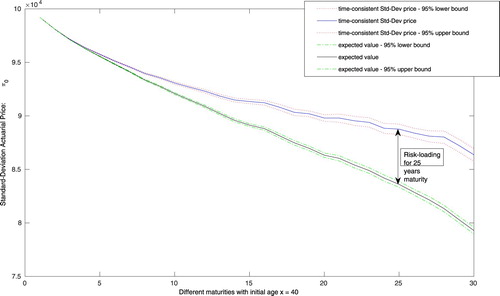
Figure 2, exhibits the result of the time-consistent and market-consistent Standard Deviation actuarial price and the one-period expectation price operator for different maturities of $T=\{1,2,\dots ,30\}$. The difference between the two values is the time-consistent and market-consistent actuarial risk-loading added to the expectation to penalize for the possible future unexpected losses. The risk-loading for the short-term contracts ($0.2\mathrm{\%}$ for a 5-years contract) is small. But it increases when the maturity is longer ($6.2\mathrm{\%}$ for a 25-years and $8.9\mathrm{\%}$ for a 30-years contract). We observe a reasonable $95\mathrm{\%}$ confidence interval for the price, where for the longest maturity (30-years), the lower/upper bound has a $0.7\mathrm{\%}$ difference with the point estimation.

Figure 2. Time-consistent and market-consistent Standard-Deviation actuarial price vs. discounted expected value of the hybrid payoff of the participating contract with 95% confidence interval and different maturities $T=1,2,\dots ,30$. Parameter set: $A_0=P_0=100$, ${\sigma }_A=15\mathrm{\%}$, ${\sigma }_r=1\mathrm{\%}$, ${\rho }_{A,r}=0.25$, $r_G=2\mathrm{\%}$, $\alpha =0.3$, $\gamma =0.25$, n = 1000, N = 100.

In Salahnejhad & Pelsser (2020), we have discussed the ‘time-consistency risk premium’ as the difference between the one-period and time-consistent (multi-period) two-step actuarial prices. The one-period actuarial price is formulated by adding a portion of the standard deviation to the expected value of the discounted payoff (also one-period) in Equation (27(27) $\begin{array}{rl}{\pi }_t(A_T,r_T,{\kappa }_T)& ={\mathbb{E}}^{\mathbb{Q}}[{\mathbb{E}}^{\mathbb{P}}\left[\left(e^{-{\int }_{T-1}^T{r}_s\mathrm{d}s}\right)\times P_T^{\left(h\right)}\times N_x\left(T\right)\mid {\kappa }_t,A_T,r_T\right]\\ & +\text{β}\sqrt{T-t}\sqrt{\mathbb{V}{\mathrm{a}\mathrm{r}}^{\mathbb{P}}\left[\left(e^{-{\int }_t^T{r}_s\mathrm{d}s}\right)\times P_T^{\left(h\right)}\times N_x\left(T\right)\mid {\kappa }_t,A_T,r_T\right]}\mid {\kappa }_t,A_t,r_t]\end{array}$(27) ), while the time-consistent price comes from Equation (26(26) ${\pi }_T(A_T,r_T,{\kappa }_T)=\left(e^{-{\int }_{T-1}^T{r}_s\mathrm{d}s}\right)\times P_T^{\left(h\right)}\times N_x\left(T\right)$(26) ). The surplus of the one-period Standard-Deviation price over the expected value is the ‘one-period risk-loading’, and the surplus of the time-consistent standard-deviation price over the one-period Standard-deviation price is the ‘time-consistency risk premium’. The sum of the two surpluses is the risk-loading referred to in the previous paragraph. $\text{Risk-loading}=\text{One-period risk-loading}+\text{Time-consistency risk premium}$ Since we emphasize the requirement of time-consistency with a market-consistent price, it is interesting to know how the risk-loading will be partitioned between the time-consistency risk premium and the one-period risk-loading.

Table 1 shows that more than 90% of the risk-loading is the time-consistency risk premium and only a small portion is the one-period Standard-Deviation loading. Note that for each maturity, the result is obtained out of an annual backward iteration of the two-step valuation along the valuation period until time zero. None of the longer maturity prices are obtained using the values of the shorter maturities.

Table 1. The values of the participating contract with different maturities for the initial cohort of $N_{40}\left(0\right)=1000$, and the ratio of the one-period risk-loading and time-consistency risk premium on top of the expected value of the contract.

	T
Two-step price	5	10	15	20	25	30
Expected-value	95,558.6	92,088.3	89,138.6	86,328.2	83,600.2	79,284.6
One-period std-dev	95,574.6	92,123.6	89,198.5	86,422.7	83,746.6	79,513.5
Time-consistent std-dev	95,752.7	93,072.1	91,342.2	89,802.1	88,761.6	86,365.5
One-period risk-loading	0.02%	0.04%	0.07%	0.11%	0.19%	0.31%
Time-consistency premium	0.19%	1.03%	2.40%	3.91%	5.99%	8.62%
Total risk-loading	0.20%	1.07%	2.47%	4.02%	6.17%	8.93%
Ratio of TC premium	91.8%	96.4%	97.2%	97.2%	97.0%	96.5%

Notes: Parameter set: $A_0=P_0=100$, ${\sigma }_A=15\mathrm{\%}$, ${\sigma }_r=1\mathrm{\%}$, ${\rho }_{A,r}=0.25$, $r_G=2\mathrm{\%}$, $\alpha =0.3$, $\gamma =0.25$, n = 1000, N = 100.

In general, different factors can affect the price of the participating contract with a hybrid payoff and crediting (profit-sharing) mechanisms. Among all factors, when the maturity increases, the asset value increases, and the discount factor and the number of survivors decreases, on average. We also have the one-period risk-loading and the time-consistency risk premium that increases in maturity and can enlarge the price over time. Among the above factors, in Figure 2, we observe that the discount factor and the number of survivors dominate the others and decrease the price when the maturity increases. Moreover, regardless of the maturity, recalling Equation (15(15) $r_P^{\left(h\right)}\left(t\right)=max\left\{r_G,\alpha \left(\frac{B{E}_0\left(N_x\left(T\right)\right)}{B{E}_{t-1}\left(N_x\left(T\right)\right)}\times \frac{A_{t-1}}{P_{t-1}}-\left(1+\gamma \right)\right)\right\}.$(15) ), the other effectual factors are the distribution ratio (α), the volatility of the investment asset (${\sigma }_A$), and the volatility of the interest rate (${\sigma }_r$) that positively affects price, and the target buffer ratio (γ) that negatively affects the price. See Grosen & Jorgensen (2000) for an explanation of these factors and their effects on the value of the contract. Higher α means a more liberal profit-sharing policy of the fund managers, while a higher γ means that the fund managers follow a more conservative policy for profit sharing and the policyholders can get part of the excess investment return on top of the guaranteed rate $r_G$ only if the funding ratio is very high.

Table 2 studies the effect of the distribution ratio (α), the target buffer ratio (γ), and the volatility of the investment asset (${\sigma }_A$) on the price of the contract. For each ${\sigma }_A$, α, γ, and maturity from the set $T\in \{5,10,15,20,25,30\}$, we provided the price of the contract and summarized the average standard error of the price for different amounts of γ obtained from the Monte-Carlo simulation. The table has two vertical panels, each of which provides the results for two levels of the investment asset volatility. The prices and standard errors are provided for ${\sigma }_A=15\mathrm{\%}$ and ${\sigma }_A=30\mathrm{\%}$. There are also horizontal panels where each represents the prices and average Standard error for a level of the distribution ratio (α). Within each horizontal panel, the prices and standard errors vary for different levels of the target buffer ratio (γ) and maturities (T).

Table 2. Time-consistent and market-consistent actuarial Standard-Deviation price of the participating contract for different levels of the investment asset volatility ${\sigma }_A=15\mathrm{\%}$ and ${\sigma }_A=30\mathrm{\%}$, different profit-sharing mechanism parameters, α and γ, and different maturities.

	${\sigma }_A$
	$15\mathrm{\%}$						$30\mathrm{\%}$
	γ					Average	γ					Average
T	0	0.1	0.2	0.3	0.4	SE	0	0.1	0.2	0.3	0.4	SE
$\alpha =0.00$												$\times {10}^3$
5	94.26	94.27	94.26	94.25	94.26	0.006	94.26	94.27	94.27	94.26	94.26	0.006
10	85.83	85.84	85.85	85.87	85.86	0.013	85.85	85.86	85.86	85.87	85.86	0.013
15	76.94	76.88	76.89	76.94	76.91	0.021	76.91	76.93	76.92	76.91	76.89	0.021
20	68.46	68.42	68.46	68.45	68.43	0.027	68.43	68.45	68.42	68.45	68.41	0.027
25	60.37	60.35	60.34	60.37	60.40	0.031	60.31	60.37	60.32	60.36	60.30	0.030
30	52.41	52.56	52.42	52.44	52.45	0.032	52.43	52.35	52.39	52.40	52.35	0.032
$\alpha =0.25$
5	100.05	97.98	96.59	95.74	95.21	0.022	107.60	105.02	103.10	101.71	100.52	0.068
10	101.87	98.12	95.40	93.29	91.68	0.063	120.43	115.68	112.15	109.54	106.56	0.225
15	103.29	98.52	94.91	91.81	89.47	0.114	133.28	127.66	123.48	117.31	114.58	0.509
20	104.86	99.18	94.66	91.26	87.99	0.178	146.35	141.26	134.83	132.03	123.14	1.079
25	106.55	100.58	95.40	90.92	87.37	0.254	162.18	157.46	149.20	139.81	133.20	1.485
30	108.25	101.22	95.53	90.86	86.58	0.331	178.48	171.80	161.91	154.61	152.12	2.669
$\alpha =0.50$
5	105.62	101.70	99.05	97.41	96.28	0.036	118.06	114.04	110.61	107.69	105.42	0.115
10	110.96	105.10	100.81	97.65	94.98	0.086	137.55	131.57	125.60	120.98	117.21	0.294
15	114.26	107.49	102.12	98.04	94.77	0.150	156.39	148.97	141.29	133.64	129.02	0.675
20	117.90	110.18	103.60	98.48	95.11	0.203	179.73	167.95	159.50	149.98	146.04	1.488
25	121.00	112.51	105.36	100.05	95.26	0.303	200.93	186.44	177.99	169.76	159.04	2.667
30	122.76	114.97	106.86	101.05	95.89	0.431	221.87	204.17	191.02	189.64	179.77	4.590
$\alpha =0.75$
5	109.57	104.51	100.90	98.67	97.19	0.045	126.31	120.38	115.85	112.19	109.08	0.146
10	116.30	109.46	104.01	100.30	97.26	0.101	148.92	141.18	134.75	128.39	123.68	0.376
15	120.71	112.65	106.56	101.60	97.81	0.167	170.79	160.18	153.34	144.43	138.92	0.723
20	124.39	115.80	108.98	102.82	98.38	0.253	192.94	180.63	171.58	163.86	153.30	1.423
25	127.58	118.55	111.08	104.00	99.42	0.294	221.98	204.01	193.13	175.89	172.74	2.616
30	131.10	120.77	113.22	105.77	100.89	0.439	249.12	224.07	218.43	199.43	188.98	4.602
$\alpha =1.00$
5	112.62	106.47	102.36	99.71	97.89	0.057	132.43	125.54	119.94	115.73	112.18	0.150
10	120.25	112.51	106.62	102.20	99.00	0.103	158.97	148.17	140.54	134.00	129.29	0.396
15	124.74	115.95	109.41	103.94	99.83	0.167	182.01	168.92	161.26	152.57	145.70	0.807
20	129.33	120.01	112.19	105.94	101.06	0.259	205.23	190.34	179.50	171.97	163.48	1.563
25	133.28	122.71	115.29	108.41	102.45	0.334	234.10	220.18	204.77	193.60	182.59	2.870
30	136.39	125.25	117.24	110.28	104.54	0.501	254.05	243.41	225.48	208.44	209.52	4.156

Notes: Parameter set: $A_0=P_0=100$, ${\sigma }_A=15\mathrm{\%}$, ${\sigma }_r=1\mathrm{\%}$, ${\rho }_{A,r}=0.25$, $r_G=2\mathrm{\%}$, n = 1000, N = 100.

We first consider the first panel where $\alpha =0$ and no bonus/surplus over the guaranteed rate of $r_G$ is distributed each year. That turns the participating contract into a ‘longevity bond’ sold to a cohort of $N_x\left(0\right)$ and deactivates the hybrid crediting mechanism too. Since there is no profit-sharing and the overall term structure is higher than $r_G$, the price in this panel will always remain below the par value, $P_0=100$. The crediting rate is then $r_G$. Therefore, changing the volatility of the investment asset, from ${\sigma }_A=15\mathrm{\%}$ to ${\sigma }_A=30\mathrm{\%}$, plays no role in price and its standard error. Compare the values on the right and left half side of the panel.

When α rises, there will be a positive profit-sharing in the contract that is also called ‘bonus option’. As a result, the value difference between the lower panels and the first panel (where $\alpha =0$) provides the price of the bonus option. Going down over the panels with a higher α, the bonus (profit-sharing) policy gets more liberal and increases the price of the bonus option.

When $\gamma =0$, it means that the fund managers do not hold any buffer reserve for the fund, and as long as the assets are over the policy reserves, the policyholders will have a chance to receive returns. Considering the right columns of each panel over higher amounts of γ, the bonus (profit-sharing) policy of the fund managers gets more conservative. Therefore the price of the contract decreases and a lower price is reported for the bonus option.

In the lower panels, when the higher distribution ratio allows for more freedom to achieve higher crediting interest rate, the price of the bonus option (and therefore the price of the contract) increases for all maturities as expected. On the other hand, when the investment asset becomes more volatile and volatility increases from $15\mathrm{\%}$ to $30\mathrm{\%}$ in the right half, the prices also increase. The price growth due to change in the volatility is more for the longer maturities. Compare for example the numbers in the panel with $\alpha =0.50$ and $\gamma =0.2$. For the maturity T = 5, the price goes from $99.05\times {10}^3$ for ${\sigma }_A=15\mathrm{\%}$ to $110.61\times {10}^3$ equivalent to $11.7\mathrm{\%}$ growth. However, if we consider the maturity T = 30, the price increases from $106.86\times {10}^3$ to $191.02\times {10}^3$, exhibiting a $78.8\mathrm{\%}$ growth. In this table, the volatility of the Hull–White interest rate model (${\sigma }_r$) is fixed to ${\sigma }_r=0.05$. In Subsection 5.2, we study the effect of the interest rate factor and its volatility on the price.

To have a better view of the effect of the funding policy over different maturities, we provide the above results for the time-consistent and market-consistent price over time. We compare the value of the contract with three combined levels of the distribution ratio, α, and the funding ratio, $1+\gamma$ that represent three different funding policy scenarios, including:

• Precautionary policy, where we set $\alpha =25\mathrm{\%}$ and $1+\gamma =130\mathrm{\%}$,

• Moderate policy, where we set $\alpha =50\mathrm{\%}$ and $1+\gamma =115\mathrm{\%}$, and

• Liberal policy, where we set $\alpha =75\mathrm{\%}$ and $1+\gamma =105\mathrm{\%}$.

In the precautionary policy, for example, the fund management requires a relatively high funding ratio, $1+\gamma =130\mathrm{\%}$, and will distribute a relatively low portion, $\alpha =25\mathrm{\%}$ of the extra buffer on top of the guaranteed rate $r_G=2\mathrm{\%}$ as the bonus if that holds. The opposite happens with the liberal policy. The rest of the parameters stay unchanged for Table 2.

The comparative values for the abovementioned funding policies and their evolution over different maturities are provided in Figure 3. The precautionary funding policy requires a lower risk premium and price as compared to liberal and moderate policies. The positive effect of the maturity T is reflected where higher maturities provide higher compensation against the effect of the discount factor. Likewise, prices with higher asset return volatility ${\sigma }_A$, dominate those with lower ones. The only exception is the case where the price under the liberal policy with ${\sigma }_A=15\mathrm{\%}$ is higher than the price under the precautionary policy with ${\sigma }_A=30\mathrm{\%}$ for maturities lower under T = 14. Let us compare the results over time, for example, when ${\sigma }_A=15\mathrm{\%}$. The price under the liberal policy for a contract with maturity T = 15 is approximately $26.6\mathrm{\%}$ higher than a precautionary policy. For a contract with T = 30 years, this difference is around $40.3\mathrm{\%}$.

Figure 3. Comparing the effect of the funding policy on the time-consistent and market-consistent Standard-Deviation of the participating contract, simulated under Precautionary, Moderate, and Liberal policies and two different level of the asset return volatility ${\sigma }_A=15\mathrm{\%}$ and ${\sigma }_A=30\mathrm{\%}$ over different maturities $T=\{1,2,\dots ,30\}$. Other parameters: $A_0=P_0=100$, ${\sigma }_A=15\mathrm{\%}$, ${\sigma }_r=1\mathrm{\%}$, ${\rho }_{A,r}=0.25$, $r_G=2\mathrm{\%}$, $\alpha =0.3$, $\gamma =0.25$, n = 1000, N = 100.

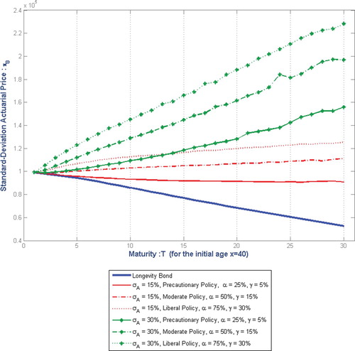
The reference value for the prices under any funding policy is the price of the longevity bond when there is no profit-sharing, shown with the thick blue line in Figure 3. This price, as the guaranteed part of the liability, is the same for all funding policies (shown with the green and red lines) and decreases with longer maturities due to the effect of the discount factor. The surplus over this value is the time-consistent and market-consistent price of the option element of the contract that increases for longer maturities. Comparing the price for maturity T = 25, and comparing to the price of the longevity bond equal to ${60.35}^3$, the price of the option element (surplus return on top of $r_G$) for ${\sigma }_A=15\mathrm{\%}$, adds $51\mathrm{\%}$ to the longevity bond price for precautionary policy and respectively $80\mathrm{\%}$ and $103\mathrm{\%}$ for moderate and liberal policy. Therefore, under the liberal policy, the time-consistent and market-consistent price of the participating contract is more than double the price of the longevity bond. The price of the option element for the higher asset volatility ${\sigma }_A=30\mathrm{\%}$ adds $136\mathrm{\%}$, $200\mathrm{\%}$, and $249\mathrm{\%}$ to the longevity bond price under the precautionary policy, moderate policy, and liberal policy respectively. Thus, as we double the asset return volatility (${\sigma }_A$ from $15\mathrm{\%}$ to $30\mathrm{\%}$), the price of the option element increases more than double for all policies. This shows that the option element is highly sensitive to the volatility (${\sigma }_A$). The result holds for other maturities as well and hence holds over time.

5.2. The effect of the stochastic interest rate

We assess the effect of the stochastic interest rate on the value of the contract by comparing the values obtained by the stochastic term-structure under the Hull–White interest rate model in Equation (6(6) $\mathrm{d}{r}_t=\left[\theta \left(t\right)-a{r}_t\right]\mathrm{d}t+{\sigma }_r\mathrm{d}{W}_t^r$(6) ) and the deterministic term-structure where in the same model ${\sigma }_r=0$. For the stochastic interest rate, we provide the values for three levels of the interest rate volatility ${\sigma }_r=\{0.01,0.05,0.1\}$ that, together with the deterministic rate, gives four different version of the price to compare. We compare the effect for the discounted expected value²⁰ and the time-consistent and market-consistent Standard-Deviation price. The rest of the parameters are fixed as mentioned in the beginning of this section.

Table 3 represents the percentage difference between the values obtained by the stochastic and deterministic interest rates. The left part of the table delivers the percentage difference for the discounted expected value, while the right part represents the percentage difference for the Standard-deviation price. The differences are reported for three levels of ${\sigma }_r$ and three maturities T = 20, 25, 30. In general, as all the observed percentage differences are positive, we conclude that the effect of the stochastic interest rate can be captured by a special risk-loading on top of the value obtained by deterministic interest rate; let us call it ‘interest rate loading’. At first glance, comparing to the expected values (left part of the table), the time-consistent and market-consistent Standard-Deviation price (right part of the table) shows a slightly higher interest rate loading on the price. We observe that the interest rate volatility ${\sigma }_r$ is the factor that causes a dramatic increase in the interest rate loading. For example for T = 25, increasing ${\sigma }_r$ from 0.01 to 0.1 (10 times larger) causes the interest rate loading for the Standard-Deviation price to increase from $0.29\mathrm{\%}$ to $11.05\mathrm{\%}$ (around 38 times larger). However, generally for the lower level of ${\sigma }_r=0.01$, the interest rate loading for all maturities stays very small: between (0.15–0.35)% for the expected value and (0.19–.46)% for Standard-Deviation price. This is useful for practitioners as they can expect to be close to the reasonable price with a stochastic interest rate (even if calculated with a deterministic term structure) if the market for the interest rate derivatives is not volatile and in their model ${\sigma }_r$ is estimated as a small quantity. This significantly reduces the numerical algorithm required in the calculation phase. The interest rate loading also increases by the maturity of T for both the discounted expected value and the Standard-Deviation price. For example, the loading for the discounted expected value with $\sigma =0.05$ increases by $1.52\mathrm{\%}$, $2.62\mathrm{\%}$, and $4.73\mathrm{\%}$ for T = 20, T = 25, and T = 30, respectively. For the shorter maturities, the interest rate loading is smaller. In general, the effect of the stochastic interest rate on the time-consistent market-consistent Standard-Deviation price is slightly higher than the discounted expected value, considering change patterns with very similar sensitivity to interest rate volatility and maturity.

Table 3. The percentage difference between the time-consistent and market-consistent Standard-Deviation price, modeled by the stochastic interest rate with three levels of ${\sigma }_r=\{0.01,0.05,0.1\}$ in the Hull–White model and the deterministic interest rate, calculated for three long-dated participating contracts with maturities $T=\{20,25,30\}$.

	Expected value			TC & MC std-dev price
	${\sigma }_r$			${\sigma }_r$
T	0.01	0.05	0.1	0.01	0.05	0.1
T = 20	0.15%	1.52%	5.28%	0.19%	1.84%	5.52%
T = 25	0.24%	2.62%	10.13%	0.29%	3.12%	11.05%
T = 30	0.35%	4.73%	17.61%	0.46%	6.61%	20.40%

Note that the above results are based on relatively conservative profit-sharing policies with $\alpha =0.3$ and $\gamma =0.25$, where the volatility of the crediting interest rate comparing to a moderate or liberal policy is, by construction, smaller. Different profit-sharing policies may lead to various levels of interest rate loading with different sensitivities to ${\sigma }_r$ and T.

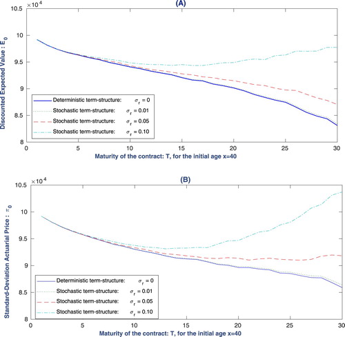
Figure 4, shows the graphical evolution of the price of the participating contract over 30 years of maturities. It represents two different values modeled with the stochastic and deterministic interest rate: (A) for the discounted expected value and (B) for the time-consistent and market-consistent Standard-deviation price. One can observe that for both values with maturities less than T = 5, the randomness of the interest rate (with any level of the interest rate volatility ${\sigma }_r$) is negligible, and further, the difference remains trivial up to T = 10. However, when the maturity increases (T>10), the prices obtained by the stochastic interest rate dominate the price derived by the deterministic interest rate, although the difference between the ${\sigma }_r=0.01$ level and the deterministic rate is still small. The evolution of the value difference for the discounted expected value and Standard-Deviation price with the three levels of ${\sigma }_r$ looks similar, where the interest rate loading for the long-dated contracts with a more volatile interest rate is more drastic, but not so remarkable for the small ${\sigma }_r$. Clearly, with the highly volatile interest rate in the long maturities, the Standard-Deviation price reflects higher interest rate loading as compared to the expected discounted value.

Figure 4. Comparing the effect of the stochastic and deterministic interest rate on the value of the participating contract, simulated with three different levels of the interest rate volatility ${\sigma }_r=\{0.01,0.05,0.1\}$ in the Hull–White model and ${\sigma }_r=0$ for the deterministic interest rate over different maturities $T=\{1,2,\dots ,30\}$. Figure (A): Discounted expected value and figure (B): Time-consistent and market-consistent Standard-Deviation actuarial price. Other parameters set: $A_0=P_0=100$, ${\sigma }_A=15\mathrm{\%}$, ${\sigma }_r=1\mathrm{\%}$, ${\rho }_{A,r}=0.25$, $r_G=2\mathrm{\%}$, $\alpha =0.3$, $\gamma =0.25$, n = 1000, N = 100.

6. Summary and conclusion

In this paper, we focus on the time-consistent and market-consistent valuation of the participating pension contract with a guaranteed annual return and a profit-sharing mechanism. The benefits of the participating contract for a policyholder are a combination of the financial risks such as investment asset, and interest rate risk and actuarial risks such as mortality/longevity. Similar to other insurance products, the liabilities imposed by these products are subject to be valued in a market-consistent setting. Since there is an underlying unhedgeable actuarial risk (mortality/longevity) in the pension contracts, the actuarial value of the contract should be calculated while the financial risk is calculated via a financial pricing framework. If there is any correlation between the actuarial and financial risks to form the final payoff, the price must reflect the possible partial hedging for the actuarial part through financial market dynamics. This can be provided by the time-consistent two-step valuation that is implemented in Salahnejhad & Pelsser (2020).

We assume that the hybrid payoff is a combination of investment on equity, interest rate, and the mortality/longevity risks; for simplicity, the volatility is held constant. We model the investment asset in a Black-Scholes framework with a Geometric Brownian motion (GBM), the Hull–White short rate model for the interest rate risk, and the Lee–Carter model for mortality/longevity risk. We value the discounted payoff with the backward iteration of the two-step actuarial operator over the valuation period. Moreover, the payoff and the overall liability connected to the participating contract is path-dependent through the crediting mechanism. We develop the crediting and profit-sharing from a pure financial mechanism in Grosen & Jorgensen (2000) to a hybrid financial-actuarial mechanism. We introduce a hybrid funding ratio that is multiplied with the updated ratio of the number of survivors at maturity. This gives a more realistic image of the funding evolution where the status of the survivors also plays a role in crediting (or not crediting) interest rate for the policy reserves. The time-consistent two-step operator provides a useful framework to capture the dynamic nature of the hybrid liability we have to value. To numerically calculate the price of the contract, we focus on the finite-difference intervals as the main setup for the discretization of the underlying process and the payoff functions. Note that the payoff is path-dependent and the backward iteration of the operator over the long-term valuation period imposes a massive load on the calculation, especially in higher dimensions. To facilitate more speed and efficiency, we use the Least Square Monte Carlo (LSMC) and regress-later method.

The numerical implementation reflects a diverse result of the time-consistent and market-consistent actuarial prices for the participating contract when different parameters and risk drivers vary. We compare the time-consistent price to other alternative market-consistent prices, like expected value and one-period two-step actuarial value, and represent the risk-loading and the effect of the time-consistency by its risk-premium. We observe that the major part of the actuarial risk-loading is due to the time-consistency risk-premium, and a very small portion of it comes from the one-period loading over the expected value. The results also show that the volatility of the asset return can increase the price. This increase is more significant for the longer maturities and for more liberal profit-sharing policies with a higher distribution ratio and lower requirement for the funding ratio. On the other hand, the volatility of the interest rate dynamics also affects the price. We also studied the effect of the stochastic interest rate by comparing the results provided by different levels of the interest rate volatility and deterministic term structure. The results show that for the short maturities, the time-consistent and the market-consistent actuarial price is not sensitive to the randomness of the interest rate. For the longer maturities, the price is highly sensitive for higher levels of interest rate volatility. However, for small ${\sigma }_r$ in the Hull–White model, the stochastic interest rate does not make a significant difference in the market-consistent price as compared to the deterministic interest rate.

Acknowledgments

The authors are thankful for the helpful comments given by Prof. Dr Jan Dhaene (KU Leuven) on this paper.

Disclosure statement

No potential conflict of interest was reported by the author(s).

Additional information

Funding

The research that produced these results has received funding from the European Union Seventh Framework Programme ([FP7/2007-2013] [FP7/2007-2011]) under grant agreement $n^{\circ }$ 289032; FP7 People: Marie-Curie Actions.

Notes

1 In some countries the market-consistent valuation has become a requirement. For example, in the Netherlands, the Dutch Central Bank (DNB) has imposed such a requirement.

2 If the participating policy includes a surrender option as another stochastic event, where the policyholder may find it more beneficial to sell back the contract than keep it, the policy reserve is strongly path-dependent. In this sense, the contract is similar to an American put option.

3 $P_t+B_t$ constitute the liability side of the balance sheet at time t.

4 α is called the ‘distribution ratio’, the realistic value of which is 20–30%. Additionally, the usual value of γ is around 10–15% (Grosen & Jorgensen 2000).

5 By crediting $r_P\left(t\right)$ at year t, we mean that the interest rate is credited for the period of $(t-1,t)$, and hence is determined at time t−1.

6 This crediting mechanism and the fund evolution is also called the ‘Indexation Ladder’ in the literature.

7 In most countries, this is a real case where those who do not survive until retirement age (or their beneficiaries) cannot benefit from the money they deposit to the fund. The money goes towards compensating the retirement salary of those who live longer.

8 λ is assumed to be constant for simplicity.

9 When $N_x\left(t\right)$ is known, $D_x\left(t\right)$ is always known as well for all $t\le 0$.

10 If $N_x\left(t\right)$ follows a geometric Brownian motion with a constant drift a<0 and volatility, it will be log-normally distributed with mean $N_x\left(0\right)\exp \left(aT\right)$. Accordingly, the technical component (i.e. the ratio of the best-estimate terminal cohort) in Equation (14(14) $\mathrm{H}\mathrm{y}\mathrm{b}\mathrm{r}\mathrm{i}\mathrm{d}\mathrm{f}\mathrm{u}\mathrm{n}\mathrm{d}\mathrm{i}\mathrm{n}\mathrm{g}\mathrm{r}\mathrm{a}\mathrm{t}\mathrm{i}\mathrm{o}=\frac{B{E}_0\left(N_x\left(T\right)\right)A_t}{B{E}_t\left(N_x\left(T\right)\right)P_t}=\frac{\mathbb{E}\left[N_x\left(T\right)\mid N_x\left(0\right)\right]}{\mathbb{E}\left[N_x\left(T\right)\mid N_x\left(t\right)\right]}\times \frac{A_t}{P_t}.$(14) ) can be rewritten as (21) $\begin{array}{rl}\frac{\mathbb{E}\left[N_x\left(T\right)\mid N_x\left(0\right)\right]}{\mathbb{E}\left[N_x\left(T\right)\mid N_x\left(t\right)\right]}& =\frac{N_x\left(0\right)\times e^{a\left(T\right)}}{N_x\left(t\right)\times e^{a(T-t)}}\\ & =\frac{N_x\left(0\right)\times e^{a\left(t\right)}}{N_x\left(t\right)}.\end{array}$(21) The log-normal cohort exhibits a clear interpretation of the technical component, which is the ratio of the expected number of survivors ($N_x\left(0\right)\times e^{a(t-1)}$) to the realized number of survivors ($N_x\left(t\right)$) at time t. Whether the ratio is larger or smaller than one, the hybrid crediting mechanism will act the same as the case of the Poisson cohort and indicate the effect of the local realization of the longevity on the crediting mechanism.

11 As the estimations in Lee-carter model are normally piece-wise annually constant, we focus on annual partitioning over the valuation process. However, the representation is valid for a general case where $[0,T]$ is divided into a partitioning of a shorter or longer sub-intervals with length $\mathrm{\Delta }t$ as $\{0,\mathrm{\Delta }t,2\mathrm{\Delta }t,\dots .,T-\mathrm{\Delta }t,T\}$.

12 According to Pelsser & Stadje (2014), this is valid for all payoffs with factorized form of the financial and actuarial derivatives.

13 In case the actuarial risk ${\kappa }_t$ is independent of the financial risks $A_t$ and $r_t$, the simulation will be reduced to a two-dimensional Brownian motion and an independent one.

14 In particular, for the time-step $(0,1)$, we only need one value out of n realizations as the backward iteration will not go further back.

15 Other values of $N_x\left(T\right)$ are constructed based on the other value of ${\kappa }_t$ or $N_x\left(t\right)$.

16 Note that at t = 1, the technical component, $\frac{{\mathbb{E}}_0\left[N_x\right(T\left)\right]}{{\mathbb{E}}_{t-1}\left[N_x\right(T\left)\right]}$ is equal to one.

17 We prefer $N_x\left(t\right)$ to ${\kappa }_t$ as it captures, by construction, the whole information over the path up to time t and is more informative than ${\kappa }_t$.

18 Accessible from ECB webpage, https://www.ecb.europa.eu/stats/money/yc/html/index.en.html.

19 This means that in the inner step, we omit the loading part of the Standard-Deviation principle and only keep the expectation.

20 As a reminder: this value is by construction time-consistent and market-consistent.

Appendix

The age-specified parameters $a_x$ and $b_x$ estimated in the Lee-Carter model.

Table 4. The age-specified parameters $a_x$ and $b_x$ estimated by the historical population data in The Netherlands through the period 1960–2006.

Age (x)	${\alpha }_x$	${\text{β}}_x$		Age (x)	${\alpha }_x$	${\text{β}}_x$
25	−7.4508	0.0178		66	−3.9628	0.0155
26	−7.4585	0.0177		67	−3.8641	0.0154
27	−7.4502	0.0177		68	−3.7631	0.0149
28	−7.3985	0.0154		69	−3.6715	0.0147
29	−7.3567	0.0160		70	−3.5760	0.0146
30	−7.3149	0.0155		71	−3.4724	0.0142
31	−7.2531	0.0148		72	−3.3705	0.0142
32	−7.2105	0.0151		73	−3.2718	0.0141
33	−7.1309	0.0141		74	−3.1691	0.0142
34	−7.0693	0.0127		75	−3.0687	0.0143
35	−6.9932	0.0145		76	−2.9665	0.0142
36	−6.9091	0.0143		77	−2.8616	0.0139
37	−6.8456	0.0134		78	−2.7608	0.0136
38	−6.7528	0.0146		79	−2.6603	0.0136
39	−6.6510	0.0149		80	−2.5542	0.0135
40	−6.5520	0.0147		81	−2.4469	0.0133
41	−6.4640	0.0140		82	−2.3480	0.0129
42	−6.3461	0.0132		83	−2.2429	0.0125
43	−6.2392	0.0141		84	−2.1383	0.0120
44	−6.1379	0.0134		85	−2.0374	0.0120
45	−6.0342	0.0142		86	−1.9323	0.0112
46	−5.9315	0.0147		87	−1.8338	0.0106
47	−5.8207	0.0134		88	−1.7338	0.0101
48	−5.7208	0.0139		89	−1.6361	0.0093
49	−5.6256	0.0141		90	−1.5468	0.0084
50	−5.5377	0.0139		91	−1.4477	0.0075
51	−5.4308	0.0145		92	−1.3524	0.0076
52	−5.3234	0.0140		93	−1.2624	0.0074
53	−5.2352	0.0156		94	−1.1795	0.0062
54	−5.1363	0.0156		95	−1.0951	0.0057
55	−5.0419	0.0155		96	−1.0075	0.0052
56	−4.9460	0.0158		97	−0.9202	0.0059
57	−4.8399	0.0152		98	−0.8565	0.0039
58	−4.7444	0.0152		99	−0.7810	0.0082
59	−4.6582	0.0162		100	−0.7301	0.0029
60	−4.5483	0.0153
61	−4.4523	0.0149
62	−4.3597	0.0159
63	−4.2547	0.0158
64	−4.1618	0.0153
65	−4.0620	0.0155

References

- Acciaio, B. & Penner, I. (2011). Dynamic convex risk measures. In Di Nunno G., & Øksendal B., editors, Advanced Mathematical Methods for Finance. Berlin: Springer.
- Angelis, P. D., Martire, A. L. & Russo, E. (2014). A bivariate model for evaluating equity-linked policies with surrender option. Scandinavian Actuarial Journal 2016(3), 246–261.
- Artzner, P., Delbaen, F., Eber, J., Heath, D. & Ku, H. (2007). Coherent multiperiod risk adjusted values and Bellman's principle. Annals of Operations Research 152(1), 5–22.
- Bacinello, A. R. (2003). Pricing guaranteed life insurance participating policies with annual premiums and surrender option. North American Actuarial Journal 7, 1–17.
- Bacinello, A. R., Biffis, E. & Millossovich, P. (2010). Regression-based algorithms for life insurance contracts with surrender guarantees. Quantitative Finance 10, 1077–1090.
- Bacinello, A. R., Millossovich, P., Olivieri, A. & Pitacco, E. (2011). Variable annuities: a unifying valuation approach. Insurance: Mathematics and Economics 49, 285–297.
- Barigou, K. & Dhaene, J. (2019). Fair valuation of insurance liabilities via mean-variance hedging in a multi-period setting. Scandinavian Actuarial Journal 2019(2), 163–187.
- Barigou, K., Chen, Z. & Dhaene, J. (2019). Fair dynamic valuation of insurance liabilities: merging actuarial judgement with market- and time-consistency. Insurance: Mathematics and Economics 88, 19–29.
- Bernard, C., Courtois, O. L. & Quittard-Pinon, F. (2005). Market value of life insurance contracts under stochastic interest rates and default risk. Insurance: Mathematics and Economics 36, 499–516.
- Black, F. & Scholes, M. (1973). The pricing of options and corporate liabilities. Journal of Political Economy 81, 637–659.
- Cairns, A., Blake, D. & Dowd, K. (2006). Pricing death: frameworks for the valuation and securitization of mortality risk. Astin Bulletin 36(1), 79–120.
- Cairns, A. J. G., Blake, D., Dowd, K., Coughlan, G. D., Epstein, D., Ong, A. & Balevich, I. (2009). A quantitative comparison of stochastic mortality models using data from England and Wales and the United States. North American Actuarial Journal 13(1), 1–35.
- Cairns, A. J., Blake, D., Dowd, K., Coughlan, G. D., Epstein, D. & Khalaf-Allah, M. (2011). Mortality density forecasts: an analysis of six stochastic mortality models. Insurance: Mathematics and Economics 48, 355–367.
- Carriere, J. (1996). Valuation of the early-exercise price for options using simulations and nonparametric regression. Insurance: Mathematics and Economics 19(1), 19–30.
- Chen, Z., Chen, B. & Dhaene, J. (2020). Fair dynamic valuation of insurance liabilities: a loss averse convex hedging approach. Scandinavian Actuarial Journal 1–27.
- Cheridito, P. & Kupper, M. (2011). Composition of time-consistent dynamic monetary risk measures in discrete time. International Journal of Theoretical and Applied Finance 14.
- Cheridito, P. & Stadje, M. (2009). Time-inconsistency of var and time-consistent alternatives. Finance Research Letters 6(1), 40–46.
- Cheridito, P., Delbaen, F. & Kupper, M. (2006). Dynamic monetary risk measures for bounded discrete-time processes. Electronic Journal of Probability 11(3), 57–106.
- Deelstra, G., Devolder, P., Gnameho, K. & Hieber, P. (2019). Valuation of hybrid financial and actuarial products in life insurance: a universal 3-step method. Available at SSRN: https://ssrn.com/abstract=3307061.
- Delong, L., Dhaene, J. & Barigou, K. (2019a). Fair valuation of insurance liability cash-flow streams in continuous time: applications. ASTIN Bulletin 49(2), 299–333.
- Delong, L., Dhaene, J. & Barigou, K. (2019b). Fair valuation of insurance liability cash-flow streams in continuous time: theory. Insurance: Mathematics and Economics 88, 196–208.
- Dhaene, J., Stassen, B., Barigou, K., Linders, D. & Chen, Z. (2017). Fair valuation of insurance liabilities: merging actuarial judgement and market-consistency. Insurance: Mathematics and Economics 76, 14–27.
- Follmer, H. & Penner, I. (2006). Convex risk measures and the dynamics of their penalty functions. Statistics & Decisions 24(1), 61–96.
- Glasserman, P. (2004). Monte Carlo methods in financial engineering. New York: Springer-Verlag.
- Glasserman, P. & Yu, B. (2004a). Number of paths versus number of basis functions in American option pricing. The Annals of Applied Probability 14(4), 2090–2119.
- Glasserman, P. & Yu, B. (2004b). Pricing american options by simulation: regression now or regression later? In Niederreiter, H., editor, Monte Carlo and Quasi-Monte Carlo methods in scientific computing. Berlin: Springer Verlag. P. 213–226.
- Grosen, A. & Jorgensen, P. L. (2000). Fair valuation of life insurance liabilities: the impact of interest rate guarantees, surrender options, and bonus policies. Insurance: Mathematics and Economics 26, 37–57.
- Hull, J. & White, A. (1996). Using hull-white interest rate trees. The Journal of Derivatives 3(3), 26–36.
- Jobert, A. & Rogers, L. (2008). Valuations and dynamic convex risk measures. Mathematical Finance 18(1), 1–22.
- Kleinow, T. (2009). Valuation and hedging of participating life-insurance policies under management discretion. Insurance: Mathematics and Economics 44, 78–87.
- Kupper, M., Cheridito, P. & Filipovic, D. (2008). Dynamic risk measures, valuations and optimal dividends for insurance. In Mini-workshop: mathematics of solvency. Mathematisches Forschungsinstitut Oberwolfach.
- Lee, R. D. & Carter, L. R. (1992). Modeling and forecasting U.S. mortality. Journal of the American Statistical Association 87(419), 659–671.
- Létourneau, P. & Stentoft, L. (2014). Refining the least squares Monte Carlo method by imposing structure. Quantitative Finance 14, 495–507.
- Li, J. & Szimayer, A. (2014). The effect of policyholders? Rationality on unit-linked life insurance contracts with surrender guarantees. Quantitative Finance 14, 327–342.
- Longstaff, F. A. & Schwartz, E. S. (2001). Valuing American options by simulation: a simple least-squares approach. Review of Financial Studies 14(1), 113–147.
- Madan, D. & Milne, F. (1994). Contingent claims valued and hedged by pricing and investing in a basis. Mathematical Finance 4(3), 223–245.
- Malamud, S., Trubowitz, E. & Wüthrich, M. (2008). Market consistent pricing of insurance products. ASTIN Bulletin 38(2), 483–526.
- Møller, T. (2002). On valuation and risk management at the interface of insurance and finance. British Actuarial Journal 8(4), 787–827.
- Musiela, M. & Zariphopoulou, T. (2004). A valuation algorithm for indifference prices in incomplete markets. Finance and Stochastics 8(3), 399–414.
- Pelsser, A. (2000). Efficient methods for valuing interest rate derivatives. London: Springer Verlag.
- Pelsser, A. & Stadje, M. (2014). Time-consistent and market-consistent evaluations. Mathematical Finance 24(1), 25–65.
- Penner, I. (2007). Dynamic convex risk measures: time consistency, prudence, and sustainability. PhD thesis, Humboldt-Universität zu Berlin.
- Renshaw, A. E. & Haberman, S. (2006). A cohort-based extension to the Lee-Carter model for mortality reduction factors. Insurance: Mathematics and Economics 38, 556–570.
- Roorda, B., Schumacher, J. & Engwerda, J. (2005). Coherent acceptability measures in multiperiod models. Mathematical Finance 15(4), 589–612.
- Rosazza Gianin, E. (2006). Risk measures via g-expectations. Insurance: Mathematics and Economics 39(1), 19–34.
- Salahnejhad, A. & Pelsser, A. (2016). Time-consistent actuarial valuation. Insurance: Mathematics and Economics 66, 97–112.
- Salahnejhad, A. & Pelsser, A. (2020). Market-consistent actuarial valuations with applications to EIOPA risk-margin and time-consistent pricing. Under Review, Graduate School of Business and Economics, Maastricht University.
- Shreve, S. E. (2010). Stochastic calculus for finance II, continuous-time models. New York: Springer Finance.
- Stadje, M. (2010). Extending dynamic convex risk measures from discrete time to continuous time: a convergence approach. Insurance: Mathematics and Economics 47(3), 391–404.
- Stentoft, L. (2004). Convergence of the least squares Monte Carlo approach to American option valuation. Management Science 50, 1193–1203.
- Tanskanen, A. J. & Lukkarinen, J. (2003). Fair valuation of path-dependent participating life insurance contracts. Insurance: Mathematics and Economics 33, 595–609.
- Zaglauer, K. & Bauer, D. (2008). Risk-neutral valuation of participating life insurance contracts in a stochastic interest rate environment. Insurance: Mathematics and Economics 43, 29–40.
Appendix
The age-specified parameters and
estimated in the Lee-Carter model.