Cramér–Lundberg asymptotics for spectrally positive Markov additive processes

Abstract

This paper studies the Cramér–Lundberg asymptotics of the ruin probability for a model in which the reserve level process is described by a spectrally-positive light-tailed Markov additive process. By applying a change-of-measure technique in combination with elements from Wiener-Hopf theory, the exact asymptotics of the ruin probability are expressed in terms of the model primitives. In addition a simulation algorithm of generalized Siegmund type is presented, under which the returned estimate of the ruin probability has bounded relative error. Numerical experiments show that, compared to direct estimation, this algorithm greatly reduces the number of runs required to achieve an estimate with a given accuracy. The experiments also reveal that our asymptotic results provide a good approximation of the ruin probability even for relatively small initial surplus levels.

Keywords:

• Cramér–Lundberg asymptotics
• ruin probability
• Lévy process
• Markov additive process
• running maximum
• overshoot

1. Introduction

Primarily motivated by applications in insurance risk, much attention has been directed to evaluating ruin probabilities (Asmussen & Albrecher 2010). In this context, one typically assumes that the driving net cumulative claim process $X(\cdot )$ is of Lévy type (or a subclass thereof, such as the compound Poisson process). With the insurance firm's initial surplus being u, one is mainly interested in computing the probability $p(u)$ of the surplus level process $u-X(\cdot )$ dropping below 0. If this is beyond reach, which is often the case, one may settle for the (exact) tail asymptotics, the goal being to identify an explicit function $\overline{p}(u)$ such that $p(u)/\overline{p}(u)\to 1$ as $u\to \mathrm{\infty }$.

Research into such exact asymptotics goes back about a century. In the regime that the driving Lévy process is of compound Poisson type, and in case the claim size distribution is light-tailed, the classical Cramér-Lundberg asymptotics entail that $p(u)$ decays, for u large, like $\overline{p}(u)=\alpha {\mathrm{e}}^{-{\theta }^{\star }u}$ for positive constants α and ${\theta }^{\star }$ (where the decay rate ${\theta }^{\star }$ solves the so-called Lundberg equation). In the analysis one often relies on a duality with the stationary workload in the M/G/1 queue; see e.g. (Asmussen & Albrecher 2010, Ch. IV.2) and (Debicki & Mandjes 2015). Where in the literature the focus lies on finding the exact tail asymptotics for spectrally-positive (i.e. having only positive jumps) light-tailed Lévy processes, Bertoin & Doney (1994) derive such asymptotics for their spectrally two-sided counterpart (i.e. having jumps in both directions).

A natural extension of the above body of work concerns exact tail asymptotics of ruin probabilities in the context of Markov additive processes (MAPs) (Çinlar 1972, Neveu 1961). These are essentially Markov modulated Lévy processes with in addition jumps at transition epochs of the modulating process (also often referred to as background process). More explicitly, a MAP $Y(\cdot )$ behaves as the Lévy process $X_i(\cdot )$ when its Markovian background chain $J(\cdot )$ (evolving independently of the process $Y(\cdot )$ itself) is in state i, and may in addition have a jump at each transition of $J(\cdot )$. Because of the state changes, MAPs are particularly suitable for modeling real-world processes of which the behavior changes over time.

A main objective of this paper is to establish the exact tail asymptotics of the ruin probability $p(u)$ when the driving process is a spectrally-positive light-tailed MAP. We find that these asymptotics are of Cramér-Lundberg type, i.e. they are of the form $\overline{p}(u)=\alpha {\mathrm{e}}^{-{\theta }^{\star }u}$ for positive α and ${\theta }^{\star }$. The present paper complements our recent work (van Kreveld et al. 2022) and its predecessors, such as D'Auria et al. (2010), Dieker & Mandjes (2011), and Ivanovs (2011), which succeeded in identifying the Laplace transform of $p(u)$ for spectrally one-sided MAPs. With the expressions found there, one could in principle try to perform Laplace inversion in order to obtain numerical values for $p(u)$, but a complication is that these become inaccurate in the regime that ruin is rare. The findings of the present paper remedy this issue: we provide an asymptotic expansion that becomes increasingly accurate as u grows.

Cramér-Lundberg asymptotics have been studied for various kinds of specific MAPs. Without providing an exhaustive overview, we discuss a few relevant contributions. Siegl & Tichy (1999) consider a compound Poisson process with dividend barrier and two possible claim frequencies governed by a two-state Markov chain. In Jasiulewicz (2001) a model is analyzed with the premium rate depending continuously on the reserve level and the Markov-modulated claim frequency. More general MAPs of compound Poisson type are studied with constant premium rate (Miyazawa 2002) or constant claim frequency (Yin et al. 2006). The case where all components of the compound Poisson process are allowed to change with the background chain is considered by Zhu & Yang (2009). Typically, for the case that the driving process is of MAP type, the prefactor α is characterized relatively implicitly; see e.g. (Asmussen & Albrecher 2010, Theorem VII.3.7), where α is expressed in terms of random quantities at a stopping time under an alternative probability measure. An exception to this is the work of Miyazawa (2004) on the Cramér-Lundberg asymptotics of a Markov-modulated compound Poisson process including jumps at transition epochs. By considering a ladder-height approach, that work determines an explicit expression for the prefactor α for this model.

In detail, the contributions of this paper are the following:

°

In the first place, we succeed in establishing exact asymptotics $\overline{p}(u)=\alpha {\mathrm{e}}^{-{\theta }^{\star }u}$ for the ruin probability $p(u)$ in the model where the net cumulative claim process is represented by a spectrally-positive MAP $Y(\cdot )$ with light-tailed claim sizes and negative drift (such that $p(u)\to 0$ as $u\to \mathrm{\infty }$). Through a delicate analysis of the overshoot of $Y(\cdot )$ over level u (under a specific alternative probability measure), we manage to express the constants α and ${\theta }^{\star }$ in terms of the model primitives. By lower bounding the overshoot by 0 we obtain, as a by-product, a version of the Lundberg inequality for light-tailed spectrally-positive MAPs.

°

Secondly, we show that the ruin probability $p(u)$ can be efficiently computed by simulation; this is particularly useful in the regime that ruin is rare, in which direct simulation would be extremely time-consuming. To this end, we construct a generalized version of Siegmund's algorithm (Asmussen & Glynn 2007, Ch. VI.2), which amounts to performing importance sampling using the alternative measure that we identified when establishing the exact asymptotics. The resulting estimator can be considered optimal, in that we succeed in proving that it has bounded relative error. Numerical experiments reveal that the number of runs required to obtain an estimate with a given precision (i.e. the ratio of the width of the confidence interval and the estimate) is essentially constant in u; this is a huge improvement over direct simulation, under which this number of runs roughly grows as ${\mathrm{e}}^{{\theta }^{\star }u}$. The experiments also show that $\overline{p}(u)=\alpha {\mathrm{e}}^{-{\theta }^{\star }u}$ is an accurate approximation of the ruin probability, even for relatively small initial surplus levels u.

A crucial idea underlying our analysis is the observation that in order to identify whether the spectrally-positive MAP $Y(\cdot )$ has crossed level u, it is sufficient to monitor only the maxima of $Y(\cdot )$ between every two successive transition epochs of the background process; in other words, it is not needed to monitor $Y(\cdot )$ continuously in time. The resulting embedded process turns out to be conceptually substantially simpler than the original one. When deriving the exact asymptotics via the embedded process, two steps play a key role at the technical level. (i) The first concerns the introduction of a specific new probability measure $\mathbb{Q}$ under which the net cumulative claim process $Y(\cdot )$ has a positive drift, so that ruin occurs almost surely; see for instance (Asmussen & Albrecher 2010, Ch. VII.3). The main idea is then to write $p(u)$ in terms of the likelihood ratio of a path to ruin under the original measure $\mathbb{P}$, relative to the new measure $\mathbb{Q}$. This reasoning leads to an expression for $p(u)$ in terms of the overshoot of $Y(\cdot )$ over u under $\mathbb{Q}$. (ii) In the second step, which combines application of the Wiener-Hopf decomposition with a result (Ivanovs et al. 2010) on the number of zeroes of the matrix-exponent corresponding to the MAP under consideration, this overshoot is analyzed in further detail (in the regime that $u\to \mathrm{\infty }$).

The outline of this paper is as follows. Section 2 defines our MAP $Y(\cdot )$, introduces the ruin probability $p(u)$, and highlights a number of relevant preliminary results. The change-of-measure argument is carried out in Section 3, which leads, as mentioned above, to an expression for $p(u)$ in terms of the overshoot of $Y(\cdot )$ over u under $\mathbb{Q}$. As an intermediate step towards the identification of the exact asymptotics of $p(u)$, the purpose of Section 4 is to find the transform of the overshoot distribution under $\mathbb{Q}$. As it turns out, this overshoot transform can be expressed in terms of the solution to a set of linear equations. Combining the above findings, in Section 5 the exact asymptotics of the ruin probability are derived (i.e. the constants α and ${\theta }^{\star }$ in $\overline{p}(u)=\alpha {\mathrm{e}}^{-{\theta }^{\star }u}$ are identified). A simulation algorithm of generalized Siegmund type, enabling fast estimation of $p(u)$, is given in Section 6. In addition, we give a proof for its bounded relative error, making the algorithm particularly useful in the rare-event regime. Finally, Section 7 presents the output of simulation experiments that provide an indication of the achievable speedup, as well as of the accuracy of the approximation $p(u)\approx \overline{p}(u)$.

2. Model and preliminaries

In this section, we first describe in detail the model that we consider in this paper and introduce the corresponding notation. We then discuss the Wiener-Hopf decomposition for spectrally-positive Lévy processes and the result concerning the number of singularities of a spectrally one-sided MAP. Finally, we briefly outline the approach that we will follow in later sections to establish the exact asymptotics. The model, notation and preliminaries strongly resemble those featuring in van Kreveld et al. (2022), save for a few specific aspects (e.g. the restriction to spectrally-positive processes, the background process being irreducible, and a slightly different version of Proposition 2.2).

2.1. Model

We start by defining our model. Let the background process $J(\cdot )\equiv (J(t){)}_{t⩾0}$ be an irreducible continuous-time Markov chain with state space $\{1,\dots ,d\}$ for d>1. The corresponding transition rate matrix (or: generator matrix) is given by $Q=(q_{\mathrm{ij}}{)}_{i,j=1}^d$, with $q_i:=-q_{\mathrm{ii}}>0$, having invariant probability distribution $\mathit{\pi }=({\pi }_1,\dots ,{\pi }_d)$. Associated with every state i, let $X_i(\cdot )\equiv (X_i(t){)}_{t⩾0}$ be a spectrally-positive Lévy process, evolving independently of $J(\cdot )$. Informally, when $J(t)=i$, the process $Y(\cdot )\equiv (Y(t){)}_{t⩾0}$ behaves as the Lévy process $X_i(\cdot )$. Additionally, the process is allowed to have non-negative jumps at transition epochs of the background process. For that purpose, let $(L_{\mathrm{ij}}^n{)}_{n\in \mathbb{N}}$ (with $i,j\in \{1,\dots ,d\}$ such that $i\ne j$) be a sequence of independent copies of the non-negative random variable $L_{\mathrm{ij}}$, independent of anything else, representing the jumps at the epochs that $J(\cdot )$ jumps from state i to state j.

The MAP $Y(\cdot )$ can be formally defined as follows. Let $t_n$ denote the time of the nth transition of the background chain. If $J(0)=i$, we have that $Y(t)=X_i(t)$ for $t\in [0,t_1)$, and, if the transition at $t_n$ is from (say) i to j (where $i\ne j$), then $Y(t):=Y(t_n-)+L_{\mathrm{ij}}^n+(X_j(t)-X_j(t_n)),$ where $t\in [t_n,t_{n+1})$ and $n\in \mathbb{N}$. We say that the thus constructed process $Y(\cdot )$ is a spectrally-positive Markov additive process (MAP).

2.2. Notation and objective

Each of the spectrally-positive Lévy processes $X_i(\cdot )$ is defined through its Laplace exponent ${\phi }_i(\cdot )$: ${\phi }_i(\alpha ):=\log \mathbb{E}{\mathrm{e}}^{-\alpha X_i(1)}$ for $\alpha ⩾0$, where the corresponding right inverse is denoted by ${\psi }_i(\cdot )$. In the sequel, $M(\alpha )=(m_{\mathrm{ij}}(\alpha ){)}_{i,j=1,\dots ,d}$ denotes the matrix with entries (1) $m_{\mathrm{ij}}(\alpha ):=q_{\mathrm{ij}}{\lambda }_{\mathrm{ij}}(\alpha )+{\phi }_i(\alpha ){\mathbf{1}}_{\{i=j\}},$(1) with ${\lambda }_{\mathrm{ij}}(\alpha ):=\mathbb{E}{\mathrm{e}}^{-\alpha L_{\mathrm{ij}}}$. The matrix exponent $M(\alpha )$ can be seen as the MAP counterpart of the Laplace exponent.

The aim of this paper is to identify the tail asymptotics of the maximum of the MAP conditional on the initial background state being $i\in \{1,\dots ,d\}$. That is, with $p_i(u):=\mathbb{P}(\underset{s⩾0}{max}Y(s)⩾u|J(0)=i),$ we wish to find an explicit function ${\overline{p}}_i(u)$ such that $p_i(u)/{\overline{p}}_i(u)\to 1$ as $u\to \mathrm{\infty }$. We say that ${\overline{p}}_i(u)$ are the exact asymptotics of $p_i(u)$. We throughout assume that $Y(\cdot )$ has a negative drift, i.e. (2) $\mu :=\sum _{i=1}^d{\pi }_i\mathbb{E}{X}_i(1)+\sum _{i=1}^d\sum _{k\ne i}{\pi }_i{q}_{\mathrm{ik}}\mathbb{E}{L}_{\mathrm{ij}}<0,$(2) such that exceeding u is increasingly rare as $u\to \mathrm{\infty }$; in the actuarial literature, this condition is known as the net profit condition. The focus is on a light-tailed spectrally-positive MAP, under which $p_i(u)$ decays effectively exponentially. We provide a more precise description of what we mean by the MAP being light-tailed in Section 3.

2.3. Preliminaries

Two important results play a crucial role in the derivation of the exact asymptotics of $p_i(u)$: the Wiener-Hopf decomposition for spectrally-positive Lévy processes and a fundamental result on the zeroes of $\det M(\alpha )$.

The Wiener-Hopf decomposition states that the value of any Lévy process at an exponentially distributed epoch can be written as the difference between two independent non-negative random quantities. In the context of this paper, we specifically consider the case of a spectrally-positive Lévy process $(X(t){)}_{t⩾0}$ with Laplace exponent $\phi (\cdot )$ and corresponding right inverse $\psi (\cdot )$. Denote by $(\overline{X}(t){)}_{t⩾0}$ the running maximum process associated with $(X(t){)}_{t⩾0}$, and by $(\underset{\_}{X}(t){)}_{t⩾0}$ the corresponding running minimum process. In the sequel, $T_{\nu }$ is an exponentially distributed random variable with mean ${\nu }^{-1}$, assumed independent of anything else.

Proposition 2.1

Wiener–Hopf decomposition

Let $(X(t){)}_{t⩾0}$ be a spectrally-positive Lévy process. Then $X(T_{\nu })$ can be decomposed as the sum of the two independent quantities $\overline{X}(T_{\nu })$ and $X(T_{\nu })-\overline{X}(T_{\nu })$. Moreover, $X(T_{\nu })-\overline{X}(T_{\nu })$ has the same distribution as $\underset{\_}{X}(T_{\nu })$ which is distributed as $-T_{\psi (\nu )}$. In addition, $\mathbb{E}\left({\mathrm{e}}^{-\gamma \overline{X}(T_{\nu })}\right)=\frac{\nu }{\nu -\phi (\gamma )}(1-\frac{\gamma }{\psi (\nu )}).$

For a detailed account, see e.g. Kyprianou (2006, Ch. 6).

The second result concerns a characterization of the zeroes of the determinant of the matrix exponent $M(\alpha )$ of a spectrally-positive MAP. In this result an important role is played by the Lévy processes $X_i(\cdot )$ that are (almost surely) increasing (also referred to as subordinators). Let $S^{\uparrow }$ denote the set of background states corresponding to these subordinators. The following result is (Ivanovs et al. 2010, Theorem 1).

Proposition 2.2

Let $(Y(t){)}_{t⩾0}$ be a spectrally-positive MAP, and let the underlying background process $(J(t){)}_{t⩾0}$ be irreducible. Then the equation $detM(\gamma )=0$ has $d-|S^{\uparrow }|-{\mathbb{1}}_{\mu ⩽0}$ solutions in $\mathbb{C}$ with positive real part. Additionally, it holds that $detM(0)=0$.

2.4. Approach

We conclude this section with a short account of the approach followed in the derivation of the exact asymptotics, as covered by Sections 3–5. The MAP itself being a rather involved object, we work with a more manageable embedded version. This embedded process is constructed in such a way that the event of the MAP exceeding u is equivalent to the event of the embedded process exceeding u. More specifically, throughout this paper we restrict ourselves, similar to the approach followed in van Kreveld et al. (2022), to the value of $Y(\cdot )$ at only three types of time points. In the interval between two transitions of the background process we record the value of $Y(\cdot )$

1. at the start of the interval (right after the jump at transition epoch, that is),

2. at the epoch that the maximum value (within the interval) is achieved, and

3. at the end of the interval (right before the jump at transition epoch, that is).

It can be seen that in order to verify whether $Y(\cdot )$ exceeds u we can restrict ourselves to the values of the MAP at epochs of type (ii). The increments of the MAP between the embedded time points are relatively straightforward to deal with, as a consequence of Proposition 2.1.

In Section 3, we work with the above embedding to find an alternative expression for the ruin probability under an alternative measure $\mathbb{Q}$. Concretely, we succeed in expressing $p_i(u)$ in terms of the overshoot of $Y(\cdot )$ over level u under $\mathbb{Q}$. This overshoot is then analyzed in Section 4, which eventually leads to the exact asymptotics of $p_i(u)$ in Section 5.

3. Change of measure

In this section, we derive an alternative expression for the ruin probability $p_i(u)$ by applying a change of measure. The derivation consists of the following four steps:

1. constructing a system of equations for finding the positive solution to the so-called Lundberg equation, providing the candidate for the exponential decay rate ${\theta }^{\star }$ appearing in the exact asymptotics of $p_i(u)$ (where we remark that we show later that ${\theta }^{\star }$ is independent of the initial state i);

2. defining an embedding of the MAP $Y(\cdot )$, based on the time points of type (i), (ii) and (iii) that were introduced in Section 2.2;

3. defining an alternative probability measure $\mathbb{Q}$, also corresponding to a MAP, but with different driving Lévy processes, a different Markovian background process, and jumps at transition epochs having different distributions;

4. calculating the likelihood ratio of the actual probability measure $\mathbb{P}$ with respect to the new probability measure $\mathbb{Q}$, through which we find a compact expression for our target probability $p_i(u)$.

The compact expression for $p_i(u)$ provides us with an explicit (exponentially decaying) bound on $p_i(u)$, uniformly in $u⩾0$. More importantly, however, it also eventually allows us to evaluate the exact asymptotics of $p_i(u)$, as shown in Sections 4 and 5.

3.1. Step 1: the Lundberg equation

The Lundberg equation, which yields the candidate for the exponential decay rate ${\theta }^{\star }$ appearing in the exact asymptotics of $p_i(u)$, involves the increment of the MAP between two consecutive epochs that the background state changes to an (arbitrarily chosen) reference state $i_0\in \{1,\dots ,d\}$. The goal of Step 1 is to quantify the moment generating function of this increment, providing the solution to the Lundberg equation.

Denote, for $i=1,\dots ,d$, by $(V_i^n{)}_{n\in \mathbb{N}}$ a sequence of independent random variables being distributed as the generic random variable $V_i:=\overline{X_i}(T_{q_i})$ (in words: the maximum of the spectrally-positive Lévy process $X_i(\cdot )$ over an exponentially distributed time with mean $q_i^{-1}$). Also, denote by $(W_i^n{)}_{n\in \mathbb{N}}$ a sequence of independent random variables distributed as the generic random variable $W_i:=-\underset{\_}{X_i}(T_{q_i})$ (in words: minus the minimum of the spectrally-positive Lévy process $X_i(\cdot )$ over an exponentially distributed time with mean $q_i^{-1}$); recall from Proposition 2.1 that $W_i$ is exponentially distributed with parameter ${\delta }_i:={\psi }_i(q_i)$. Let the resulting $2d$ sequences be independent. Due to Proposition 2.1, the Laplace-Stieltjes transforms of these random variables are given by $\begin{array}{rl}{v}_i(\alpha )& :=\mathbb{E}{\mathrm{e}}^{-\alpha V_i}={\int }_0^{\mathrm{\infty }}{\mathrm{e}}^{-\mathrm{\alpha x}}{f}_i^{(\mathbb{P})}(x)\mathrm{d}x=\frac{q_i}{q_i-{\phi }_i(\alpha )}(1-\frac{\alpha }{{\delta }_i}),\\ w_i(\alpha )& :=\mathbb{E}{\mathrm{e}}^{-\alpha W_i}={\int }_0^{\mathrm{\infty }}{\mathrm{e}}^{-\mathrm{\alpha x}}{g}_i^{(\mathbb{P})}(x)\mathrm{d}x=\frac{{\delta }_i}{{\delta }_i+\alpha },\end{array}$ with $f_i^{(\mathbb{P})}(\cdot )$ the density of $V_i$ and $g_i^{(\mathbb{P})}(\cdot )$ the density of $W_i$ (for ease assumed to exist), both under the original measure $\mathbb{P}$. Below, we will use the notation $h_{\mathrm{ij}}^{(\mathbb{P})}(\cdot )$ for the density of $L_{\mathrm{ij}}$ under $\mathbb{P}$.

Now fix a reference state $i_0\in \{1,\dots ,d\}$, and define by U the increment of $Y(\cdot )$ between two subsequent visits of the background process to this state $i_0$. That is, if $t_n$ and $t_m$ are two subsequent times that the background chain enters state $i_0$, then U is distributed as $Y(t_m)-Y(t_n)$. We assume that we are in the light-tailed regime, in the sense that the Lundberg equation $\tilde{u}(\theta ):=\mathbb{E}{\mathrm{e}}^{\mathrm{\theta U}}=1$ has a positive solution, say ${\theta }^{\star }$; in the literature, $\tilde{u}(\theta )$ is referred to as the moment generating function (mgf) of the random variable U.

Four remarks are in place now. In the first place, note that our assumption is similar to that of (Debicki & Mandjes 2015, Section 8.1) for the Lévy case (i.e. covering the situation without any background process). In the second place, the fact that the Lundberg equation has a positive solution implies that the jumps $L_{\mathrm{ij}}$ have a finite mgf in an open interval around the origin, and that the same holds for the mgfs of the possible upward jumps of the Lévy processes $X_i(\cdot )$. It is for this reason that we call the driving MAP $Y(\cdot )$ light-tailed. In the third place, since $\tilde{u}(0)=1$, ${\tilde{u}}^{\prime }(0)<0$ and $\underset{\theta \to \mathrm{\infty }}{lim}\tilde{u}(\theta )=\mathrm{\infty }$, the existence of a positive solution to $\tilde{u}(\theta )=1$ excludes cases in which $\tilde{u}$ ‘jumps over 1’ at some $\theta >0$. In the fourth place, we note that it may seem that ${\theta }^{\star }$ depends on the reference state $i_0$ chosen. Below, however, we argue that the choice of $i_0$ does not affect the value of ${\theta }^{\star }$.

Next, we show that we can express the root ${\theta }^{\star }$ in terms of a generalized eigensystem. Let $y_j\equiv y_j(\theta )$, for $j\ne i_0$, be the moment generating function of the increment of $Y(\cdot )$, with the background process starting in state j, before the background process reaches the reference state $i_0$. To derive a system of equations, consider an increment of $Y(\cdot )$ in an interval of the type $(t_n,t_{n+1}]$, that is, an interval between two successive transition epochs of the background process $J(\cdot )$. By Proposition 2.1, we know that such an increment can be written as the sum of three independent variables: the maximum of the corresponding Lévy process in this interval, the decrease after this maximum, and the jump at the transition epoch. In terms of moment generating functions this leads to the equations $\tilde{u}(\theta )=y_{i_0}=v_{i_0}(-\theta )w_{i_0}(\theta )\sum _{j\ne i_0}\frac{q_{i_{0}j}}{q_{i_0}}{\lambda }_{i_{0}j}(-\theta )y_j,$ and, for $j\ne i_0$, (3) $y_j=v_j(-\theta )w_j(\theta )(\frac{q_{j{i}_0}}{q_j}{\lambda }_{j{i}_0}(-\theta )+\sum _{k\ne j,i_0}\frac{q_{\mathrm{jk}}}{q_j}{\lambda }_{\mathrm{jk}}(-\theta )y_k).$(3) Then we equate $\tilde{u}(\theta )$ to 1, in order to find ${\theta }^{\star }$. We thus end up with the following system of equations: for $i=1,\dots ,d$, (4) $q_i{y}_i=v_i(-\theta )w_i(\theta )\sum _{j\ne i}{q}_{\mathrm{ij}}{\lambda }_{\mathrm{ij}}(-\theta )y_j,$(4) with $y_{i_0}=1$. Note that if $\mathit{y}$ solves this system of equations, then so does $c\cdot \mathit{y}$ for any c, implying that the solution ${\theta }^{\star }$ does not depend on the reference state $i_0$. It also means that $\mathit{y}$ is unique up to a multiplication by a factor, so that ratios of the type $y_i/y_j$ are uniquely determined. Due to the fact that the components of the vector $\mathit{y}=\mathit{y}({\theta }^{\star })$ can be interpreted as moment generating functions, we conclude that $\mathit{y}$ is necessarily componentwise positive. Below we will use the eigenvalue/eigenvector pair $({\theta }^{\star },\mathit{y})$ when defining the alternative measure $\mathbb{Q}$.

3.2. Step 2: the embedding

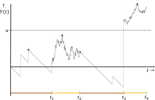
The idea is to embed the process $Y(\cdot )$ into a simpler process that still contains all information based on which it can be determined whether it exceeds level u. To this end, observe that it suffices to consider only the values of $Y(\cdot )$ that correspond to maxima between transitions of the background process. This observation is visualized in Figure 1; the maxima between transition epochs (i.e. the dots) give all information that is needed to verify whether level u is ever crossed.

Figure 1. Example of a MAP with two background states, with dots representing the embedded process $(S_n{)}_n$. That is, the dots represent the maxima over the intervals $[t_n,t_{n+1})$ for $n\in \mathbb{N}$.

Define the embedded process $(S_n{)}_n$ by $\begin{array}{rl}{S}_0& :=V_{K_0}^0,\\ S_n& :=S_{n-1}-W_{K_{n-1}}^n+L_{K_{n-1},K_n}^n+V_{K_n}^n,n=1,2,\dots ,\end{array}$ with $K_0:=J(0)$ and $K_n:=J(t_n)$ denoting the state of the background process right after the nth transition of the background process.

As discussed above, and appealing to Proposition 2.1 to justify the independence between the sequences $(V_i^n{)}_{n\in \mathbb{N}}$ and $(W_i^n{)}_{n\in \mathbb{N}}$, we can rewrite the ruin probability $p_i(u)$ in terms of the embedded process $(S_n{)}_n$, as follows: $p_i(u)=\mathbb{P}(\mathrm{\exists n}\in {\mathbb{N}}_0:S_n⩾u|K_0=i).$

3.3. Step 3: construction of the alternative probability measure

To evaluate the ruin probability in the regime that $u\to \mathrm{\infty }$, we work with a change of measure. Particularly, we set up the alternative probability measure $\mathbb{Q}$ (to be defined below), under which the process is still a MAP, but now has positive drift. The goal is to evaluate $p_i(u)$ where the path of $(S_n{)}_n$ is sampled under $\mathbb{Q}$. The measure $\mathbb{Q}$ is an exponentially twisted version of $\mathbb{P}$, in that (5) ${\mathbb{E}}_{\mathbb{Q}}{\mathrm{e}}^{\mathrm{\theta U}}=\mathbb{E}{\mathrm{e}}^{(\theta +{\theta }^{\star })U}=\tilde{u}(\theta +{\theta }^{\star })$(5) (where a more descriptive definition will be given below). This change of measure has been employed for the random walk (Asmussen 2003, Chapter XIII) and Lévy (Debicki & Mandjes 2015, Section VIII.1) cases.

From $\tilde{u}(\cdot )$ being convex, ${\tilde{u}}^{\prime }(0)<0$ (due to (2(2) $\mu :=\sum _{i=1}^d{\pi }_i\mathbb{E}{X}_i(1)+\sum _{i=1}^d\sum _{k\ne i}{\pi }_i{q}_{\mathrm{ik}}\mathbb{E}{L}_{\mathrm{ij}}<0,$(2) )) and $\tilde{u}(0)=\tilde{u}({\theta }^{\star })=1$, it follows that ${\tilde{u}}^{\prime }({\theta }^{\star })>0$, which means that under the new measure $\mathbb{Q}$ the drift of $(S_n{)}_n$ has become positive, so that u is eventually exceeded almost surely under $\mathbb{Q}$. As an aside, we also note that if state i corresponds to a subordinator process $X_i(\cdot )$ under $\mathbb{P}$, then the same applies under $\mathbb{Q}$ (and vice versa).

Let $\ell \equiv \ell (S)$ be the appropriate likelihood ratio (or Radon-Nikodym derivative), which records the likelihood of the path of $(S_n{)}_n$ under $\mathbb{P}$ relative to $\mathbb{Q}$ (until $(S_n{)}_n$ exceeds u, that is). Then we have the following standard equality translating the likelihood of outcomes under $\mathbb{Q}$ into those under $\mathbb{P}$: $p_i(u)=\mathbb{E}(1\{\mathrm{\exists n}\in {\mathbb{N}}_0:S_n⩾u\}|K_0=i)={\mathbb{E}}_{\mathbb{Q}}(\ell (S)1\{\mathrm{\exists n}\in {\mathbb{N}}_0:S_n⩾u\}|K_0=i).$ An important benefit of working with $\mathbb{Q}$ is that under this measure, the event in the indicator function has probability 1 due to the positive drift, whereas under $\mathbb{P}$ the same probability vanishes as u becomes large; as a consequence, (6) $p_i(u)={\mathbb{E}}_{\mathbb{Q}}(\ell (S)|K_0=i).$(6) It is noted that by many other definitions of $\mathbb{Q}$ we could have achieved a positive drift, and thus the validity of (6(6) $p_i(u)={\mathbb{E}}_{\mathbb{Q}}(\ell (S)|K_0=i).$(6) ). The crucial feature of our specific alternative measure, as given in (5(5) ${\mathbb{E}}_{\mathbb{Q}}{\mathrm{e}}^{\mathrm{\theta U}}=\mathbb{E}{\mathrm{e}}^{(\theta +{\theta }^{\star })U}=\tilde{u}(\theta +{\theta }^{\star })$(5) ), however, is that for this $\mathbb{Q}$ the likelihood ratio ℓ takes a simple form, as we will show below.

The alternative measure $\mathbb{Q}$, in an abstract sense defined via (5(5) ${\mathbb{E}}_{\mathbb{Q}}{\mathrm{e}}^{\mathrm{\theta U}}=\mathbb{E}{\mathrm{e}}^{(\theta +{\theta }^{\star })U}=\tilde{u}(\theta +{\theta }^{\star })$(5) ), is concretely described as follows. Under $\mathbb{Q}$, the distributions of $(V_i^n{)}_n$ and $(W_i^n{)}_n$ are characterized through the densities $f_i^{(\mathbb{Q})}(x)=f_i^{(\mathbb{P})}(x)\frac{{\mathrm{e}}^{{\theta }^{\star }x}}{v_i(-{\theta }^{\star })},g_i^{(\mathbb{Q})}(x)=g_i^{(\mathbb{P})}(x)\frac{{\mathrm{e}}^{-{\theta }^{\star }x}}{w_i({\theta }^{\star })},$ respectively, for $i=1,\dots ,n$ and x>0. Note that this means that the Laplace-Stieltjes transform of the $(V_i^n{)}_n$ under $\mathbb{Q}$ becomes $v_i^{(\mathbb{Q})}(\alpha )=\frac{v_i(\alpha -{\theta }^{\star })}{v_i(-{\theta }^{\star })}$ and that under $\mathbb{Q}$ the $(W_i^n{)}_n$ are exponentially distributed with parameter ${\delta }_i^{(\mathbb{Q})}:={\delta }_i+{\theta }^{\star }.$ In addition, the $(L_{\mathrm{ij}}^n{)}_n$ under $\mathbb{Q}$ have density $h_{\mathrm{ij}}^{(\mathbb{Q})}(x)=h_{\mathrm{ij}}^{(\mathbb{P})}(x)\frac{{\mathrm{e}}^{{\theta }^{\star }}x}{{\lambda }_{\mathrm{ij}}(-{\theta }^{\star })},$ where, in the same way as above, the corresponding Laplace-Stieltjes transform can be verified to be ${\lambda }_{\mathrm{ij}}^{(\mathbb{Q})}(\alpha )={\lambda }_{\mathrm{ij}}(\alpha -{\theta }^{\star })/{\lambda }_{\mathrm{ij}}(-{\theta }^{\star })$.

Now that we have defined the driving Lévy processes and the jumps at transition epochs under $\mathbb{Q}$, we conclude by considering the transition rates of the background process under $\mathbb{Q}$. For $i\ne j$ these become $q_{\mathrm{ij}}^{(\mathbb{Q})}=q_{\mathrm{ij}}{\lambda }_{\mathrm{ij}}(-{\theta }^{\star })\frac{y_j}{y_i}.$ It is readily verified that this choice implies that the diagonal elements of the transition rate matrix under $\mathbb{Q}$ are $q_{\mathrm{ii}}^{(\mathbb{Q})}=-\sum _{j\ne i}{q}_{\mathrm{ij}}^{(\mathbb{Q})}=-\sum _{j\ne i}{q}_{\mathrm{ij}}{\lambda }_{\mathrm{ij}}(-{\theta }^{\star })\frac{y_j}{y_i}=-q_i\frac{1}{v_i(-{\theta }^{\star })w_i({\theta }^{\star })},$ where the last equality is by virtue of (4(4) $q_i{y}_i=v_i(-\theta )w_i(\theta )\sum _{j\ne i}{q}_{\mathrm{ij}}{\lambda }_{\mathrm{ij}}(-\theta )y_j,$(4) ).

3.4. Step 4: the likelihood ratio

The next step is to evaluate the likelihood ratio $\ell (S)$ on a path such that $(S_n{)}_n$ reaches u, which is equal to $p_i(u)$ by (6(6) $p_i(u)={\mathbb{E}}_{\mathbb{Q}}(\ell (S)|K_0=i).$(6) ). Let $N\equiv N(u)$ denote the first n for which $S_n⩾u$ (which is under the new measure $\mathbb{Q}$ finite almost surely). Then $\ell \equiv \ell (S)$ can be written as the product of the following four factors corresponding to the elements of the MAP that change under $\mathbb{Q}$: the maxima and minima of the underlying Lévy processes between two transition epochs, the jumps at transition epochs and the transition rates of the background chain.

°	In the first place there is the contribution of the ‘in between maxima’ $V_{K_0}^0,\dots ,V_{K_N}^N$: $\prod _{m=0}^N\frac{f_{K_m}^{(\mathbb{P})}(V_{K_m}^m)}{f_{K_m}^{(\mathbb{Q})}(V_{K_m}^m)}=\prod _{m=0}^N{v}_{K_m}(-{\theta }^{\star }){\mathrm{e}}^{-{\theta }^{\star }{V}_{K_m}^m}.$
°	Secondly, there is the contribution of the ‘in between minima’ $W_{K_0}^0,\dots ,W_{K_{N-1}}^{N-1}$: $\prod _{m=0}^{N-1}\frac{g_{K_m}^{(\mathbb{P})}(W_{K_m}^m)}{g_{K_m}^{(\mathbb{Q})}(W_{K_m}^m)}=\prod _{m=0}^{N-1}{w}_{K_m}({\theta }^{\star }){\mathrm{e}}^{{\theta }^{\star }{W}_{K_m}^m}.$
°	In the third place, there is the contribution of the jumps at transition epochs of the background process $L_{K_0,K_1}^1,\dots ,L_{K_{N-1},K_N}^N$: $\prod _{m=1}^N\frac{h_{K_{m-1},K_m}^{(\mathbb{P})}(L_{K_{m-1},K_m}^m)}{h_{K_{m-1},K_m}^{(\mathbb{Q})}(L_{K_{m-1},K_m}^m)}=\prod _{m=1}^N{\lambda }_{K_{m-1},K_m}(-{\theta }^{\star }){\mathrm{e}}^{-{\theta }^{\star }{L}_{K_{m-1},K_m}^m}.$
°	And finally there is the contribution due to the jumps of the background process: $\prod _{m=1}^N\frac{q_{K_{m-1},K_m}/q_{K_{m-1}}}{q_{K_{m-1},K_m}^{(\mathbb{Q})}/q_{K_{m-1}}^{(\mathbb{Q})}}.$ It is readily verified (recognizing a ‘telescopic product’) that this contribution simplifies to $\frac{y_i}{y_{K_N}}{(\prod _{m=0}^{N-1}{v}_{K_m}(-{\theta }^{\star })\cdot \prod _{m=0}^{N-1}{w}_{K_m}({\theta }^{\star })\cdot \prod _{m=1}^N{\lambda }_{K_{m-1},K_m}(-{\theta }^{\star }))}^{-1}.$

It is also noted that, by the definition of the process $(S_n{)}_n$, $\sum _{m=0}^N{V}_{K_m}^m-\sum _{m=0}^{N-1}{W}_{K_m}^m+\sum _{m=1}^N{L}_{K_{m-1},K_m}^m=S_N.$ Multiplying the above four components of the likelihood ratio, the resulting expression greatly simplifies. It means that, upon combining the above, and recalling the identity (6(6) $p_i(u)={\mathbb{E}}_{\mathbb{Q}}(\ell (S)|K_0=i).$(6) ), we have arrived at the following result.

Theorem 3.1

For all $u⩾0$ and $i\in \{1,\dots ,d\}$, $p_i(u)={\mathbb{E}}_{\mathbb{Q}}(\frac{y_i}{y_{K_N}}{v}_{K_N}(-{\theta }^{\star }){\mathrm{e}}^{-{\theta }^{\star }{S}_N}).$

Remark 3.1

To get insight into the expression found in Theorem 3.1, compare it to its counterpart for the maximum of a random walk with independent and identically distributed increments $(X_n{)}_{n\in \mathbb{N}}$ (distributed as the generic random variable X). With $p(u)$ the probability of the random walk exceeding level u, and $S_N$ denoting the value of this random walk at the moment N that u is crossed, a similar change of measure yields $p(u)={\mathbb{E}}_{\mathbb{Q}}({\mathrm{e}}^{-{\theta }^{\star }{S}_N})$, with ${\theta }^{\star }$ solving $\mathbb{E}({\mathrm{e}}^{{\theta }^{\star }X})=1$ and the X under $\mathbb{Q}$ having Laplace-Stieltjes transform ${\mathbb{E}}_{\mathbb{Q}}({\mathrm{e}}^{-\mathrm{\alpha X}})=\mathbb{E}({\mathrm{e}}^{-(\alpha -{\theta }^{\star })X}).$ This principle underlies the celebrated Siegmund algorithm for efficiently estimating $p(u)$; see for a detailed account e.g. (Asmussen & Glynn 2007, Equation (2.5)). The additional factors for the MAP case, as appearing in Theorem 3.1, have two reasons. First, the factor $y_i/y_{K_N}$ reflects the impact of the initial and eventual background states of the MAP. Secondly, regarding $v_{K_N}(-{\theta }^{\star })$, one could say that (by definition) the number of ‘steps’ of the embedded process $(S_n{)}_n$ is odd: in step n there have been n + 1 contributions ‘of the V-type’, and just n contributions ‘of the $(-W+L)$-type’, the consequence being that at step N the contribution of the moment generating function of one of the $V_i$ (namely the last one) has not been neutralized. This results in the additional factor $v_{K_N}(-{\theta }^{\star })$ in the expression for $p_i(u)$.

While the focus of the section lies on deriving an alternative expression for $p_i(u)$, as a by-product we obtain a uniform upper bound on $p_i(u)$. To this end, we define $y^{+}:=\underset{j=1,\dots ,d}{max}\frac{y_i}{y_j},v^{+}:=\underset{j=1,\dots ,d}{max}{v}_j(-{\theta }^{\star }).$ Realizing that by definition $S_N⩾u$, the following result, which can be seen as the MAP-counterpart of the conventional Lundberg inequality, is an immediate consequence of Theorem 3.1.

Corollary 3.1

For all $u⩾0$ and $i\in \{1,\dots ,d\}$, $p_i(u)⩽y^{+}{v}^{+}{\mathrm{e}}^{-{\theta }^{\star }u}.$

Observe that $S_N$ can be decomposed into $u+R(u)$, with $R(u)$ denoting the ‘overshoot’ of the embedded process $(S_n{)}_n$ over level u (i.e. $S_{N(u)}-u⩾0$); we also write $N(u)$ rather than just N to stress the dependence on u. This means that if we manage to compute, for $\theta >0$, $i=1,\dots ,d$, $r_{\mathrm{ij}}(\theta ):=\underset{u\to \mathrm{\infty }}{lim}{\mathbb{E}}_{\mathbb{Q}}({\mathrm{e}}^{-\mathrm{\theta R}(u)}1\{K_{N(u)}=j\}|K_0=i),$ then Theorem 3.1 would entail (7) $\underset{u\to \mathrm{\infty }}{lim}{p}_i(u){\mathrm{e}}^{{\theta }^{\star }u}=\sum _{j=1}^d{r}_{\mathrm{ij}}({\theta }^{\star })\frac{y_i}{y_j}{v}_j(-{\theta }^{\star }),$(7) which is the MAP counterpart of the classical Cramér-Lundberg asymptotics that we were aiming at. Therefore, we would be done if we would be able to devise a way to compute the overshoot transform $r_{\mathrm{ik}}(\theta )$. As it turns out, this can be done by taking a second transform (with respect to u): note that $r_{\mathrm{ij}}(\theta )=\underset{\alpha \downarrow 0}{lim}\alpha s_{\mathrm{ij}}(\alpha ,\theta ),$ where (8) $s_{\mathrm{ij}}(\alpha ,\theta ):={\int }_0^{\mathrm{\infty }}{\mathrm{e}}^{-\mathrm{\alpha u}}{\mathbb{E}}_{\mathbb{Q}}({\mathrm{e}}^{-\mathrm{\theta R}(u)}1\{K_{N(u)}=j\}|K_0=i)\mathrm{d}u.$(8) Informally, the object $\alpha s_{\mathrm{ij}}(\alpha ,\theta ))$ corresponds to the overshoot over an exponentially distributed threshold with mean ${\alpha }^{-1}$, which grows to ∞ when sending $\alpha \downarrow 0$. In other words: what is left is (i) computing $s_{\mathrm{ij}}(\alpha ,\theta )$, and (ii) let $\alpha \downarrow 0$ in $\alpha s_{\mathrm{ij}}(\alpha ,\theta )$. These are the topics of the next two sections.

4. Computing the overshoot transform

In this section, we are interested in evaluating the double transform $s_{\mathrm{ij}}(\alpha ,\theta )$ corresponding to the target level u and the overshoot $R(u)$, as defined in (8(8) $s_{\mathrm{ij}}(\alpha ,\theta ):={\int }_0^{\mathrm{\infty }}{\mathrm{e}}^{-\mathrm{\alpha u}}{\mathbb{E}}_{\mathbb{Q}}({\mathrm{e}}^{-\mathrm{\theta R}(u)}1\{K_{N(u)}=j\}|K_0=i)\mathrm{d}u.$(8) ). Recall that i and j respectively represent the initial background state and the state at the time level u is crossed. To find an expression for $s_{\mathrm{ij}}(\alpha ,\theta )$, we distinguish three scenarios for the MAP during the first background state i:

1. Level u has been crossed before the first transition of the background process. This only leads to a contribution if i = j.

2. Level u has not been crossed before the first transition of the background process, but due to the jump at the transition epoch it crosses level u. This only leads to a contribution if $i\ne j$.

3. Level u is not crossed before or at the first transition epoch of the background process (to state k, say), but later it is.

We now split $s_{\mathrm{ij}}(\alpha ,\theta )$ into the components $s_i^{(1)}(\alpha ,\theta )$, $s_{\mathrm{ij}}^{(2)}(\alpha ,\theta )$, and $s_{\mathrm{ijk}}^{(3)}(\alpha ,\theta )$ corresponding to the above three scenarios. In the first place, for $i\ne j$ we have (9) $s_{\mathrm{ij}}(\alpha ,\theta )=\frac{q_{\mathrm{ij}}^{(\mathbb{Q})}}{q_i^{(\mathbb{Q})}}{s}_{\mathrm{ij}}^{(2)}(\alpha ,\theta )v_j^{(\mathbb{Q})}(\theta )+\sum _{k\ne i}\frac{q_{\mathrm{ik}}^{(\mathbb{Q})}}{q_i^{(\mathbb{Q})}}{s}_{\mathrm{ijk}}^{(3)}(\alpha ,\theta ),$(9) where $v_i^{(\mathbb{Q})}(\theta ):={\mathbb{E}}_{\mathbb{Q}}{\mathrm{e}}^{-\theta V_i}=\frac{v_i(\theta -{\theta }^{\star })}{v_i(-{\theta }^{\star })},$ with $s_{\mathrm{ij}}^{(2)}(\alpha ,\theta )$ and $s_{\mathrm{ijk}}^{(3)}(\alpha ,\theta )$ evaluated below. The first term in the right-hand side of (9(9) $s_{\mathrm{ij}}(\alpha ,\theta )=\frac{q_{\mathrm{ij}}^{(\mathbb{Q})}}{q_i^{(\mathbb{Q})}}{s}_{\mathrm{ij}}^{(2)}(\alpha ,\theta )v_j^{(\mathbb{Q})}(\theta )+\sum _{k\ne i}\frac{q_{\mathrm{ik}}^{(\mathbb{Q})}}{q_i^{(\mathbb{Q})}}{s}_{\mathrm{ijk}}^{(3)}(\alpha ,\theta ),$(9) ) is interpreted as the contribution due to the scenario in which $V_i$ remains below u, a transition from background state i to background state j is made, and the corresponding jump brings $Y(\cdot )$ above u; in this scenario the overshoot includes an extra $V_j$ (because we consider the embedded process, see Step 2 in Section 3). The second term in the right-hand side of (9(9) $s_{\mathrm{ij}}(\alpha ,\theta )=\frac{q_{\mathrm{ij}}^{(\mathbb{Q})}}{q_i^{(\mathbb{Q})}}{s}_{\mathrm{ij}}^{(2)}(\alpha ,\theta )v_j^{(\mathbb{Q})}(\theta )+\sum _{k\ne i}\frac{q_{\mathrm{ik}}^{(\mathbb{Q})}}{q_i^{(\mathbb{Q})}}{s}_{\mathrm{ijk}}^{(3)}(\alpha ,\theta ),$(9) ) reflects the scenario in which $V_i$ remains below u, and a transition from background state i to background state $k\ne i$ is made such that after the corresponding jump the process $Y(\cdot )$ is still below u. The transform $s_{\mathrm{ij}}^{(2)}(\alpha ,\theta )$ is formally defined by ${\int }_0^{\mathrm{\infty }}{\mathrm{e}}^{-\mathrm{\alpha u}}{\mathbb{E}}_{\mathbb{Q}}({\mathrm{e}}^{-\mathrm{\theta R}(u)}1\{\overline{Y}(t_1)<u,Y(t_1)+L_{\mathrm{ij}}⩾u\}|K_0=i,K_1=j)\mathrm{d}u,$ in which case $R(u)=Y(t_1)+L_{\mathrm{ij}}+V_j-u$, and the transform $s_{\mathrm{ijk}}^{(3)}(\alpha ,\theta )$ by ${\int }_0^{\mathrm{\infty }}{\mathrm{e}}^{-\mathrm{\alpha u}}{\mathbb{E}}_{\mathbb{Q}}({\mathrm{e}}^{-\mathrm{\theta R}(u)}1\{\overline{Y}(t_1)<u,Y(t_1)+L_{ik}<u,K_{N(u)}=j\}|K_0=i,K_1=k)\mathrm{d}u.$ In the case that i = j we obtain along similar lines (10) $s_{\mathrm{ii}}(\alpha ,\theta )=s_i^{(1)}(\alpha ,\theta )+\sum _{k\ne j}\frac{q_{\mathrm{ik}}^{(\mathbb{Q})}}{q_i^{(\mathbb{Q})}}{s}_{\mathrm{iik}}^{(3)}(\alpha ,\theta ),$(10) with $s_i^{(1)}(\alpha ,\theta )$ evaluated below. The first term in the right-hand side of (10(10) $s_{\mathrm{ii}}(\alpha ,\theta )=s_i^{(1)}(\alpha ,\theta )+\sum _{k\ne j}\frac{q_{\mathrm{ik}}^{(\mathbb{Q})}}{q_i^{(\mathbb{Q})}}{s}_{\mathrm{iik}}^{(3)}(\alpha ,\theta ),$(10) ) is the contribution due to the scenario in which $V_i$ exceeds u. In the second term in the right-hand side of (9(9) $s_{\mathrm{ij}}(\alpha ,\theta )=\frac{q_{\mathrm{ij}}^{(\mathbb{Q})}}{q_i^{(\mathbb{Q})}}{s}_{\mathrm{ij}}^{(2)}(\alpha ,\theta )v_j^{(\mathbb{Q})}(\theta )+\sum _{k\ne i}\frac{q_{\mathrm{ik}}^{(\mathbb{Q})}}{q_i^{(\mathbb{Q})}}{s}_{\mathrm{ijk}}^{(3)}(\alpha ,\theta ),$(9) ) we have that $V_i$ remains below u, and a transition from background state i to background state $k\ne j$ is made such that after the corresponding jump $Y(\cdot )$ is still below u. The transform $s_i^{(1)}(\alpha ,\theta )$ is formally defined by ${\int }_0^{\mathrm{\infty }}{\mathrm{e}}^{-\mathrm{\alpha u}}{\mathbb{E}}_{\mathbb{Q}}({\mathrm{e}}^{-\mathrm{\theta R}(u)}1\{\overline{Y}(t_1)⩾u\}|K_0=i)\mathrm{d}u,$ in which case $R(u)=\overline{Y}(t_1)-u$.

We now further evaluate the expressions of $s_i^{(1)}(\alpha ,\theta )$, $s_{\mathrm{ij}}^{(2)}(\alpha ,\theta )$, and $s_{\mathrm{ijk}}^{(3)}(\alpha ,\theta )$. First, by conditioning on the value of $V_i\in [u,\mathrm{\infty })$, we directly find that $s_i^{(1)}(\alpha ,\theta )={\int }_{u=0}^{\mathrm{\infty }}{\mathrm{e}}^{-\mathrm{\alpha u}}{\int }_{v=u}^{\mathrm{\infty }}{f}_i^{(\mathbb{Q})}(v){\mathrm{e}}^{-\theta (v-u)}\mathrm{d}v\mathrm{d}u.$ By conditioning on $V_i\in [0,u)$, $W_i$ and $L_{\mathrm{ij}}\in [u-(V_i-W_i),\mathrm{\infty })$, we also have that $s_{\mathrm{ij}}^{(2)}(\alpha ,\theta )={\int }_{u=0}^{\mathrm{\infty }}{\mathrm{e}}^{-\mathrm{\alpha u}}{\int }_{v=0}^u{f}_i^{(\mathbb{Q})}(v){\int }_{w=0}^{\mathrm{\infty }}{g}_i^{(\mathbb{Q})}(w){\int }_{z=u-v+w}^{\mathrm{\infty }}{h}_{\mathrm{ij}}^{(\mathbb{Q})}(z){\mathrm{e}}^{-\theta (v+z-u-w)}\mathrm{d}z\mathrm{d}w\mathrm{d}v\mathrm{d}u.$ Analogously, conditioning on $V_i\in [0,u)$, $W_i$ and $L_{\mathrm{ij}}\in [0,u-(V_i-W_i))$, $\begin{array}{rl}{s}_{\mathrm{ijk}}^{(3)}(\alpha ,\theta )& ={\int }_{u=0}^{\mathrm{\infty }}{\mathrm{e}}^{-\mathrm{\alpha u}}{\int }_{v=0}^u{f}_i^{(\mathbb{Q})}(v)\\ & {\int }_{w=0}^{\mathrm{\infty }}{g}_i^{(\mathbb{Q})}(w){\int }_{z=0}^{u-v+w}{h}_{\mathrm{ik}}^{(\mathbb{Q})}(z)r_{\mathrm{kj}}(\theta ,u-v+w-z)\mathrm{d}z\mathrm{d}w\mathrm{d}v\mathrm{d}u,\end{array}$ where $r_{\mathrm{kj}}(\theta ,u):={\mathbb{E}}_{\mathbb{Q}}({\mathrm{e}}^{-\mathrm{\theta R}(u)}1\{K_{N(u)}=j\}|K_0=k).$ Next, for each of the quantities, we swap the order of the integrals so that the most elementary integration (i.e. the one over u), becomes the innermost integral. Then this integral is computed, and after that the other integrals can be evaluated successively.

Along the lines that we sketched above, we obtain $\begin{array}{rl}{s}_i^{(1)}(\alpha ,\theta )& ={\int }_{v=0}^{\mathrm{\infty }}{f}_i^{(\mathbb{Q})}(v){\mathrm{e}}^{-\mathrm{\theta v}}{\int }_{u=0}^v{\mathrm{e}}^{(\theta -\alpha )u}\mathrm{d}u\mathrm{d}v\\ & =\frac{1}{\theta -\alpha }{\int }_{v=0}^{\mathrm{\infty }}{f}_i^{(\mathbb{Q})}(v)({\mathrm{e}}^{-\mathrm{\alpha v}}-{\mathrm{e}}^{-\mathrm{\theta v}})\mathrm{d}v=\frac{v_i^{(\mathbb{Q})}(\alpha )-v_i^{(\mathbb{Q})}(\theta )}{\theta -\alpha }.\end{array}$ For $s_{\mathrm{ij}}^{(2)}(\alpha ,\theta )$, a similar strategy can be followed. This yields $\begin{array}{rl}{s}_{\mathrm{ij}}^{(2)}(\alpha ,\theta )& ={\int }_{v=0}^{\mathrm{\infty }}{f}_i^{(\mathbb{Q})}(v){\int }_{z=0}^{\mathrm{\infty }}{h}_{\mathrm{ij}}^{(\mathbb{Q})}(z){\int }_{w=0}^{\mathrm{\infty }}{\delta }_i^{(\mathbb{Q})}{\mathrm{e}}^{-{\delta }_i^{(\mathbb{Q})}w}{\int }_{u=v}^{z+v-w}{\mathrm{e}}^{(\theta -\alpha )u}{\mathrm{e}}^{-\theta (z+v-w)}\mathrm{d}u\mathrm{d}w\mathrm{d}z\mathrm{d}v\\ & =\frac{{\delta }_i^{(\mathbb{Q})}}{\alpha -\theta }{\int }_{v=0}^{\mathrm{\infty }}{f}_i^{(\mathbb{Q})}(v){\int }_{z=0}^{\mathrm{\infty }}{h}_{\mathrm{ij}}^{(\mathbb{Q})}(z){\int }_{w=0}^{\mathrm{\infty }}{\mathrm{e}}^{-{\delta }_i^{(\mathbb{Q})}w}({\mathrm{e}}^{-\mathrm{\alpha v}-\theta (z-w)}-{\mathrm{e}}^{-\alpha (z+v-w)})\mathrm{d}w\mathrm{d}z\mathrm{d}v\\ & =\frac{{\delta }_i^{(\mathbb{Q})}}{\alpha -\theta }{\int }_{v=0}^{\mathrm{\infty }}{\mathrm{e}}^{-\mathrm{\alpha v}}{f}_i^{(\mathbb{Q})}(v)\mathrm{d}v{\int }_{z=0}^{\mathrm{\infty }}{h}_{\mathrm{ij}}^{(\mathbb{Q})}(z)(\frac{{\mathrm{e}}^{-\mathrm{\theta z}}}{{\delta }_i^{(\mathbb{Q})}-\theta }-\frac{{\mathrm{e}}^{-\mathrm{\alpha z}}}{{\delta }_i^{(\mathbb{Q})}-\alpha })\mathrm{d}z\\ & =\frac{{\delta }_i^{(\mathbb{Q})}}{\alpha -\theta }{v}_i^{(\mathbb{Q})}(\alpha )(\frac{{\lambda }_{\mathrm{ij}}^{(\mathbb{Q})}(\theta )}{{\delta }_i^{(\mathbb{Q})}-\theta }-\frac{{\lambda }_{\mathrm{ij}}^{(\mathbb{Q})}(\alpha )}{{\delta }_i^{(\mathbb{Q})}-\alpha }),\end{array}$ where ${\lambda }_{\mathrm{ij}}^{(\mathbb{Q})}(\theta ):={\mathbb{E}}_{\mathbb{Q}}{\mathrm{e}}^{-\theta L_{\mathrm{ij}}}=\frac{{\lambda }_{\mathrm{ij}}(\theta -{\theta }^{\star })}{{\lambda }_{\mathrm{ij}}(-{\theta }^{\star })}.$ We calculate $s_{\mathrm{ijk}}^{(3)}(\alpha ,\theta )$ in a similar fashion. In addition to the usual rearrangement of the integrals, we perform the change-of-variable y = x−u + v, so as to obtain $\begin{array}{rl}& s_{\mathrm{ijk}}^{(3)}(\alpha ,\theta )\\ & ={\int }_{u=0}^{\mathrm{\infty }}{\mathrm{e}}^{-\mathrm{\alpha u}}{\int }_{v=0}^u{f}_i^{(\mathbb{Q})}(v){\int }_{x=u-v}^{\mathrm{\infty }}{\delta }_i^{(\mathbb{Q})}{\mathrm{e}}^{-{\delta }_i^{(\mathbb{Q})}(x-u+v)}{\int }_{z=0}^x{h}_{\mathrm{ik}}^{(\mathbb{Q})}(z)r_{\mathrm{kj}}(\theta ,x-z)\mathrm{d}z\mathrm{d}x\mathrm{d}v\mathrm{d}u\\ & ={\delta }_i^{(\mathbb{Q})}{\int }_{z=0}^{\mathrm{\infty }}{h}_{\mathrm{ik}}^{(\mathbb{Q})}(z){\int }_{x=z}^{\mathrm{\infty }}{\mathrm{e}}^{-{\delta }_i^{(\mathbb{Q})}x}{r}_{\mathrm{jk}}(\theta ,x-z){\int }_{v=0}^{\mathrm{\infty }}{\mathrm{e}}^{-{\delta }_i^{(\mathbb{Q})}v}{f}_i^{(\mathbb{Q})}(v){\int }_{u=v}^{v+x}{\mathrm{e}}^{({\delta }_i^{(\mathbb{Q})}-\alpha )u}\mathrm{d}u\mathrm{d}v\mathrm{d}x\mathrm{d}z\\ & =\frac{{\delta }_i^{(\mathbb{Q})}}{\alpha -{\delta }_i^{(\mathbb{Q})}}{\int }_{z=0}^{\mathrm{\infty }}{h}_{\mathrm{ik}}^{(\mathbb{Q})}(z){\int }_{x=z}^{\mathrm{\infty }}({\mathrm{e}}^{-{\delta }_i^{(\mathbb{Q})}x}-{\mathrm{e}}^{-\mathrm{\alpha x}})r_{\mathrm{jk}}(\theta ,x-z){\int }_{v=0}^{\mathrm{\infty }}{\mathrm{e}}^{-\mathrm{\alpha v}}{f}_i^{(\mathbb{Q})}(v)\mathrm{d}v\mathrm{d}x\mathrm{d}z\\ & =\frac{{\delta }_i^{(\mathbb{Q})}}{\alpha -{\delta }_i^{(\mathbb{Q})}}{v}_i^{(\mathbb{Q})}(\alpha ){\int }_{z=0}^{\mathrm{\infty }}{h}_{\mathrm{ik}}^{(\mathbb{Q})}(z){\int }_{x=z}^{\mathrm{\infty }}({\mathrm{e}}^{-{\delta }_i^{(\mathbb{Q})}x}-{\mathrm{e}}^{-\mathrm{\alpha x}})r_{\mathrm{jk}}(\theta ,x-z)\mathrm{d}x\mathrm{d}z\\ & =\frac{{\delta }_i^{(\mathbb{Q})}}{\alpha -{\delta }_i^{(\mathbb{Q})}}{v}_i^{(\mathbb{Q})}(\alpha ){\int }_{z=0}^{\mathrm{\infty }}{h}_{\mathrm{ik}}^{(\mathbb{Q})}(z){\int }_{x=0}^{\mathrm{\infty }}({\mathrm{e}}^{-{\delta }_i^{(\mathbb{Q})}(x+z)}-{\mathrm{e}}^{-\alpha (x+z)})r_{\mathrm{kj}}(\theta ,x)\mathrm{d}x\\ & =\frac{{\delta }_i^{(\mathbb{Q})}}{\alpha -{\delta }_i^{(\mathbb{Q})}}{v}_i^{(\mathbb{Q})}(\alpha )({\lambda }_{\mathrm{ik}}^{(\mathbb{Q})}({\delta }_i^{(\mathbb{Q})})s_{\mathrm{kj}}({\delta }_i^{(\mathbb{Q})},\theta )-{\lambda }_{\mathrm{ik}}^{(\mathbb{Q})}(\alpha )s_{\mathrm{kj}}(\alpha ,\theta )).\end{array}$ We have thus managed to express the entries of the vector ${\mathit{s}}_j(\alpha ,\theta )\equiv (s_{1j}(\alpha ,\theta ),\dots ,s_{\mathrm{dj}}(\alpha ,\theta ){)}^{\mathrm{\top }}$ in themselves. We proceed by writing the resulting linear equations in vector/matrix-form. To this end, note that under $\mathbb{Q}$ the matrix $M(\alpha )$ has entries $m_{\mathrm{ij}}(\alpha ):=q_{\mathrm{ij}}^{(\mathbb{Q})}{\lambda }_{\mathrm{ij}}^{(\mathbb{Q})}(\alpha )+{\phi }_i^{(\mathbb{Q})}(\alpha ){\mathbf{1}}_{\{i=j\}}.$ For the remainder of this section, the notation $M(\alpha )$ implies that we are working under the measure $\mathbb{Q}$. Also, with ${\mathit{b}}_j(\alpha ,\theta )\equiv (b_{1j}(\alpha ,\theta ),\dots ,b_{\mathrm{dj}}(\alpha ,\theta ){)}^{\mathrm{\top }},$ we define $\begin{array}{rl}{b}_{\mathrm{ij}}(\alpha ,\theta )& :=\sum _{k\ne i}{q}_{\mathrm{ik}}^{(\mathbb{Q})}{\lambda }_{\mathrm{ik}}^{(\mathbb{Q})}({\delta }_i^{(\mathbb{Q})})s_{\mathrm{kj}}({\delta }_i^{(\mathbb{Q})},\theta )+{\mathbb{1}}_{\{i=j\}}({\phi }_i^{(\mathbb{Q})}(\alpha )-q_i^{(\mathbb{Q})})\frac{v_j^{(\mathbb{Q})}(\alpha )-v_j^{(\mathbb{Q})}(\theta )}{\theta -\alpha }\\ & +{\mathbb{1}}_{\{i\ne j\}}{q}_{\mathrm{ij}}^{(\mathbb{Q})}{v}_j^{(\mathbb{Q})}(\theta )\frac{\alpha -{\delta }_i^{(\mathbb{Q})}}{\alpha -\theta }(\frac{{\lambda }_{\mathrm{ij}}^{(\mathbb{Q})}(\theta )}{{\delta }_i^{(\mathbb{Q})}-\theta }-\frac{{\lambda }_{\mathrm{ij}}^{(\mathbb{Q})}(\alpha )}{{\delta }_i^{(\mathbb{Q})}-\alpha }).\end{array}$ It is useful to observe that if background state i corresponds to a non-decreasing subordinator, we have ${\delta }_i\to \mathrm{\infty }$, so the expression simplifies to $b_{\mathrm{ij}}(\alpha ,\theta ):={\mathbb{1}}_{\{i=j\}}({\phi }_i^{(\mathbb{Q})}(\alpha )-q_i^{(\mathbb{Q})})\frac{v_j^{(\mathbb{Q})}(\alpha )-v_j^{(\mathbb{Q})}(\theta )}{\theta -\alpha }.$ To obtain a system of equations for ${\mathit{s}}_j(\alpha ,\theta )$, we combine (9(9) $s_{\mathrm{ij}}(\alpha ,\theta )=\frac{q_{\mathrm{ij}}^{(\mathbb{Q})}}{q_i^{(\mathbb{Q})}}{s}_{\mathrm{ij}}^{(2)}(\alpha ,\theta )v_j^{(\mathbb{Q})}(\theta )+\sum _{k\ne i}\frac{q_{\mathrm{ik}}^{(\mathbb{Q})}}{q_i^{(\mathbb{Q})}}{s}_{\mathrm{ijk}}^{(3)}(\alpha ,\theta ),$(9) ) and (10(10) $s_{\mathrm{ii}}(\alpha ,\theta )=s_i^{(1)}(\alpha ,\theta )+\sum _{k\ne j}\frac{q_{\mathrm{ik}}^{(\mathbb{Q})}}{q_i^{(\mathbb{Q})}}{s}_{\mathrm{iik}}^{(3)}(\alpha ,\theta ),$(10) ) with the expressions for $s_i^{(1)}(\alpha ,\theta )$, $s_{\mathrm{ij}}^{(2)}(\alpha ,\theta )$, and $s_{\mathrm{ijk}}^{(3)}(\alpha ,\theta )$. When multiplying (9(9) $s_{\mathrm{ij}}(\alpha ,\theta )=\frac{q_{\mathrm{ij}}^{(\mathbb{Q})}}{q_i^{(\mathbb{Q})}}{s}_{\mathrm{ij}}^{(2)}(\alpha ,\theta )v_j^{(\mathbb{Q})}(\theta )+\sum _{k\ne i}\frac{q_{\mathrm{ik}}^{(\mathbb{Q})}}{q_i^{(\mathbb{Q})}}{s}_{\mathrm{ijk}}^{(3)}(\alpha ,\theta ),$(9) ) and (10(10) $s_{\mathrm{ii}}(\alpha ,\theta )=s_i^{(1)}(\alpha ,\theta )+\sum _{k\ne j}\frac{q_{\mathrm{ik}}^{(\mathbb{Q})}}{q_i^{(\mathbb{Q})}}{s}_{\mathrm{iik}}^{(3)}(\alpha ,\theta ),$(10) ) by $\frac{q_i^{(\mathbb{Q})}}{v_i^{(\mathbb{Q})}(\alpha )}\frac{\alpha -{\delta }_i^{(\mathbb{Q})}}{{\delta }_i^{(\mathbb{Q})}}={\phi }_i^{(\mathbb{Q})}(\alpha )-q_i^{(\mathbb{Q})}$ for each $i=1,\dots ,d$, it is seen that, for any given α and θ, we obtain the following system of linear equations.

Theorem 4.1

For any $\alpha >0$ and $\theta >0$, and for $j=1,\dots ,d$, $M(\alpha ){\mathit{s}}_j(\alpha ,\theta )={\mathit{b}}_j(\alpha ,\theta ).$

We would be able to determine the vector ${\mathit{s}}_j(\alpha ,\theta )$ from Theorem 4.1, were it not for the fact that for $i\notin S^{\uparrow },k\in \{1,\dots ,d\}$, the quantities $s_{\mathrm{kj}}({\delta }_i,\theta )$ appearing in $b_{\mathrm{ij}}(\alpha ,\theta )$ are unknown. Defining ${\omega }_{\mathrm{ij}}\equiv {\omega }_{\mathrm{ij}}(\theta ):=\sum _{k\ne i}{q}_{\mathrm{ik}}^{(\mathbb{Q})}{\lambda }_{\mathrm{ik}}^{(\mathbb{Q})}({\delta }_i^{(\mathbb{Q})})s_{\mathrm{kj}}({\delta }_i^{(\mathbb{Q})},\theta ),$ we now turn our attention towards finding $({\omega }_{\mathrm{ij}}{)}_{i\notin S^{\uparrow }}$.

Note that, using the linear equations given in Theorem 4.1, one may express the vector ${\mathit{s}}_j(\alpha ,\theta )$ by relying on Cramer's rule. More concretely, with the matrix $M_{{\mathit{b}}_j,i}(\alpha ,\theta )$ denoting the matrix $M(\alpha )$ in which the ith column is replaced by the vector ${\mathit{b}}_j(\alpha )$, we have that (11) $s_{\mathrm{ij}}(\alpha ,\theta )=\frac{\det M_{{\mathit{b}}_j,i}(\alpha ,\theta )}{\det M(\alpha )}.$(11) Since $s_{\mathrm{ij}}(\alpha ,\theta )$ is finite, any zero of the denominator should be a zero of the numerator. According to Proposition 2.2, $\det M(\alpha )=0$ has $d^{\circ }:=d-|S^{\uparrow }|$ zeroes in the right half of the complex plane (recalling that the asymptotic drift is positive under $\mathbb{Q}$). For ease of exposition, we let these zeroes have multiplicity 1 (and we call them, say, ${\alpha }_1,\dots ,{\alpha }_{d^{\circ }}$). When this multiplicity property does not hold, a reasoning similar to the one below still applies, but one needs to resort to the concept of Jordan chains; we do not discuss this procedure in detail, but instead refer to the in-depth treatment in D'Auria et al. (2010).

Having distinct zeroes guarantees that we have $d^{\circ }$ equations to identify the ${\omega }_{\mathrm{ij}}$. That is, for $i=1,\dots ,d$ and $j=1,\dots ,d^{\circ }$, (12) $\det M_{{\mathit{b}}_j,i}({\alpha }_j,\theta )=0;$(12) in other words, the zeroes of $\det M$ (in the right half of the complex plane, that is) are also zeroes of $\det M_{{\mathit{b}}_j,i}$, for each $i=1,\dots ,d$.

By precisely the same argument as the one given in van Kreveld et al. (2022), Equation (12(12) $\det M_{{\mathit{b}}_j,i}({\alpha }_j,\theta )=0;$(12) ) provides the same information for any $i=1,\dots ,d$, so it suffices to consider just the equation $M_{{\mathit{b}}_j,1}({\alpha }_j,\theta )=0$. With ${\overline{M}}_{\mathrm{ik}}(\alpha )$ representing the $(d-1)\times (d-1)$ matrix which results after deleting the ith column and the kth row from $M(\alpha )$, this equation can be rewritten as $\begin{array}{rl}& \sum _{i\notin S^{\uparrow }}(-1{)}^{i-1}({\omega }_{\mathrm{ij}}+{\mathbb{1}}_{\{i\ne j\}}{q}_{\mathrm{ij}}^{(\mathbb{Q})}{v}_j^{(\mathbb{Q})}(\theta )\frac{{\alpha }_j-{\delta }_i^{(\mathbb{Q})}}{{\alpha }_j-\theta }(\frac{{\lambda }_{\mathrm{ij}}^{(\mathbb{Q})}(\theta )}{{\delta }_i^{(\mathbb{Q})}-\theta }-\frac{{\lambda }_{\mathrm{ij}}^{(\mathbb{Q})}({\alpha }_j)}{{\delta }_i^{(\mathbb{Q})}-{\alpha }_j}))det{\overline{M}}_{i1}({\alpha }_j)\\ & +(-1{)}^{j-1}{\mathbb{1}}_{\{i=j\}}({\phi }_i^{(\mathbb{Q})}({\alpha }_j)-q_i^{(\mathbb{Q})})\frac{v_j^{(\mathbb{Q})}({\alpha }_j)-v_j^{(\mathbb{Q})}(\theta )}{\theta -{\alpha }_j}det{\overline{M}}_{j1}({\alpha }_j)=0.\end{array}$ We thus obtain $d^{\circ }$ equations (one for each ${\alpha }_j$) that are linear in the unknowns ${\omega }_{1j},\dots ,{\omega }_{d^{\circ }j}$, which can be dealt with in the standard manner, thus yielding a solution for the ${\omega }_{\mathrm{ij}}$. This procedure can be repeated for each eventual state j. Now that the quantities ${\omega }_{\mathrm{ij}}$ (for $i\notin S^{\uparrow }$) are known, Equation (11(11) $s_{\mathrm{ij}}(\alpha ,\theta )=\frac{\det M_{{\mathit{b}}_j,i}(\alpha ,\theta )}{\det M(\alpha )}.$(11) ) expresses $s_{\mathrm{ij}}(\alpha ,\theta )$ in terms of known quantities.

5. Exact tail asymptotics

As pointed out at the end of Section 3, in order to evaluate $r_{\mathrm{ij}}({\theta }^{\star })$, we are interested in $\underset{\alpha \downarrow 0}{lim}\alpha s_{\mathrm{ij}}(\alpha ,{\theta }^{\star })$. The purpose of this section is to find an explicit expression for this limit, and consequently determining the exact asymptotics of $p_i(u)$ by Equation (7(7) $\underset{u\to \mathrm{\infty }}{lim}{p}_i(u){\mathrm{e}}^{{\theta }^{\star }u}=\sum _{j=1}^d{r}_{\mathrm{ij}}({\theta }^{\star })\frac{y_i}{y_j}{v}_j(-{\theta }^{\star }),$(7) ). We rely on the fact that from Section 4 we know how $s_{\mathrm{ij}}(\alpha ,{\theta }^{\star })$ can be evaluated.

It is first observed that as $\alpha \downarrow 0$, the denominator $\mathfrak{d}(\alpha ):=\det M(\alpha )$ of (11(11) $s_{\mathrm{ij}}(\alpha ,\theta )=\frac{\det M_{{\mathit{b}}_j,i}(\alpha ,\theta )}{\det M(\alpha )}.$(11) ) tends to 0, so that L'Hopital's rule gives $\underset{\alpha \downarrow 0}{lim}\frac{\alpha }{\mathfrak{d}(\alpha )}=\frac{1}{{\mathfrak{d}}^{\prime }(0)}.$ This explains why we first study the behavior of $\mathfrak{d}(\alpha )$ as $\alpha \downarrow 0$. To this end, we write, taking entry-wise Taylor expansions at $\alpha =0$, $M(\alpha )=Q+\mathrm{\alpha Z}+O({\alpha }^2),$ where $Z=(z_{\mathrm{ij}}{)}_{i,j=1}^d$ is given by $z_{\mathrm{ij}}:={\phi }_i^{(\mathbb{Q})\mathrm{\prime }}(0){\mathbb{1}}_{\{i=j\}}+q_{\mathrm{ij}}^{(\mathbb{Q})}{\lambda }_{\mathrm{ij}}^{(\mathbb{Q})\mathrm{\prime }}(0){\mathbb{1}}_{\{i\ne j\}}.$ Hence, we can express $\mathfrak{d}(\alpha )$ as the determinant of a sum. In order to work with determinants of sums, we have the following lemma. Let $C_k^E$ be the matrix consisting of all columns of C, but with its kth column replaced with the kth column of E.

Lemma 5.1

If C and E are $d\times d$ matrices, then, as $ϵ\downarrow 0$, $det(C+\mathrm{ϵE})=det(C)+\epsilon \sum _{k=1}^{d}det(C_k^E)+O({\epsilon }^2).$

Proof.

Recall that $det(C+\mathrm{ϵE})$ is the sum of $2^d$ determinants; one for each possible matrix in which each of the columns equals the corresponding column of C or $\mathrm{ϵE}$. Using this rule, one can write $det(C+\mathrm{ϵE})$ as a polynomial in $\epsilon$ of degree d where the coefficients of the ${\epsilon }^{\ell }$ are sums of $(\genfrac{}{}{0ex}{}{d}{\ell })$ determinants of the above type. The result follows by isolating the terms that do not depend on ϵ and those that are linear in ϵ, and by in addition aggregating all terms that correspond to ${ϵ}^2,\dots ,{ϵ}^d$.

The idea is now to set $C=Q+\mathrm{\alpha Z}$, $\epsilon ={\alpha }^2$ and E any finite matrix in the above lemma. It immediately follows that $\mathfrak{d}(\alpha )=det(Q+\mathrm{\alpha Z})+O({\alpha }^2)$. We then use the lemma a second time, but now with C = Q, $ϵ=\alpha$ and E = Z, so as to obtain $\mathfrak{d}(\alpha )=detQ+\alpha \sum _{k=1}^{d}det(Q_k^Z)+O({\alpha }^2)=\alpha \sum _{k=1}^{d}det(Q_k^Z)+O({\alpha }^2).$ Here, in the second equality, we used that Q is the transition rate matrix of a continuous-time Markov chain (also under $\mathbb{Q}$), which implies $detQ=0$. Hence, we obtain $\underset{\alpha \downarrow 0}{lim}\frac{\alpha }{\mathfrak{d}(\alpha )}=\frac{1}{{\mathfrak{d}}^{\prime }(0)}=\frac{1}{\sum _{k=1}^{d}det(Q_k^Z)}.$ We thus conclude that $r_{\mathrm{ij}}(\theta )=\underset{\alpha \downarrow 0}{lim}\alpha s_{\mathrm{ij}}(\alpha ,\theta )=\underset{\alpha \downarrow 0}{lim}\alpha \frac{\det M_{{\mathit{b}}_j,i}(\alpha ,\theta )}{\mathfrak{d}(\alpha )}=\frac{\det M_{{\mathit{b}}_j,i}(0,\theta )}{\sum _{k=1}^{d}det(Q_k^Z)}=\frac{\det Q_{{\mathit{b}}_j,i}(\theta )}{\sum _{k=1}^{d}det(Q_k^Z)}.$ Combining this with (7(7) $\underset{u\to \mathrm{\infty }}{lim}{p}_i(u){\mathrm{e}}^{{\theta }^{\star }u}=\sum _{j=1}^d{r}_{\mathrm{ij}}({\theta }^{\star })\frac{y_i}{y_j}{v}_j(-{\theta }^{\star }),$(7) ), we obtain the main result of the paper: the exact asymptotics for $p_i(u)$. As mentioned, this result can be considered the MAP-counterpart of the classical Cramér-Lundberg result.

Theorem 5.1

For any initial state $i\in \{1,\dots ,d\}$, $\underset{u\to \mathrm{\infty }}{lim}{p}_i(u){\mathrm{e}}^{{\theta }^{\star }u}={\alpha }_i:=\frac{y_i}{\sum _{k=1}^{d}det(Q_k^Z)}\sum _{j=1}^d\frac{\det Q_{{\mathit{b}}_j,i}({\theta }^{\star })}{y_j}{v}_j(-{\theta }^{\star }).$

The above theorem provides a possible approximation for the ruin probability $p_i(u)$ in the regime that u is large. Concretely, we propose the approximation (13) $p_i(u)\approx {\overline{p}}_i(u):={\alpha }_i{\mathrm{e}}^{-{\theta }^{\star }u}.$(13) In Section 7 the accuracy of (13(13) $p_i(u)\approx {\overline{p}}_i(u):={\alpha }_i{\mathrm{e}}^{-{\theta }^{\star }u}.$(13) ) is assessed.

6. Efficient simulation

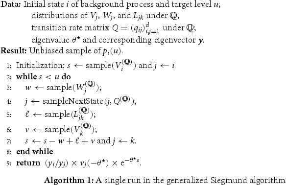
In this section, we point out how to efficiently estimate $p_i(u)$ by simulation, with emphasis on the regime that u is large. The main idea is to rely on importance sampling, using a generalized version of the celebrated Siegmund algorithm. More specifically, we propose to run independent simulations of the MAP under $\mathbb{Q}$, and subsequently average the values of $\gamma :=\frac{y_i}{y_{K_N}}{v}_{K_N}(-{\theta }^{\star }){\mathrm{e}}^{-{\theta }^{\star }{S}_N}$ that are sampled in each of the runs. By Theorem 3.1 this results in an unbiased estimator. The main objective of this section is to prove that this estimator has bounded relative error. Its efficiency gain (relative to direct simulation, that is) is demonstrated in Section 7 through a series of numerical experiments.

A pseudo-code corresponding to a single run of this generalized Siegmund algorithm is given by Algorithm 1. Here s records the current value of the embedded MAP and j the current background state. Also, the function ‘sample(X)’ generates and returns a sample of the random variable X, independent of everything what has been sampled before. Finally, the function ‘$\mathrm{sampleNextState}(j,Q^{(\mathbb{Q})})$’ returns a new state of the background chain sampled under $\mathbb{Q}$, when the current state is j.

The while loop in Algorithm 1 updates the value of the MAP at maxima between two successive background transition epochs. Lines 3 through 7 respectively correspond to sampling the decrease of the MAP before the next background transition, sampling the next background state, sampling the jump at the transition epoch and sampling the maximum between the current and next background transitions.

An important performance measure of algorithms estimating small probabilities is their relative error, defined by the standard deviation of the estimate divided by the estimated probability. Not only does $\gamma \equiv \gamma (u)$ yield an unbiased estimator of $p_i(u)$, the next theorem entails that the relative error is bounded in u. We refer to this property as bounded relative error (Asmussen & Glynn 2007, Ch. VI.1).

Theorem 6.1

A sample of $p_i(u)$ as returned by Algorithm 1 has bounded relative error.

Proof.

The proof is closely related to its counterpart for the random walk case (Asmussen & Glynn 2007, Ch. VI.2). Denote, in line with the notation that we have previously used, by $R(u)$ and $K_{N(u)}$ the overshoot and the background state, respectively, at the time that level u is crossed. Now consider the process $(R(u),K_{N(u)}{)}_{u⩾0}$, conditional on $K_0=i$. Above, we have computed the transform $r_{\mathrm{ij}}(\theta )$, by which we uniquely characterized the limiting distribution of $(R(u),K_{N(u)})$ as $u\to \mathrm{\infty }$; we let $(R,K)$ be distributed as the corresponding limiting random vector.

As a result of the above, the ruin probability (which equals the mean of $\gamma (u)$, as defined above) satisfies the following asymptotics, as $u\to \mathrm{\infty }$: $\begin{array}{rl}{\mathrm{e}}^{{\theta }^{\star }u}{\mathbb{E}}_{\mathbb{Q}}\gamma (u)& ={\mathrm{e}}^{{\theta }^{\star }u}{p}_i(u)={\mathbb{E}}_{\mathbb{Q}}(\frac{y_i}{y_{K_{N(u)}}}{v}_{K_{N(u)}}(-{\theta }^{\star }){\mathrm{e}}^{-{\theta }^{\star }(S_{N(u)}-u)})\\ & \to {\mathbb{E}}_{\mathbb{Q}}(\frac{y_i}{y_K}{v}_K(-{\theta }^{\star }){\mathrm{e}}^{-{\theta }^{\star }R})=\sum _{j=1}^d{r}_{\mathrm{ij}}({\theta }^{\star })\frac{y_i}{y_j}{v}_j(-{\theta }^{\star })=:C_1.\end{array}$ We have bounded relative error as the second moment of $\gamma (u)$ vanishes at essentially the same rate as the square of $p_i(u)$; to see this, observe that $\begin{array}{rl}{\mathrm{e}}^{2{\theta }^{\star }u}{\mathbb{E}}_{\mathbb{Q}}({\gamma }^2(u))& ={\mathrm{e}}^{2{\theta }^{\star }u}{\mathbb{E}}_{\mathbb{Q}}(\frac{y_i^2}{y_{K_{N(u)}}^2}{v}_{K_{N(u)}}^2(-{\theta }^{\star }){\mathrm{e}}^{-2{\theta }^{\star }{S}_{N(u)}})\\ & \to {\mathbb{E}}_{\mathbb{Q}}(\frac{y_i^2}{y_K^2}{v}_K^2(-{\theta }^{\star }){\mathrm{e}}^{-2{\theta }^{\star }R})=\sum _{j=1}^d{r}_{\mathrm{ij}}(2{\theta }^{\star }){(\frac{y_i}{y_j}{v}_j(-{\theta }^{\star }))}^2=:C_2,\end{array}$ where it is noted that $C_2>C_1^2$ due to Jensen's inequality. The variance of a single observation $\gamma (u)$ in our generalized Siegmund algorithm thus satisfies ${\mathrm{e}}^{2{\theta }^{\star }u}{\mathrm{Var}}_{\mathbb{Q}}(\frac{y_i}{y_{K_{N(u)}}}{v}_{K_{N(u)}}(-{\theta }^{\star }){\mathrm{e}}^{-{\theta }^{\star }{S}_{N(u)}})\to C_2-C_1^2.$ It now directly follows that for u large the relative error tends to (14) $c:=\frac{\sqrt{C_2-C_1^2}}{C_1}\in (0,\mathrm{\infty }).$(14) We observe that apparently the relative error loses its dependence on u as u grows, and that it is bounded by a constant.

7. Numerical experiments

In this section, we numerically study the asymptotic behavior of $p(u)$, measuring in particular the efficiency of the generalized Siegmund algorithm compared to direct estimation. We in addition include an experiment that studies the impact of the background process on the ruin probability.

To obtain a direct estimation of the ruin probability $p(u)$, one may simulate the model at hand say n times under the original measure $\mathbb{P}$, and then determine the fraction of runs in which the process exceeds level u. This leads to an unbiased estimator, with the relative error equaling $\frac{\sqrt{\frac{1}{n}p(u)(1-p(u))}}{p(u)}=\sqrt{\frac{1-p(u)}{\mathrm{np}(u)}}.$ In order to achieve a relative error of at most ϵ, one thus requires roughly $n\approx \frac{1-p(u)}{{ϵ}^{2}p(u)}$ runs. The particularly worrisome element in this quantity is the $p(u)$ in the denominator, being very small when u is large. Concretely, with $p(u)$ decaying roughly as ${\mathrm{e}}^{-{\theta }^{\star }u}$ and $1-p(u)\approx 1$, we conclude that n blows up like ${\mathrm{e}}^{{\theta }^{\star }u}$ as u grows.

The generalized Siegmund algorithm, in which the process is simulated under $\mathbb{Q}$, on the other hand has bounded relative error. With c given in (14(14) $c:=\frac{\sqrt{C_2-C_1^2}}{C_1}\in (0,\mathrm{\infty }).$(14) ), and again aiming for a relative error ϵ, this algorithm thus requires roughly $n\approx c/{ϵ}^2$ runs for large u. As a result, the generalized Siegmund algorithm gives an accurate estimation for any u, in that for large u the number of runs required becomes independent of u. This in particular means that this number of runs does not blow up as $p(u)\to 0$.

In the remainder of this section we discuss experiments in which we apply our generalized Siegmund algorithm. It should be noted that executing this algorithm requires being able to sample random variables $(V_k{)}_{k\in \{1,\dots ,d\}}$, while only their respective Laplace-Stieltjes transforms are known (see Proposition 2.1). To this end we first apply numerical inversion to obtain a discretization of the distribution function of each of the $V_k$. In our numerics we have used the intensively tested and frequently cited algorithm that was developed in Abate & Whitt (2006); in the experiments reported in this section, we use ${10}^3$ mass points. With this approximate distribution function at our disposal, we can use the inverse distribution function method to sample a random variable distributed according to $V_k$. Three remarks are in place here.

°	First observe that, for any k, the Laplace inversion has to be performed just once (say, in the pre-processing phase); once the approximate distribution function of $V_k$ has been computed, the generalized Siegmund algorithm can be repeatedly executed until an estimate of sufficient precision has been produced.
°	Secondly, the simulation of the embedded process under the original measure $\mathbb{P}$ has the same inherent issue that the $V_k$ must be sampled. In other words, the need to perform Laplace inversion is not specific for the generalized Siegmund algorithm.
°	The fact that we propose to use numerical Laplace inversion to run our generalized Siegmund algorithm, triggers the question why we do not simply numerically invert the transform of $p(u)$ (as was obtained in van Kreveld et al. (2022)). However, the latter method is typically inferior to the generalized Siegmund algorithm, in particular in the current context where the ruin probability $p(u)$ is small, as a consequence of the fact that the Laplace inversion becomes increasingly inaccurate further along the tail.

We now describe the specific MAP we use in our experiments. It consists of two background states, the first and second corresponding respectively to a standard Brownian motion $X_1(\cdot )$ with drift $-\frac{1}{3}$, and a compound Poisson process $X_2(\cdot )$ with drift $-1$ and jumps of $\mathrm{Exp}(1)$ size arriving at rate $\frac{2}{3}$. Note that we constructed this instance such that $\mathbb{E}{X}_1(1)=\mathbb{E}{X}_2(1)=-\frac{1}{3}$, allowing for better comparison between the impacts of both processes on the ruin probability. To make our model as elementary as possible, our setup does not contain jumps at transition epochs; we stress however that adding those does not lead to any conceptual complications.

Experiment 7.1

In the first experiment we vary the value of the exceedance level (or, in risk applications, the initial reserve) u, so as to provide empirical backing for the claims of Theorems 5.1 and 6.1. In addition, we obtain insight into the accuracy of the approximation (13(13) $p_i(u)\approx {\overline{p}}_i(u):={\alpha }_i{\mathrm{e}}^{-{\theta }^{\star }u}.$(13) ).

We consider the instance $q_1=q_2=1$, and we vary u (with steps of 10) from 10 to 80, see Table 1. Two approximations of the ruin probability are presented: the second column shows estimates of $p_1(u)$ that are generated by ${10}^4$ runs of Algorithm 1, and the third column presents the approximation ${\overline{p}}_1(u)={\alpha }_1{\mathrm{e}}^{-{\theta }^{\star }u}$ of (13(13) $p_i(u)\approx {\overline{p}}_i(u):={\alpha }_i{\mathrm{e}}^{-{\theta }^{\star }u}.$(13) ) (with ${\alpha }_1\approx 0.6390$ and ${\theta }^{\star }\approx 0.4066$). The approximations of both methods differ around $1\mathrm{\%}$, even for small values of u. This indicates, for our specific MAP, fast convergence of the expression in Theorem 5.1.

Table 1. Ruin probabilities as a function of u, and the relative error per run under $\mathbb{Q}$ and $\mathbb{P}$.

u	$p_1(u)$ estimated by Algorithm 1	${\alpha }_1{\mathrm{e}}^{-{\theta }^{\star }u}$	Relative error per run under $\mathbb{Q}$	Relative error per run under $\mathbb{P}$
10	$1.084\cdot {10}^{-2}$	$1.09537\cdot {10}^{-2}$	0.623	9.55
20	$1.862\cdot {10}^{-4}$	$1.87784\cdot {10}^{-4}$	0.630	73.3
30	$3.224\cdot {10}^{-6}$	$3.21924\cdot {10}^{-6}$	0.626	$5.57\cdot {10}^2$
40	$5.519\cdot {10}^{-8}$	$5.51886\cdot {10}^{-8}$	0.622	$4.26\cdot {10}^3$
50	$9.460\cdot {10}^{-10}$	$9.46117\cdot {10}^{-10}$	0.623	$3.25\cdot {10}^4$
60	$1.620\cdot {10}^{-11}$	$1.62196\cdot {10}^{-11}$	0.629	$2.48\cdot {10}^5$
70	$2.789\cdot {10}^{-13}$	$2.78058\cdot {10}^{-13}$	0.621	$1.89\cdot {10}^6$
80	$4.798\cdot {10}^{-15}$	$4.76685\cdot {10}^{-15}$	0.619	$1.44\cdot {10}^7$

In addition, Table 1 shows the average relative error of a single run under $\mathbb{Q}$ (Algorithm 1), based on the sample (fourth column). This is compared to the same error when one would estimate the ruin probability directly under $\mathbb{P}$ (fifth column). Where the relative error of Algorithm 1 is fairly constant, the same error under direct estimation shows exponential increase in u, as anticipated. If, say, one is interested in an estimate for $p_1(u)$ with relative error at most $5\mathrm{\%}$, the instances u = 10, 40, 80 respectively require approximately $4\cdot {10}^4$, $7\cdot {10}^9$, and $8\cdot {10}^{16}$ runs. The number of runs required under $\mathbb{Q}$, on the other hand, is around 250 for any value of u.

Experiment 7.2

In the second experiment the background chain transition rates $q_1$ and $q_2$ are varied, and with them the proportion of time spent in each of the two background states. For each combination of these parameter values we run Algorithm 1 with u = 40 a total of ${10}^4$ times. The output consists of the estimated ruin probability and the relative error per run based on the sample. The results are shown in Table 2.

Table 2. Ruin probabilities as a function of the fraction of time spent in each of the two background states.

$q_1$	$q_2$	Fraction of time in state 1	$p_1(40)$	Relative error per run
${10}^4$	1	$1/10001$	$1.078\cdot {10}^{-6}$	0.520
${10}^3$	1	$1/1001$	$1.072\cdot {10}^{-6}$	0.519
${10}^2$	1	$1/101$	$1.026\cdot {10}^{-6}$	0.527
10	1	$1/11$	$7.043\cdot {10}^{-7}$	0.536
5	1	$1/6$	$4.873\cdot {10}^{-7}$	0.543
2	1	$1/3$	$1.833\cdot {10}^{-7}$	0.577
1	1	$1/2$	$5.519\cdot {10}^{-8}$	0.622
1	2	$2/3$	$1.075\cdot {10}^{-8}$	0.594
1	5	$5/6$	$8.559\cdot {10}^{-10}$	0.584
1	10	$10/11$	$1.374\cdot {10}^{-10}$	0.575
1	${10}^2$	$100/101$	$5.005\cdot {10}^{-12}$	0.465
1	${10}^3$	$1000/1001$	$2.821\cdot {10}^{-12}$	0.408
1	${10}^4$	$10000/10001$	$2.629\cdot {10}^{-12}$	0.408

As we can see, the ruin probability heavily depends on the transition rates of the background chain. The larger the proportion of time spent in the compound Poisson state (state 2), the larger the ruin probability, and the larger the proportion of time spent in the Brownian state (state 1), the smaller the ruin probability. It is also reassuring to see that, for this MAP, the (bounded) relative error per run is rather low. With ${10}^4$ runs this results in a relative error in the order of $5\cdot {10}^{-3}$.

When $q_1>>q_2$, one expects that the net cumulative claim process effectively coincides with a compound Poisson process, which has a ruin probability that asymptotically decays as $\frac{2}{3}{\mathrm{e}}^{-\frac{u}{3}}$. Substituting u = 40 gives $1.0797\cdot {10}^{-6}$, close to the values of $p_1(40)$ in the top rows. Conversely, when $q_1<<q_2$, the net cumulative claim process should be close to a Brownian motion, which has a ruin probability ${\mathrm{e}}^{-\frac{2}{3}u}$. Substituting u = 40 gives $2.6231\cdot {10}^{-12}$, in line with the values of $p_1(40)$ in the bottom rows.

8. Discussion and concluding remarks

In this paper we have considered a ruin model driven by a light-tailed spectrally-positive Markov additive process. We first identified the exact asymptotics of the ruin probability, and then devised an efficient simulation algorithm. Since previous literature restricts to MAPs with specific underlying Lévy processes, our results narrow the gap in the understanding of these asymptotics for arbitrary MAPs. Nevertheless, various directions for further research are possible, of which we list a few.

When the net cumulative claim process is a spectrally-negative MAP (i.e. having jumps in the downward direction only), the all-time maximum has a phase-type distribution (van Kreveld et al. 2022). This means that in that case the exact asymptotics of the ruin probability can be dealt with relatively easily. Considerably more challenging, however, is the case of a MAP with jumps in both directions; this would extend the result for the Lévy case that was established in Bertoin & Doney (1994). A possible first step in this direction could be to assume that the jumps in one of the directions are of phase-type (cf. Jacobsen 2005 for instance).

A second interesting extension would concern the inclusion of heavy-tailed jump size distributions, applying to jumps of the Lévy processes and/or jumps at transition epochs. Such distributions deny the existence of a positive solution ${\theta }^{\star }$ to the Lundberg equation, thus invalidating our change-of-measure approach. Instead, we suggest to build upon the results of Foss et al. (2007), in which the ‘principle of a single big jump’ is exploited.

In our paper we used an embedded process to simplify the analysis while maintaining all information on the ruin probability over level u. For this embedded process, we in particular identified the transform $s_{\mathrm{ij}}(\alpha ,\theta )$ of the overshoot over level u. However, it is clear that the overshoot over level u of the embedded process can be substantially different from its counterpart for the original MAP. This leaves open the problem of characterizing the distribution of the overshoot for our MAP. Extensions in this direction would be valuable additions to the literature on first passage times.

Finally, it may be interesting to explore which results can be obtained if one drops the assumption that the background chain is irreducible, but still assumes that the asymptotic drift in the recurrent classes is negative. In this setting we think it is wise to condition on the joint distribution of the recurrent class that is reached and the value of the MAP at the time this class is reached. We conjecture that, out of the reachable recurrent classes from the initial state, only the class with the lowest exponential decay rate (i.e. with the heaviest tail) impacts the ruin probability in the $u\to \mathrm{\infty }$ limit.

Acknowledgments

The authors thank Onno Boxma (Eindhoven University of Technology), Masakiyo Miyazawa (Tokyo University of Science), and Peter Spreij (University of Amsterdam) for useful remarks.

Disclosure statement

No potential conflict of interest was reported by the author(s).

Additional information

Funding

This research is partly funded by the Nederlandse Organisatie voor Wetenschappelijk Onderzoek (NWO) Gravitation Project Networks [grant number 024.002.003].

References

- Abate J. & Whitt W. (2006). A unified framework for numerically inverting Laplace transforms. INFORMS Journal on Computing 18(4), 408–421.
- Asmussen S. (2003). Applied probability and queues, 2nd ed. New York: Springer.
- Asmussen S. & Albrecher H. (2010). Ruin probabilities. Singapore: World Scientific.
- Asmussen S. & Glynn P. (2007). Stochastic simulation: algorithms and analysis. New York: Springer.
- Bertoin J. & Doney R. (1994). Cramér's estimate for Lévy processes. Statistics & Probability Letters 21(5), 363–365.
- Çinlar E. (1972). Markov additive processes. I. Zeitschrift für Wahrscheinlichkeitstheorie und Verwandte Gebiete 24(2), 85–93.
- D'Auria B., Ivanovs J., Kella O. & Mandjes M. (2010). First passage of a Markov additive process and generalized Jordan chains. Journal of Applied Probability 47(4), 1048–1057.
- Debicki K. & Mandjes M. (2015). Queues and Lévy fluctuation theory. New York: Springer.
- Dieker A. B. & Mandjes M. (2011). Extremes of Markov-additive processes with one-sided jumps, with queueing applications. Methodology and Computing in Applied Probability 13(2), 221–267.
- Foss S., Konstantopoulos T. & Zachary S. (2007). Discrete and continuous time modulated random walks with heavy-tailed increments. Journal of Theoretical Probability 20(3), 581–612.
- Ivanovs J. (2011). One-sided Markov additive processes and related exit problems [Ph.D. thesis]. University of Amsterdam. Available at: https://pure.uva.nl/ws/files/1408093/94456_0_Thesis.pdf
- Ivanovs J., Boxma O. & Mandjes M. (2010). Singularities of the matrix exponent of a Markov additive process with one-sided jumps. Stochastic Processes and Their Applications 120(9), 1776–1794.
- Jacobsen M. (2005). The time to ruin for a class of Markov additive risk process with two-sided jumps. Advances in Applied Probability 37(4), 963–992.
- Jasiulewicz H. (2001). Probability of ruin with variable premium rate in a Markovian environment. Insurance: Mathematics and Economics 29(2), 291–296.
- Kyprianou A. (2006). Introductory lectures on fluctuations of Lévy processes with applications. New York: Springer.
- Miyazawa M. (2002). A Markov renewal approach to the asymptotic decay of the tail probabilities in risk and queuing processes. Probability in the Engineering and Informational Sciences 16(2), 139–150.
- Miyazawa M. (2004). Hitting probabilities in a Markov additive process with linear movements and upward jumps: applications to risk and queueing processes. The Annals of Applied Probability 14(2), 1029–1054.
- Neveu J. (1961). Une généralisation des processus à accroissements positifs indépendents. Abhandlungen aus dem Mathematischen Seminar der Universität Hamburg 25(1-2), 36–61.
- Siegl T. & Tichy R. F. (1999). A process with stochastic claim frequency and a linear dividend barrier. Insurance: Mathematics and Economics 24(1-2), 51–65.
- van Kreveld L., Mandjes M. & Dorsman J. (2022). Extreme value analysis for a Markov additive process driven by a nonirreducible background chain. Stochastic Systems 12(3), 293–317.
- Yin G., Liu Y. J. & Yang H. (2006). Bounds of ruin probability for regime-switching models using time scale separation. Scandinavian Actuarial Journal 2006(2), 111–127.
- Zhu J. & Yang H. (2009). On differentiability of ruin functions under Markov-modulated models. Stochastic Processes and Their Applications 119(5), 1673–1695.