Intracerebral Hemorrhage Detection in Computed Tomography Scans Through Cost-Sensitive Machine Learning

ABSTRACT

Intracerebral hemorrhage is the most severe form of stroke, with a greater than 75% likelihood of death or severe disability, and half of its mortality occurs in the first 24 hours. The grave nature of intracerebral hemorrhage and the high cost of false negatives in its diagnosis are representative of many medical tasks. Cost-sensitive machine learning has shown promise in various studies as a method of minimizing unwanted results. In this study, 6 machine learning models were trained on 160 computed tomography brain scans both with and without utility matrices based on penalization, an implementation of cost-sensitive learning. The highest-performing model was the support vector machine, which obtained an accuracy of 97.5%, sensitivity of 95% and specificity of 100% without penalization, and an accuracy of 92.5%, sensitivity of 100% and specificity of 85% with penalization, on a test dataset of 40 scans. In both cases, the model outperforms a range of previous work using other techniques despite the small size of and high heterogeneity in the dataset. Utility matrices demonstrate strong potential for sensitive yet accurate artificial intelligence techniques in medical contexts and workflows where a reduction of false negatives is crucial.

Introduction

Intracerebral hemorrhage (ICH) is a neurological condition occurring due to the rupture of blood vessels in the brain parenchyma (Badjatia and Rosand 2005). It is the most severe form of stroke, with the chance of death or severe disability exceeding 75% and only 20% of survivors remaining capable of living independently after 1 month (Nawabi et al. 2021; Xinghua et al. 2021). It has an incidence of 24.6 per 100,000 person-years and accounts for 10–15% of all strokes (Ziai and Ricardo Carhuapoma 2018). An early diagnosis of ICH is crucial as half of the mortality occurs in the first 24 hours (Arbabshirani et al. 2018). Computed tomography (CT) scans are currently the preferred noninvasive approach for ICH detection (Hai et al. 2019). The diagnosis time for ICH remains very long—reaching 512 minutes in one study—which couples with a high misdiagnosis rate—13.6% according to one estimate—to make it a prime candidate for workflow improvement through machine learning (Arbabshirani et al. 2018; Hai et al. 2019).

The conditions and characteristics that are specific to the medical field must be taken into consideration during the application of machine learning techniques to problems such as ICH diagnosis. A primary concern is that false negatives are usually much more costly than false positives (Claude and Webb 2011). The frequent under-representation of the minority class coupled with the increased emphasis on its correct prediction makes this a challenging problem for artificial intelligence (Thai-Nghe, Gantner, and Schmidt-Thieme 2010).

Taking the disproportionate costs of false negatives into account—more broadly called cost-sensitive learning—has resulted in positive outcomes in other medical tasks (Charoenphakdee et al. 2021; Freitas, Costa-Pereira, and Brazdil 2007; Fuqua and Razzaghi 2020; Kukar et al. 1999; Septiandri et al. 2020; Siddiqui et al. 2020; Tianyang et al. 2020)

However, there is very little literature on the application of such techniques in hemorrhage diagnosis. Hence, the aim of this research was to test the results of the implementation of cost-sensitive learning—specifically a utility matrix-based approach—on ICH classification.

Materials and Methods

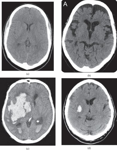
The data used for the study were obtained under a CC0: Public Domain license (Kitamura 2017). The dataset consisted of 200 anonymized, publicly-available images of non-contrast computed tomography (CT) scans (brain window), 100 of which contained instances of intraparenchymal hemorrhage with or without intraventricular extension, and 100 of which did not. A sample of 4 images from the data is shown in Figure 1. Figure 1a,b show scans without intracerebral hemorrhage, at the level of the lateral ventricles and third ventricle, respectively. Figure 1c displays a large intracerebral hemorrhage with intraventricular extension. Figure 1d contains a small intracerebral hemorrhage without intraventricular extension.

Figure 1. Sample dataset images.

A trained radiologist confirmed the veracity of these images, and was unable to find any mislabeled images. Thus none of the images was discarded. To obtain the most accurate representation of model performance in real-life clinical scenarios, the images were not augmented in any way. Two datasets were subsequently created: a training dataset with 160 images and a testing dataset with 40 images. Both had equal numbers of hemorrhagic and non-hemorrhagic CT scans. It should be noted that the dataset consisted of images taken from searches on the World Wide Web, hence introducing a high level of heterogeneity due to variations in source machines, patient conditions, scan time, radiation dose, etc. This problem is compounded by the small dataset size, thus the results obtained here are likely to only be conservative estimates of the real potential of the techniques employed (Lacroix and Critchlow 2003; Lim et al. 2019).

6 machine learning models were chosen for the study. The specific parameter configurations for these models are provided in Table 1, and are important for reproducibility. A random seed of 0 was used in each case. The models were trained using Wolfram Mathematica Desktop Version 12.3.0, making use of the Classify[] function (Wolfram Research 2021).

Table 1. Parameter specifications.

Name	Parameters
Random Forest	FeatureFraction = $\frac{1}{4\sqrt{10}}$, LeafSize = 5, TreeNumber = 50, DistributionSmoothing = 0.5
Decision Tree	DistributionSmoothing = 1, FeatureFraction = 1
Gradient Boosted Trees	BoostingMethod = Gradient, MaxTrainingRounds = 50, LeavesNumber = 13, LearningRate = 0.1, MaxDepth = 6, LeafSize = 15, L1Regularization = 0, L2Regularization = 0
Nearest Neighbors	NeighborsNumber = 5, DistributionSmoothing = 0.5, NearestMethod = Scan
Support Vector Machine	KernelType = RadialBasisFunction, GammaScalingParameter = 0.00113124, PolynomialDegree = 3, SoftMarginParameter = 1, BiasParameter = 1, MulticlassStrategy = OneVersusOne
Logistic Regression	L1Regularization = 0, L2Regularization = 100, OptimizationMethod = LBFGS

Decision Tree

A decision tree is a machine learning model that consists of nodes and branches, and is built using a combination of splitting, stopping and pruning (Song and Ying 2015). Combining all of these techniques, while not guaranteed to result in the theoretically-optimal decision tree – as that would require an exceedingly long time – still results in a highly useful model (Swain and Hauska 1977).

Nodes and Branches

The root node is the first node, and it represents a decision that divides the entire data into two or more subsets. Internal nodes represent more choices that can be used to further split subsets. Eventually, they end in leaf nodes, representing the final result of a series of choices. Any node emanating from another node can be referred to as its child node. Branches are representations of the outcomes of decisions made by nodes and connect them to their child nodes (Song and Ying 2015).

Splitting

Both discrete or continuous variables can be used by decision trees to set criteria for different nodes, either internal or root, that are used to split the data into multiple internal or leaf nodes. Decision trees choose between different splitting possibilities using certain measures of the child nodes, such as entropy, Gini index, and information gain, to optimize the splitting choices (Song and Ying 2015).

Stopping

If allowed to split indefinitely, a decision tree model could achieve 100% accuracy simply by splitting over and over until each leaf node only had one data sample. However, such a model would be vastly overfitted and would not generalize well to test data. Thus there needs to be a limit (often in the form of maximum depth allowed or minimum size of leaf nodes) (Song and Ying 2015).

Pruning

There are two types of pruning. Pre-pruning uses multiple-comparison tests to stop the creation of branches that are not statistically significant, whereas post-pruning removes branches from a fully-generated decision tree in a way that increases accuracy on the validation set, which is a special subset of the training data not shown to the model while training (Song and Ying 2015).

Random Forest

A random forest, as the name suggests, is a collection of randomized decision trees that is suitable for situations where a simple decision tree could not capture the complexity of the task at hand (Breiman 2001). The random forest model performs a “bootstrap” by choosing n times from n decision trees with replacement (Biau and Scornet 2016). The averaging of these predictions is called bagging (short for bootstrap-aggregating) and is a simple way to improve the performance of weak models, which many decision trees are when the task is complex (Breiman 1996).

Gradient Boosted Trees

Gradient tree boosting constructs an additive model, using decision trees as weak learners to aggregate, similar to the concept of random forests, but it does so sequentially; gradient descent is then used to minimize a given loss function and optimize the construction of the model as more trees are added (Friedman 2001; Jerry et al. 2009).

Nearest Neighbors

The nearest neighbors model is based on the concept that the closest patterns of the data sample in question offer useful information about its classification. Thus the model works by assigning each data point the label of its k closest neighbors, where k is specified manually (Kramer 2013).

Support Vector Machine

Support vector machines, linear and nonlinear, are a family of modular machine learning algorithms for binary classification problems by using principles from convex optimization and statistical learning theory (Mammone, Turchi, and Cristianini 2009).

Separating Hyperplane

For n-dimensional data, a hyperplane (straight line in a higher-dimensional space) of n-1 dimensions is used to separate the data into two different groups such that the distance from the clusters is maximized and the hyperplane is “in the middle,” so to speak. This hyperplane also dictates which labels will be assigned to the samples from the test set (Noble 2006).

Soft Margin

Most datasets, of course, do not have clean boundaries separating different clusters of samples. There will also be outliers, and an optimal model would allow for a certain number of outliers to avoid overfitting while also limiting misclassifications. The soft margin roughly controls the number of examples allowed on the wrong side of the hyperplane as well as their distance from the hyperplane (Noble 2006).

Kernel Function

A kernel function refers to one or more mathematical operations that project low-dimensional data to a higher-dimensional space called a feature space, with the goal being the easier separation of the example data (Suthaharan 2016).

Logistic Regression

Logistic regression is a mathematical model that describes the relationship of a number of features ($X_1,X_2,\dots ,X_k$) to a dichotomous result. It makes use of the logistic function to assign probabilities to samples of belonging to either class, and the sample is then classified to the class where it has the higher probability of belonging (Kleinbaum and Klein 2010).

Utility Matrices

For the second part of the study, the concept of utility functions was used. A utility function is a mathematical function through which preferences for various outcomes can be quantified (Russell and Norvig 2002). In the case of a utility matrix for classification problems, $U_{ij}$ provides the utility where $i$ is the ground truth and $j$ is the model prediction reference (Wolfram Research 2014). It is also referred to as a cost matrix (Elkan 2001).

The utility matrix created for this study is shown in Table 2. The sole difference from the default utility matrix is that false negatives (Row 1, Column 2) now have a utility of -$x$ instead of 0. Subsequent experimentation with different values of $x$ was done and the results were recorded.

Table 2. Utility matrix used for this study.

	Hemorrhage	No Hemorrhage
Hemorrhage	$1$	-$x$
No Hemorrhage	$0$	$1$

Essentially, the models trained using this matrix will have an aversion to false negatives, thus decreasing the number of false negatives at the expense of potentially increasing the number of false positives. The strength of this aversion and subsequent change is quantified by $x$. A certain amount of trial and error is needed since, for most medical problems, the cost is not certain and needs to be estimated (Wang, Kou, and Peng 2021). The cost is context-specific; depending on the workflow where the algorithm is being implemented, the goals for sensitivity and specificity will vary and the cost must be determined accordingly.

In Round 2, the models were re-trained with the same parameters as the previous set, with the only difference being that the value for the “UtilityFunction” parameter was set to the utility matrix provided in Table 2.

Results

The final results for all of the models trained are given in Table 3. The probability histograms for the 3 most accurate models are given in Figure 2. These histograms show the actual-class probability of the 40 test samples. Table 4 lists the results for each of the models after setting their utility function to the matrix given in Table 2, for three values of $-x$. Finally, Figure 3 shows, for the top three models, how their sensitivities and specificities change as the penalty is increased, with 0 being the default penalty that corresponds to Table 3.

Figure 2. Probability histograms.

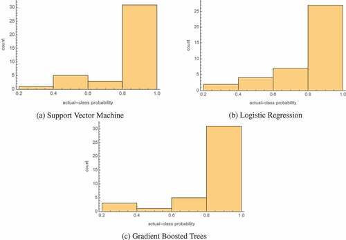
Figure 3. Trends for sensitivities and specificities by penalty.

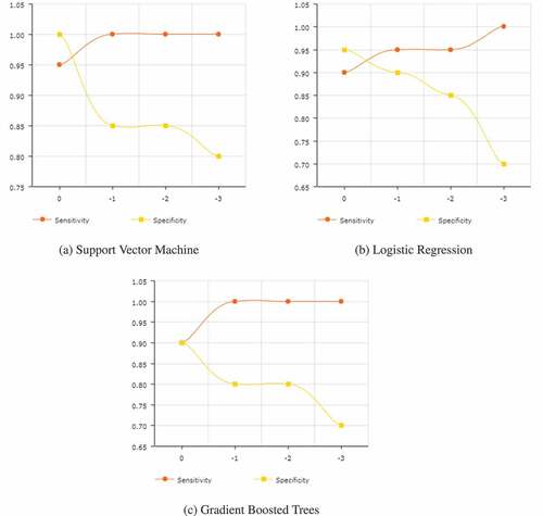
Table 3. Round 1 results.

	Accuracy	Sensitivity	Specificity
Decision Tree	0.600	0.800	0.400
Random Forest	0.700	0.750	0.650
Gradient Boosted Trees	0.900	0.900	0.900
Nearest Neighbors	0.825	0.700	0.950
Support Vector Machine	0.975	0.950	1.00
Logistic Regression	0.925	0.900	0.950

Table 4. Round 2 results.

	Penalty of −1			Penalty of −2			Penalty of −3
	Acc	Sens	Spec	Acc	Sens	Spec	Acc	Sens	Spec
Decision Tree	0.500	1.00	0	0.500	1.00	0	0.500	1.00	0
Random Forest	0.650	0.900	0.400	0.650	0.900	0.400	0.700	1.00	0.400
Gradient Boosted Trees	0.900	1.00	0.800	0.900	1.00	0.800	0.850	1.00	0.700
Nearest Neighbors	0.800	0.900	0.700	0.800	0.900	0.700	0.625	0.950	0.300
Support Vector Machine	0.925	1.00	0.850	0.925	1.00	0.850	0.900	1.00	0.800
Logistic Regression	0.925	0.950	0.900	0.900	0.950	0.850	0.850	1.00	0.700

According to the data in Table 3, the support vector machine model is the most accurate as well as the most sensitive and specific. Logistic regression and gradient boosted trees score second and third respectively in overall accuracy, though the nearest neighbors model has a higher specificity than gradient boosted trees, coming in second and tied with logistic regression.

Interestingly, while Table 3 shows that the support vector machine is more accurate overall, logistic regression actually appears to be more certain in its predictions, as demonstrated by the difference in the number of samples in the 0.4–0.6 bin. Overall, though, all three of the best-performing models seem highly certain in the correct predictions that they are making, as the vast majority of samples fall in the 0.8–1.0 bin.

In Table 4, for a penalty of −1, three models give a 100% sensitivity, although for the decision tree that comes at the cost of having a 0% specificity. The support vector machine performs the best, matching the 100% sensitivity of gradient boosted trees. Its specificity of 85% is less than that achieved by logistic regression, though its sensitivity is greater.

The results for a −2 penalty are almost exactly the same, with the only difference being a slightly reduced accuracy for logistic regression.

When the penalty is increased to −3, model performances decrease along the board, except for random forest, which performs better). While the sensitivities for almost all the models are now 100%, they come at the expense of drastically reduced specificities.

Further values of $-x$ were not tested as most model performances had started rapidly deteriorating at a −3 penalty. The random forest, however, might perform better at more negative penalties, based on the observed trends.

As expected, Figure 3 shows that greater penalties yield reductions in specificity and growth in sensitivity. Though in cases like Figures 3a,c, where the sensitivity maxes out early, additional penalties only decrease the specificity. While tweaking the penalties, some changes, such as the one 0.85 to 0.70 in the specificity in Figure 3b, can be quite drastic, making it all the more important to conduct detailed experimentation while determining the penalty.

Discussion

The Round 1 results compare favorably to prior studies conducted for ICH identification, especially taking into the account the small training set and heterogeneity in the training data. For instance, work done by Majumdar et al. (Majumdar et al. 2018) shows a sensitivity of 81% and specificity of 98%. In one study, the model accuracy of 82%, recall of 89% and precision of 81% remarkably still resulted in a better recall than 2 of the 3 senior radiologists used for benchmarking (Grewal et al. 2018). More recent research by Dawud et al. (Dawud, Yurtkan, and Oztoprak 2019) resulted in the development of three models, with accuracies of 90%, 92% and 93%. Jnawali et al. (2018) performed a study with dataset heterogeneity comparable to ours, although with a considerably larger dataset size of 1.5 million images, and achieved an AUC score of 0.87. A study using 37,000 training samples, also with pronounced heterogeneity in the dataset, obtained an accuracy of 84%, a sensitivity of 70%, and a specificity of 87% (Arbabshirani et al. 2018). A retrospectively-collected dataset of 3605 scans was used to evaluate a commercial artificial intelligence decision support system (AIDSS) and showed a sensitivity of 92.3% and a specificity of 97.7% (Voter et al. 2021). There were also two studies that achieved better accuracies of 99% and one study with an AUC of 0.991 (Bobby and Annapoorani 2021; Tog˘açar et al. 2019; Weicheng et al. 2019).

Recently, a new type of neural network was developed; 90 versions were trained and tested on ICH detection ability, with the best model attaining an accuracy of 83.3% (J. Y. Lee et al. 2020). The important similarity between the work of Lee et al. is the comparable dataset size of 250 images, split into 166 scans for training and 84 for testing. Thus, given the data available, the model presented in this paper surpasses prior performance. In another paper, a nature-inspired gray wolf optimizer (GWO) algorithm called GWOTLT was trained and tested, using 10-fold cross-validation, on the same dataset as the one used in this study. The baseline VGG-16 had a precision and recall of 88.6% and 86.0% respectively, while the improved GWOTLT achieved a precision of 90.9% and a recall of 93.0%, thus demonstrating that the performance here compares favorably to research utilizing the same data (Vrbančič, Zorman, and Podgorelec 2019).

As for cost-sensitive machine learning, only one example could be found for the application of such a technique on intracerebral hemorrhage in prior literature, where the authors ended up achieving an overall sensitivity of 96% and specificity of 95% on a training dataset of 904 cases; the cost in this case was introduced through a modified loss function instead of a utility matrix (used in this study) (H. Lee et al. 2019). A smaller training dataset of 160 images combined with greater heterogeneity likely reduced model performances in this study compared to Lee et al.’s work (Lacroix and Critchlow 2003; Lee et al. 2019; Lim et al. 2019).

The accuracy of the cost-sensitive support vector machine exceeds a number of prior studies’ performances. Comparing the accuracy against the array of research mentioned previously, it manages an accuracy greater than the models constructed by Dawud et al., Grewal et al., Arbabshirani et al. and Jnawali et al., while still maintaining a 100% sensitivity (Arbabshirani et al. 2018; Dawud, Yurtkan, and Oztoprak 2019; Grewal et al. 2018; Jnawali et al. 2018). As Rane and Warhade pointed out in their literature review, a cost-sensitive algorithm shows great potential as a strategy for more effective diagnosis, and the results confirm this, with the cost-sensitive models demonstrated here outperforming a number of other techniques (Rane and Warhade 2021).

Applications

Considering the details of utility matrix application and the results it produces, such a type of optimization is suited for a workflow where the artificial intelligence is not working in isolation. Since penalization for false negatives can end up reducing specificities, a further test might become necessary, whether it is a separate algorithm, human clinician(s), or something else. Cost-sensitive learning is ideal in situations where misdiagnosing a positive case could have serious negative impacts, but at the same time the misdiagnosis of a negative case would not cause much inconvenience.

Limitations and Future Research

Two limitations of this study were, as mentioned, the small sample size and high heterogeneity within the dataset. Due to the nature of the dataset, distinctions based on sex, ethnicity or age weren’t possible Future research that applies cost-sensitive techniques to larger, more standardized datasets, as well as utilizing datasets with details about sex, age, ethnicity, etc., could offer greater insights into the advantages and drawbacks of cost-sensitive AI algorithms, however this study is quite beneficial as a starting point for the novel application of utility matrices in pertinent medical scenarios.

Conclusion

Clearly, utility matrices have potential as a tool for minimizing unwanted false negatives while still providing accurate overall results. There is a trade-off between sensitivity and specificity, and a suitable value must be chosen after multiple trial and error estimates, but once the ideal penalty has been determined, a cost-sensitive model achieves the given goal better than a more general technique. More work should be done on a variety of use cases, but the initial results are promising.

Ethical Declarations

This research study was conducted retrospectively using human subject data made available in open access. Ethical approval was not required as confirmed by the institutional review board (IRB) of the Sri Aurobindo Institute of Medical Sciences in Indore, India.

Disclosure Statement

No potential conflict of interest was reported by the author(s).

Data Availability Statement

The dataset employed was provided under a CC0: Public Domain license by Kitamura (2017). The code for the study can be accessed at https://github.com/rushankgoyal/cost-sensitive-hemorrhage.

Additional information

Funding

No funding was received for conducting this study. The author has no relevant financial or non-financial interests to disclose.

References

- Arbabshirani, M. R., B. K. Fornwalt, G. J. Mongelluzzo, J. D. Suever, B. D. Geise, A. A. Patel, and G. J. Moore. 2018. Advanced machine learning in action: Identification of intracranial hemorrhage on computed tomography scans of the head with clinical workflow integration. Npj Digital Medicine 1 (9):1–3343. ISSN: 2398-6352. doi:10.1038/s41746-017-0015-z.
- Badjatia, N., and J. Rosand. 2005, November. Intracerebral hemorrhage. The Neurologist 11 (6):311–24. ISSN: 1074-7931. doi: https://doi.org/10.1097/01.nrl.0000178757.68551.26.
- Biau, G., and E. Scornet. 2016, June. A random forest guided tour. Test 25 (2):197–227. ISSN: 1863-8260. doi: 10.1007/s11749-016-0481-7.
- Bobby, J. S., and C. L. Annapoorani. 2021. Analysis of intracranial hemorrhage in Ct brain images using machine learning and deep learning algorithm. Annals of RSCB 25 (6):13742–52. https://www.annalsofrscb.ro/index.php/journal/article/view/8186.
- Breiman, L. 1996, August. Bagging predictors. Machine Learning 24 (2):123–40. ISSN: 1573-0565. doi: 10.1007/BF00058655.
- Breiman, L. 2001, October. Random forests. Machine Learning 45 (1):5–32. ISSN: 1573-0565. doi: 10.1023/A:1010933404324.
- Charoenphakdee, N., Z. Cui, Y. Zhang, and M. Sugiyama. 2021, July. “Classification with rejection based on cost-sensitive classification.” In International Conference on Machine Learning, 1507–17. PMLR. http://proceedings.mlr.press/v139/charoenphakdee21a.html.
- Claude, S., and G. I. Webb. 2011, March. Encyclopedia of machine learning. New York: Springer. https://www.amazon.com/Encyclopedia-Machine-Learning-Claude-Sammut/dp/0387307680.
- Dawud, A. M., K. Yurtkan, and H. Oztoprak. 2019, June. Application of deep learning in neuroradiology: Brain haemorrhage classification using transfer learning. Computational Intelligence and Neuroscience 2019:4629859. ISSN: 1687-5265. doi:10.1155/2019/4629859.
- Elkan, C. 2001, August. The foundations of cost-sensitive learning. In IJCAI’01: Proceedings of the 17th international joint conference on Artificial intelligence, vol. 2, 973–78. San Francisco, CA, USA: Morgan Kaufmann Publishers Inc. ISBN: 978-155860812. 10.5555/1642194.1642224
- Freitas, A., A. Costa-Pereira, and P. Brazdil. 2007, September. Cost-sensitive decision trees applied to medical data. In Data warehousing and knowledge discovery, 303–12. Berlin, Germany: Springer. ISBN: 978-3-540-74552-5. 10.1007/978-3-540-74553-2_28
- Friedman, J. H. 2001, October. Greedy function approximation: A gradient boosting machine. Annals of Statistics 29 (5):1189–232. ISSN: 0090-5364. doi: https://doi.org/10.1214/aos/1013203451.
- Fuqua, D., and T. Razzaghi. 2020, July. A cost-sensitive convolution neural network learning for control chart pattern recognition. Expert Systems with Applications 150:113275. ISSN: 0957-4174. doi:10.1016/j.eswa.2020.113275.
- Grewal, M., M. Mayank Srivastava, P. Kumar, and S. Varadarajan. 2018, April. “Radnet: Radiologist level accuracy using deep learning for hemorrhage detection in CT scans.” In 2018 IEEE 15th International Symposium on Biomedical Imaging (ISBI 2018), 281–84. IEEE. doi:10.1109/ISBI.2018.8363574.
- Hai, Y., F. Gao, Y. Yin, D. Guo, P. Zhao, Y. Lu, X. Wang, J. Bai, K. Cao, and Q. Song. 2019, November. Precise diagnosis of intracranial hemorrhage and subtypes using a three-dimensional joint convolutional and recurrent neural network. European Radiology 29(11): 6191–201. ISSN: 1432-1084. 10.1007/s00330-019-06163-2
- Jerry, Y., J.-H. Chow, J. Chen, and Z. Zheng. 2009, November. Stochastic gradient boosted distributed decision trees. In CIKM ‘09: Proceedings of the 18th ACM conference on Information and knowledge management, 2061–64. New York: Association for Computing Machinery. 978-1-60558512-3. 10.1145/1645953.1646301
- Jnawali, K., M. R. Arbabshirani, N. Rao, and A. A. Patel. 2018, February. Deep 3D convolution neural network for CT brain hemorrhage classification. In Medical imaging 2018: Computer-aided diagnosis, 10575:105751C. International Society for Optics/Photonics. 10.1117/12.2293725
- Kitamura, Felipe. 2017, August. Head CT - hemorrhage [Online]. Accessed July 22, 2021. https://www.kaggle.com/ felipekitamura/head-ct-hemorrhage
- Kleinbaum, D. G., and M. Klein. 2010, March. Introduction to logistic regression. In Logistic regression, 1–39. New York, NY, USANew York, NY: Springer. ISBN: 978-1-4419-1741-6. 10.1007/978-1-4419-1742-3_1
- Kramer, O. 2013. K-Nearest Neighbors. Dimensionality reduction with unsupervised nearest neighbors, 13–23. Berlin, Germany: Springer. ISBN: 978-3-642-38651-0. 10.1007/978-3-642-38652-7_2
- Kukar, M., I. Kononenko, C. Grošelj, K. Kralj, and J. Fettich. 1999. Analysing and improving the diagnosis of ischaemic heart disease with machine learning. Artificial Intelligence in Medicine 16 (11):25–50 ISSN: 0933-3657. doi:10.1016/S0933-3657(98)00063-3.
- Lacroix, Z., and T. Critchlow. 2003, January. Compared evaluation of scientific data management systems. In Bioinformatics, 371–91. ISBN: 978-1-55860-829-0. Morgan Kaufmann. doi:10.1016/B978-155860829-0/50015-2.
- Lee, H., S. Yune, M. Mansouri, M. Kim, S. H. Tajmir, C. E. Guerrier, S. A. Ebert, S. R. Pomerantz, J. M. Romero, S. Kamalian, et al. 2019. An explainable deep-learning algorithm for the detection of acute intracranial haemorrhage from small datasets. Nature Biomedical Engineering 3 (3):173–82. ISSN: 2157-846X. doi:10.1038/s41551-018-0324-9.
- Lee, J. Y., J. Soo Kim, T. Yoon Kim, and Y. Soo Kim. 2020. Detection and classification of intracranial haemorrhage on CT images using a novel deep-learning algorithm. Scientific Reports 10 (20546):1–7. ISSN: 2045-2322. doi:10.1038/s41598-020-77441-z.
- Lim, G., W. Hsu, M. Li Lee, D. Shu Wei Ting, and T. Yin Wong. 2019, January. Technical and clinical challenges of A.I. in retinal image analysis. In Computational retinal image analysis, 445–66. Cambridge, MA: Academic Press. ISBN: 978-0-08-102816-2. 10.1016/B978-0-08-102816-2.00022-8
- Majumdar, A., L. Brattain, B. Telfer, C. Farris, and J. Scalera. 2018, July. Detecting intracranial hemorrhage with deep learning. Annual International Conference of the IEEE Engineering in Medicine and Biology Society 2018:583–87. ISSN: 2694-0604. eprint: 30440464. doi: 10.1109/EMBC.2018.8512336.
- Mammone, A., M. Turchi, and N. Cristianini. 2009. Support vector machines. WIREs Computational Statistics 1 (3):283–89. ISSN: 1939-5108. doi:10.1002/wics.49.
- Nawabi, J., H. Kniep, S. Elsayed, C. Friedrich, P. Sporns, T. Rusche, and M. Böhmer. 2021, February. Imaging-based outcome prediction of acute intracerebral hemorrhage. Translational Stroke Research: 1–10. ISSN: 1868-601X. doi: 10.1007/s12975-021-00891-8.
- Noble, W. S. 2006, December. What is a support vector machine? Nature Biotechnology 24:1565–67 ISSN: 1546-1696. doi:10.1038/nbt1206-1565.
- Rane, H., and K. Warhade. 2021, March. “A survey on deep learning for intracranial hemorrhage detection.” In 2021 International Conference on Emerging Smart Computing and Informatics (ESCI), 38–42. IEEE. 10.1109/ESCI50559.2021.9397009.
- Russell, S. J., and P. Norvig. 2002, December. Artificial intelligence: A modern approach. Prentice Hall. https://www.amazon.com/Artificial-Intelligence-Modern-Approach-3rd/dp/0136042597.
- Septiandri, A. A., R. T. Aditiawarman, E. Burhan, and A. Shankar. 2020, November. Cost-sensitive machine learning classification for mass tuberculosis verbal screening. arXiv eprint: 2011.07396. https://arxiv.org/abs/2011.07396v1.
- Siddiqui, M. K., X. Huang, R. Morales-Menendez, N. Hussain, and K. Khatoon. 2020. Machine learning based novel cost-sensitive seizure detection classifier for imbalanced EEG data sets. International Journal on Interactive Design and Manufacturing (IJIDeM) 14 (4):1491–509 ISSN: 1955-2505. doi:10.1007/s12008-020-00715-3.
- Song, Y.-Y., and L. U. Ying. 2015. Decision tree methods: Applications for classification and prediction. Shanghai Archives of Psychiatry 27 (2):130. doi:10.11919/j.issn.1002-0829.215044.
- Suthaharan, S. 2016. Support vector machine. In Machine learning models and algorithms for big data classification, 207–35. Boston, MABoston, MA: Springer. ISBN: 978-1-4899-7640-6. 10.1007/978-1-4899-7641-3_9
- Swain, P. H., and H. Hauska. 1977, July. The decision tree classifier: Design and potential. IEEE Transactions on Geoscience Electronics 15 (3):142–47. ISSN: 0018-9413. doi: 10.1109/TGE.1977.6498972.
- Thai-Nghe, N., Z. Gantner, and L. Schmidt-Thieme. 2010, July. “Cost-sensitive learning methods for imbalanced data.” In The 2010 International Joint Conference on Neural Networks (IJCNN), 1–8. IEEE. 10.1109/IJCNN.2010.5596486.
- Tianyang, L., Z. Han, B. Wei, Y. Zheng, Y. Hong, and J. Cong. 2020. Robust screening of COVID-19 from chest X-ray via discriminative cost-sensitive learning. arXiv (April). eprint: 2004.12592. https://arxiv.org/abs/2004.12592v2
- Toǧaçar, M., C. Zafer, E. Burhan, and B. Ümit 2019, November. “Brain hemorrhage detection based on heat maps, autoencoder and CNN architecture.” In 2019 1st International Informatics and Software Engineering Conference (UBMYK), 1–5. IEEE. 10.1109/UBMYK48245.2019.8965576.
- Voter, A. F., E. Meram, J. W. Garrett, and J.P.J Yu. 2021, August. Diagnostic accuracy and failure mode analysis of a deep learning algorithm for the detection of intracranial hemorrhage. Journal of the American College of Radiology 18 (8):1143–52. ISSN: 1546-1440. doi: 10.1016/j.jacr.2021.03.005.
- Vrbančič, G., M. Zorman, and V. Podgorelec. 2019, October. “Transfer learning tuning utilizing grey wolf optimizer for identification of brain hemorrhage from head CT images.” In 6th Student Computer Science Research Conference, 61–66. StuCoSReC. 10.26493/978-961-7055-82-5.61-66.
- Wang, H., G. Kou, and Y. Peng. 2021, April. Multi-class misclassification cost matrix for credit ratings in peer-to- peer lending. The Journal of the Operational Research Society 72 (4):923–34. ISSN: 0160-5682. doi: 10.1080/01605682.2019.1705193.
- Weicheng, K., C. Xn–hne-Tvd, P. Mukherjee, J. Malik, and E. L. Yuh. 2019. Expert-level detection of acute intracranial hemorrhage on head computed tomography using deep learning. Proceedings of the National Academy of Sciences 116 (45):22737–45 ISSN: 0027-8424. doi:10.1073/pnas.1908021116.
- Wolfram Research. 2014. UtilityFunction [online]. Accessed July 26, 2021. https://reference.wolfram.com/language/ref/UtilityFunction.html
- Wolfram Research. 2021. Classify [online]. Accessed July 27, 2021. https://reference.wolfram.com/language/ref/Classify.html
- Xinghua, X., J. Zhang, K. Yang, Q. Wang, X. Chen, and B. Xu. 2021, May. Prognostic prediction of hypertensive intracerebral hemorrhage using CT radiomics and machine learning. Brain and Behavior 11 (5):e02085. ISSN: 2162-3279. doi: 10.1002/brb3.2085.
- Ziai, W. C., and J. Ricardo Carhuapoma. 2018, December. Intracerebral hemorrhage. CONTINUUM: Lifelong Learning in Neurology 24 (6):1603 ( ISSN: 1080-2371). doi: 10.1212/CON.0000000000000672.