Finding a place to live in the city: analyzing residential choice in Kampala

ABSTRACT

People are constantly moving to and within Kampala, Uganda. When choosing a place to settle, they have to find a balance between several housing preferences and constraints imposed by their socio-economic situation. Moreover, their options might be limited because of the city’s urban fabric: their housing preferences might not be available at their preferred location. This article analyzes the influence of households’ socio-economic situations on residential preferences and how these preferences interact with the existing morphology of the city, based on data from 2,058 surveys in the Greater Kampala Metropolitan Area collected in 2018. Using regression and spatial clustering analysis, results show that certain socio-economic factors such as household composition, education level, and traveling by private car are good predictors of revealed preferences regarding housing attributes. Responding households consider relational location (measured as travel time or distance to work/education) more than distance to the city center. Furthermore, while housing attributes showed clear patterns of spatial clustering, this was much less the case for household attributes. An uneven distribution of housing options together with residential choice constraints do not seem to limit households’ equitable access to Kampala, although more research at a finer geography and over time is recommended to capture the dynamics.

KEYWORDS:

• Housing preferences
• location choice
• residential disparities
• spatial clustering
• Kampala

Introduction

Kampala is a dynamic city: results from a representative household survey undertaken in 2018 reveal that 50% of respondents’ most recent move took place in 2015 or later (SITU-Transitions, 2019). Only 4 percent most recently moved 20 or more years ago. Before taking the decision to move, households will have taken into consideration various preferences, including tenure, plot and dwelling characteristics, area characteristics, accessibility, and proximity (Schirmer et al., 2014). However, they do so within the possibilities of their socio-economic situation. Furthermore, options that fulfill the constraints and preferences of a household might be distributed unevenly across the city, thereby further limiting residential choices, which could lead to unequal access to the city.

The aim of this article is to answer the following research question: “How does the dynamic interplay between households’ residential preferences, socio-economic constraints and the spatial distribution of residential options limit households’ equitable access to Kampala, Uganda?” It does so by testing two hypotheses: 1) “Households’ residential choice is informed by their joint preferences but limited by their socio-economic situation;” and 2) “Housing options are unequally distributed across Kampala.” Confirmation of the first hypothesis would indicate social inequality. Confirmation of the second hypothesis would indicate a spatial imbalance, though it does not necessarily indicate spatial inequality. By combining the findings of the two hypotheses, conclusions could be drawn about spatial inequality, as incorporated in a third hypothesis: “Uneven distribution as well as residential choice constraints limits households’ equitable access to the city.”

This paper seeks to contribute to the understanding of spatial injustice in an East-African urban context. Understanding which socio-economic characteristics inform people’s residential choices and how these residential options are spatially distributed in the city can guide urban managers in better predicting the growth and densification patterns to allow for informed planning. Understanding residential choices and their spatial distribution can also be informative for making decisions regarding other urban services, such as planning for transportation, amenities, retail centers, etc. It will further inform whether some residential options are unequally distributed across space and to what extent this distribution constrains access to the city for certain socio-economic groups.

There are various limitations to the research presented. It uses quantitative data as the basis of the analysis, which can show relationships between variables but does not explain them. Any propositions as to why these relationships are found are therefore subject to further research to confirm or reject the proposition. The questionnaire on which this analysis is based was not specifically designed for this analysis; therefore, some indicators had to be adjusted based on the available data. For instance, since the survey did not provide reliable information on housing affordability, this aspect was not included in the analysis. The survey was undertaken along a cross section of Kampala’s urban extent and is therefore not representative of Kampala’s entire urban area. The spatial analysis was only done based on the survey area and thus does can only identify clusters in this area. Furthermore, spatial analysis to identify clusters can be done in various ways and might lead to different results; the method chosen was selected because it enables visual identification of clusters within each (dummy) indicator. However, the geography and unit of observation of the analysis can influence the results. It is possible that the same analysis at a different geography would lead to different interpretations.

The article is structured as follows: the next section will give a brief literature review of the main concepts used in this article, followed by a description of the data and methods. In the results section, descriptive statistics are discussed. Then, the influence of a household’s socio-economic situation on their residential preferences is examined through regression analysis. This is followed by the results from the analysis of spatial clustering for each of the variables to reveal any existing residential disparities. In the discussion section, the results of the regression analysis and the spatial clustering analysis are compared in order to understand the interactions between the current urban fabric and people’s residential choice.

Literature review

Individual residential location decisions are of considerable importance in spatial configuration developments in African cities (Andersen et al., 2015). Most urban areas experience rapid population growth, and Kampala is no exception: between 2002 and 2014, its population increased on average by 3 percent annually (Uganda Bureau of Statistics (UBOS), 2017), the population of its metropolitan area on average by 5.4 percent (SITU-Transitions, 2018). Meanwhile, the land area that can be classified as urban land in the Greater Kampala Metropolitan Area (GKMA) increased on average by 8 percent per annum between 2006 and 2017 (SITU-Transitions, 2018). This is in line with predictions by Angel et al. (2011) who find that with a doubling of population, built-up area is expected to triple. As most African cities operate in a context of scarce resources, institutional capacity to steer urban growth is limited. Thus, individual actions are an important factor in the spatial growth patterns of the city: much more than official policies and plans, it is the decisions made by individuals which shape the spatial growth of the city (Andreasen et al., 2017; Kombe, 2005). A better understanding of how households decide on their future location when moving will therefore contribute to a better understanding of urban expansion and densification processes in an East African context.

People will move when their current housing situation is no longer satisfactory and they have found a better alternative. Households who experience housing stress – which can be caused by various factors at the individual, household, building, neighborhood or larger level – will consider to move, but only if they find a satisfactory alternative among the existing supply of housing options which fits the preferences of the individual or household (Dieleman, 2001). According to Coulter and van Ham (2013, p. 1037), residential mobility is “a mechanism that enables households to adjust their housing, neighborhood and locational consumption to meet their changing needs and preferences.” The decision to move is therefore dependent on the urgency and level of housing stress by the household as well as the supply of possible housing options available.

The residential choice is a discrete choice: it is a choice between a finite number of alternatives that have been considered. The choice is in fact a double choice: households/individuals choose a) whether they will move and b) where they will move to (Roseman, 1971). The choice of a) depends on the level of disequilibrium experienced in the current housing situation in combination with the available options for moving. The choice of b) is dependent on at least a positive consideration of a), but also involves the balancing of a number of variables in order to reach a minimum level of utility desired, while also taking into consideration other factors such as transaction costs and “linked lives” (Coulter et al., 2016; Van Ommeren & Van Leuvensteijn, 2005).

The first hypothesis of this paper is that based on characteristics of the household, predictions on their residential choice can be made, since choice options are constrained by these characteristics. They include socio-economic characteristics such as size and the composition of the household, the life cycle stage, household income, social class, lifestyle or ethnic background (Kim et al., 2015; Schirmer et al., 2014). Other common indicators of socio-economic situation considered in an African context include the level of education (Arku et al., 2011), the gender of the household head (Akampumuza & Matsuda, 2017; Goebel et al., 2010), household expenditures (Acheampong & Anokye, 2013) or the means of transportation (Diaz Olvera et al., 2013).

Choice is further limited due to information available to the household (Sabagh, 1969). While information that the household will have at its disposal by default is incomplete (i.e. it is impossible to have and take into consideration all information on all variables of all possible options regarding the choice of housing), some households will have access to more information than others. For example, living close to the future location, it is likely that the household has a better overview of possible options (Wentzel et al., 2006). Furthermore, consulting with people who might have information – brokers, social networks – regarding the intended location could also provide more insights in different options (Zorlu, 2009).

It is impossible to fully predict residential choice because of the heterogeneity in choices due to individual preferences. These are taste dependent and can vary over time. Heterogeneity also arises as a result of the actual housing availability within the choice range at a certain moment in time. This variation can be regarded as unobserved random heterogeneity (Bruch & Mare, 2012).

The link between a household’s socio-economic characteristics and their residential preferences has been analyzed using a range of attributes. Among others, they include:

• Choice of tenure: whether households choose to rent or own has been related to lifecycle stage, propensity to move/mobility rate and income level (Clark et al., 2014; Ioannides & Kan, 1996).

• Dwelling characteristics: preferences relate to the size of the plot and/or the unit (either absolute or relative to household size), number of rooms or bedrooms (Eliasson, 2010) or housing type, for example, preference for single-family homes (Lee & Waddell, 2010).

• Neighborhood characteristics: when choosing a location, attributes of the neighborhood’s built environment (built density, geometry, size and quality of public space, etc.) as well as its socio-economic environment (population size, aggregate income level, unemployment rate, age, ethnicity, etc.) are often considered (Hedman et al., 2011; Schirmer et al., 2014). These can be observed characteristics, but also relate to how the neighborhood is perceived, e.g. stigma, safety, level of segregation, child-friendliness, etc. (Kim et al., 2015).

• Proximity: this is a combination of location and accessibility, balancing travel distances/times to different points of interest for the household. These could include: distance to work, education, employment opportunities, relatives and friends, shopping areas, leisure activities and other services, public transportation options or main roads (Smith & Olaru, 2013).

Where one lives in a city determines the level of access to resources, since they are unequally distributed in space (Cassiers & Kesteloot, 2012). Cassiers and Kesteloot (2012) identify socio-spatial inequalities at three different levels: 1) “spatial segregation, affect[ing] the opportunities of individuals when the segregated areas become disconnected from the areas where the jobs are” (p. 1913); neighborhood effects, when the neighborhood in which a household lives reduces their opportunities for upward social mobility; and 3) the relationality of social and spatial processes as they are “the mutually enforcing (…) inequalities within the overall urban context” (p. 1913).

Capturing the uneven distribution of physical or locational aspects may reveal spatial inequality. However, an uneven distribution in itself is not necessarily unjust. Rosenbaum et al. (2002) use the term “geography of opportunity” to indicate an unequal spatial distribution of certain urban options which results in unequal access of some groups to these options. Dikeç (2001, p. 1792) coined this the “spatiality of injustice,” or “a spatial perspective … used to discern injustice in space”.

“Residential mobility is a key determinant of the spatial distribution of populations” (Bruch & Mare, 2012, p. 104). Location choice can be restricted by residential preferences since spatial clustering of certain characteristics is common: for example, rental housing options often are spatially concentrated, therefore households looking for rental accommodation will be limited to these areas (Bogdon & Can, 1997). Thus, analyzing the spatial distribution of the different housing characteristics and comparing them to the spatial distribution of household characteristics can help to identify patterns of spatial inequality.

The patterns of spatial development both influence and result from individual decisions: while people choose a location based on its observed and perceived characteristics, their moving to a specific area also affects the socio-economic environment (Sharkey, 2012). Demonstrating the direction of the causal relationship between households’ residential choice and spatial disparities can be challenging (Manley & Van Ham, 2012). There is an interaction between the two, where one influences the other. Still, getting better insights in correlations between characteristics of residential choice and how they might be spatially concentrated can help planners and decision makers to understand culturally and socially motivated preferences and better respond to them.

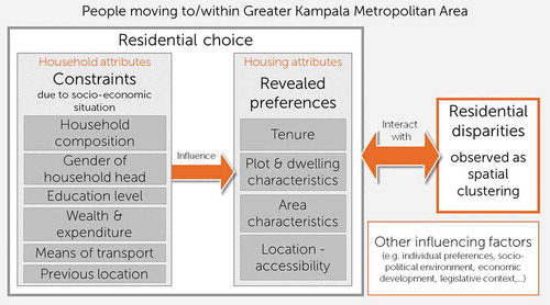
The conceptual framework (Figure 1) thus considers households’ socio-economic situation as the independent variable influencing revealed preferences for certain housing attributes (dependent variable). These together compose residential choice, which interacts with residential disparities identified as spatial clustering at the city level. While other factors such as individual preferences, the socio-political environment, economic development, legislative context, etc. also inform residential mobility and residential choice decisions, these are not included in the analysis.

Figure 1. Conceptual framework. Source: Author

Data and methods

Sampling and data collection

This paper uses data collected within the framework of “Spatial Inequality in Times of Urban Transitions: Complex Land Markets in Uganda and Somaliland (SITU-Transitions),” a research project carried out by a consortium composed of the Institute for Housing and Urban Development Studies (IHS), the Development Planning Unit (DPU) of University College London, IPE Tripleline and local partners. While it uses insights from all the research components, it mostly draws on data from the household survey, conducted in May and June 2018, and from the spatial analysis, carried out in 2017 and 2018. Data were collected and analyzed on four cities, but in this article, the focus is on Kampala.

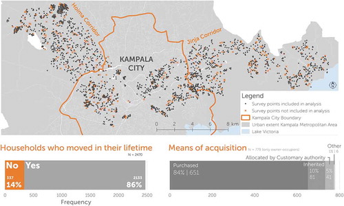
The household survey was conducted along a cross section of Kampala’s urban area, which will be referred to as “cross section” in this article. For delimiting the urban area, the research used functional rather than administrative boundaries of the Greater Kampala Metropolitan Area (GKMA) as they were identified in the spatial assessment (SITU-Transitions, 2018). Recognizing the importance of main access roads for residential land markets, the cross section was set using two main transportation corridors: the Hoima corridor (west) and the Jinja corridor (east).

A multi-stage, stratified probability sample design was used for the household survey. The survey was limited to residential areas in the cross section; areas with mixed use (commercial, institutional and some residential) and nonresidential areas (e.g. infrastructure or industrial areas) were left out. Strata were divided according to corridors and housing types. The latter were identified through the morphological study, part of the spatial assessment, in order to understand different types of settlement areas existing in the GKMA (SITU-Transitions, 2018). Four dominant housing types (types A, B, C and D) were identified in the GKMA, based on overall dwelling characteristics, building density, and the spatial layout of an area. Type A areas are characterized by a regular road grid with large and regularly shaped plots. Type B has a mix of regular and irregular plots with identifiable roads. In Type C areas roads are still identifiable but plots are more irregular and density is higher than in type B areas. Finally, type D has mainly narrow roads and pedestrian paths and irregular small plots with high building density. For a more detailed description of the housing types, see Appendix 1. Sample sizes for individual strata were designed to allow for a 5% degree of error at the 95% confidence level, based on the estimated population of the strata from the spatial assessment. In total, 2,470 usable surveys were included in the database.

In this paper, residential preferences are studied based on households’ choices regarding their current housing and location characteristics. Therefore, households who never moved (337 or 14% of the sample), those who did not choose their location as they obtained access through inheritance or allocation by customary authorities (38; 1.5 percent) or those who did not indicate how they bought or rented their home (37, 1.5 percent) were omitted from the analysis. Analysis for this paper is thus based on 2,058 surveys (see Figure 2).

Figure 2. Household survey points included in the analysis. Source: Author, based on SITU-Transitions research data

Variables and indicators

In the operationalization of this research, the constraints are considered from a household perspective and are therefore linked to the household’s socio-economic characteristics and the information that households had available. A first indicator of the household’s socio-economic characteristics is household composition and is split into six categories: single person household; two adults; one adult with (a) child(ren); two adults with (a) child(ren); a group of more than two adults but no children; and other household composition with (a) child(ren). Age was not differentiated beyond the child/adult distinction, yet this categorization could provide a basic indication of the lifecycle stage the household is in, though further analysis would be needed to confirm. Second, the gender of the household head is taken into account as female-headed households are often considered to be in a more vulnerable situation. A third indicator, education level, takes the highest attained education level of anyone in the household into consideration.

A series of indicators for estimating the household’s economic situation is also included: self-reported wealth is the respondent’s answer to the question “Imagine six steps, where on the bottom, the first step, stand the people, that have the least and on the highest step, the sixth, stand the people that are best off. On which step do you think your household stands today?,” which is reduced to two categories: those who feel they are in the bottom three steps and those who feel in the top three steps. Thus, self-reported wealth will be considered as an actual indicator of wealth. Food expenditures per person per month and water expenditures per person per month are calculated based on the respondent’s reported food and water expenditures for the household per month, divided by the number of household members, where children (under the age of 15) are counted as half. Regarding means of transportation, if the respondent answered that any member of the household used a private car as their main mode of transportation, the indicator private car is marked as “yes.” Lastly, it was assumed that households who moved from further away had less access to information regarding their future location. For the indicator “previous location,” households are divided into three groups: those moving within the same neighborhood, those moving between neighborhoods in the GKMA, and those moving into the area. Four further indicators, i.e. dependency ratio, income level, self-reported expenditures versus income ratio, and electricity expenditures per person per month are omitted to avoid multicollinearity.

Housing attributes of the revealed preferences are operationalized using four main categories:

• Tenure: divided into own and rent. Householders living as caretakers or other are left out in this analysis.

• Plot and dwelling characteristics: dwelling type, dwelling materials, dwelling size and plot conditions and amenities upon moving. For dwelling size, an absolute measure of the number of bedrooms and a relative measure of crowding, calculated as the number of people divided by the number of rooms, are included. Regarding information about the plot conditions, it is important to assess the conditions upon moving as these are the conditions that influenced the household’s decision. The indicator plot condition therefore signifies whether there was a built structure already or if the plot had been vacant when the household moved. The number of amenities is a count of how many of the following amenities were present upon accessing the property: a fence, water connection, electricity, and sanitation.

• Area characteristics reveal information about the conditions of the surrounding area beyond the plot. This indicator is the residential typology, a categorization according to the predominant housing type of the area as evaluated by the spatial assessment (SITU-Transitions, 2018), as described above.

• The residence’s location in relation to other relevant locations for the household is an important consideration. The following indicators are used: Euclidean distance to the city center with the location of the Kampala City Council chosen as the central point; the distance to the closest main road as a measure of accessibility; travel distance to the main location (i.e. the location most traveled to, e.g. work, education, shopping, etc.) of the household head; the average distance to the main location of all household members; the travel time to the main location of the household head and all household members. Lastly, there is a dummy indicator whether the respondent indicated if relatives are living nearby. Other indicators, such as proximity to schools or public services are omitted as either they did not have substantial variation (e.g. when overall distances are quite uniformly short, as is the case with primary schools) or the completeness of the information could not be ensured, which would distort the distance calculation.

Data analysis

Logistic regression analysis is employed to predict revealed preferences based on household characteristics. The type of regression depends on the dependent variable: for dependent indicators that have only two options (tenure, plot condition, relatives living nearby), a binary logistic regression is used; for other categorical indicators (dwelling type, dwelling materials, residential typology, household head and average distance and travel time to main location), the analysis is conducted using a multinomial logistic regression. In the case of ordinal indicators (distance to the main road, travel distance household head, travel time household head), ordinal regression is utilized; for continuous dependent indicators (crowding, distance to city center, average travel distance for all household members and average travel time for all household members), ordinary least squares (OLS) regression is employed; while the distribution of the indicators “number of bedrooms” and “number of amenities” follows a Poisson distribution, therefore a Poisson regression is chosen. For categorical indicators, both in the dependent and the independent variables, the first category is used as the reference.

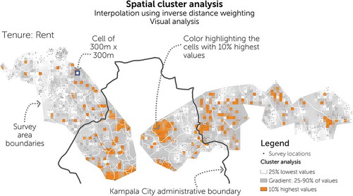
When analyzing residential disparities, the same indicators as above are used, but analyzed with regard to their spatial distribution. Since the distribution of the sample within the geographical sampling area is not regular, a way to disregard the clustering of the sampling itself has to be found. Therefore, although there are several drawbacks to this method, interpolation using inverse distance weighting is used to estimate missing values at a grid of blocks of 300 by 300 meters inside the geographical sample area (roughly described as a convex hull around the outer limit of all the observations and then optically reduced for larger areas without any observations). In order to interpret the data, any indicator has to be transformed in dummy indicators and then analyzed separately. The interpolation thus indicates the estimated ratio of absence/presence for each dummy or the minimum/maximum ratio for continuous variables. In the visualization, the lowest 25% of the values are represented in white; values between 25 and 90% are indicated using a gray gradient, while the highest 10% of the values – the cutoff point set as an indicator of clustering – are marked in color (see example in Figure 3). As minimum and maximum values between the indicators differ, the degree of clustering cannot be compared between the different indicators, only within each indicator as an indication of spatial autocorrelation.

Figure 3. Spatial cluster analysis: example for rental accommodation. Source: Author, based on SITU-Transitions research data

Results

Descriptive statistics

Descriptive statistics are presented in Appendix 2. A typical household in the cross section is male-headed (72% of all surveyed households), composed of three members, of which one is a child. At least one member has finished secondary education (74% of all surveyed households) and they spend around 75 USD per month on food and water, which is on average about a quarter of their total expenditures. They have probably moved to their current location from another neighborhood in the GKMA (39%), do not travel by private car (88%) and perceive themselves to be on the lower half of the wealth spectrum (79%).

In the sample, a typical household rents (61%) a 1-bedroom (34%) tenement style (42%) residential unit built with permanent materials (91%) which, when they moved, had sanitation (70%) and electricity (63%) but not a fence (17%) or a water connection (41%). There is a statistically significant, though weak correlation (r = 0.345, p = <0.001) between the number of people in the household and the number of rooms; on average, there are two people per room. In total, 19% of respondents obtained access to a vacant plot: these are almost exclusively owner occupiers; 99.8 percent of those renting obtained access to a plot with a dwelling on it, whereas for owner occupiers this is only 29%.

A typical household in the cross section lives in a type B (31%) or type C (31%) residential area, characterized by an irregular street layout with identifiable roads and small, irregular plots. They live between 1 and 2 km from the closest main road (40%) and the average distance to the city center is 9.8 km, though these data are in large part determined by the sample location choice. Their daily commute takes about half an hour each way. Only 11% of all respondents indicated that one of the reasons that they chose their location is that they had relatives living nearby.

Regression analysis

The regression analysis analyzes the influence of household attributes on each of the revealed housing preferences. A regression is done for each housing attribute separately. An overview table with the results can be found in Appendix 3.

When comparing preferences for owning or renting, it can be observed that, holding all other indicators constant, singles are much more likely to be renting than any other household composition, although the difference is not statistically significant for those households composed of two adults. Households who consider themselves wealthier are 2.5 times more likely to own; those who indicate that a family member travels by car are almost 5 times more likely to own than those who do not. Altogether, this seems to indicate that owner occupiers tend to be wealthier and perhaps also later in the life cycle than those who rent.

Analyzing the multinomial regression for dwelling type, using detached single family home as the reference category, it is remarkable that (holding all other indicators constant) single parent households are 2.19 times more likely than singles to live in a semi-detached house and 2.66 times more likely to live in a tenement building. Couples and families with children are also more likely to live in tenements, with a factor of 3.21 and 2.23, respectively. Those who indicated being on the bottom half of the wealth distribution are 60% more likely to live in tenement buildings. Having a private car as means of transportation drastically decreases the likelihood to live in semi-detached houses as well as in tenement buildings, with factors 0.27 and 0.08, respectively. Higher levels of education increase the likelihood to live in a semi-detached house with a factor 1.83 for secondary and 1.91 for tertiary education; while those with tertiary education are even 5.4 times more likely to live in an apartment building compared to those with primary education only. In general, the model does not predict well who lives in apartment buildings, as few indicators are statistically significant. This could be linked to the small number of people (n = 73) living in apartment buildings, perhaps in combination with a high variance in the socio-economic situation of inhabitants living in this dwelling type.

The multinomial regression for dwelling materials compares residential units built with semi-permanent and traditional materials to the reference category of permanent materials. The only indicator that shows significance with regard to traditional materials is education: holding all other indicators constant, those with secondary education are twice as likely to live in a dwelling built with permanent materials as those where the highest attained level of any member in the household is primary education; if anyone finished tertiary education, the likelihood is even 11 times. Odds ratios for female-headed households to live in a dwelling built with semi-permanent materials are 2.42 in comparison to male-headed households. Food and water expenditures are also a statistically significant indicator for living in a building of semi-permanent dwelling materials, though the differences are not as pronounced: a dollar increase in per month expenditures on food and on water results in a 0.98 and 0.81 odds ratio for food and water, respectively. Phrased differently, people who live in dwellings built with semi-permanent materials spend less on food and water than those who live in buildings of permanent materials. Interestingly, this does not hold up for those living in structures built with temporary or traditional materials, as shown in the lack of statistically significant indicators in the model. However, as the sample sizes of those living in structures of semi-permanent (n = 128) and traditional materials (n = 49) are small, caution must be exercised regarding its interpretation.

Comparing the influence of socio-economic characteristics on the number of bedrooms in the residential unit, odds ratios for couples and single parent households are similar to those of singles, holding all other indicators constant. However, for couples with children, groups of adults and other households with children, the odds of a one unit increase in the number of bedrooms in comparison to singles are 32; 68; and 78%, respectively. While the increase by itself is logical as any household composition is larger compared to the reference category “singles,” these percentages are below 100%, i.e. the increase is less than a room per additional person. It is expected to see the same trend again in the model for crowding (see below). Furthermore, odds ratios are also statistically significant and positive for education level, traveling by car, and wealth; for each indicator the percentage of change is between 13 and 46% for an additional person.

As expected from the results of the Poisson regression for the number of bedrooms, the results for the linear regression for crowding have a statistically significant and positive standardized beta coefficient for each household composition in comparison to the single reference. This coefficient ranges from +0.17 for a unit increase in crowding (i.e. a doubling of number of persons per room) for couples, to +0.52 for couples with children. Higher education on the other hand leads to less crowding, with a coefficient of up to −0.15 for households with tertiary education. Further, as can be expected, crowding also happens more in less wealthy households (β = −0.08) and in households who spend less on food (β = −0.09) and on water (β = −0.05). While these differences are small, they are statistically significant (p < 0.001).

The binary logistic model for predicting preferences regarding accessing a vacant plot or one with a built structure is not very strong: including the indicators only improves the constant-only model from 80 to 82%. Noticeable is that various household compositions (two adults with children; groups of more than two adults and other households with children), apart from couples and single parents, are more likely than singles to access a vacant plot. The same is true for male-headed households in comparison with female-headed households: holding all other indicators constant, they are 56% more likely to access vacant land. Furthermore, wealthier households and those traveling by car also demonstrate a preference for vacant land. Interestingly, this is the first model where previous location is a statistically significant indicator, though only regarding people moving from within the GKMA as compared to those moving within the same neighborhood: they are 36% less likely to obtain access to vacant land. For predicting the number of amenities (as a count of the following amenities: fence, sanitation, water connection, electricity), having a family member with tertiary education (odds ratio (OR) +30%) and someone traveling by private car (OR – 24%) are the best predictors.

Regarding the multinomial logistic regression for residential typology, the consistently highly statistically significant indicator is “traveling by car”: in comparison to type A, and holding all other indicators constant, responding households are 63% less likely to travel by car in type B, 84% less likely in type C and 94% less likely in type D. Type A, as analyzed in the spatial assessment, is the high-end residential market with large plots, therefore it is not surprising that households choosing these areas are car owners. On the other hand, neither self-reported wealth nor food and water expenditures show statistically significant differences in the odds ratios, apart from a marginal difference for food expenditures in type C. Furthermore, couples and families with children (apart from single adult families) are up to 3.4 times more likely than singles to live in type B, C or D in comparison to type A. If a household prior to moving lived in the GKMA but in a different neighborhood, they were 45% less likely to move to a type D location than those who moved within the neighborhood. This could indicate that residential mobility happening in type D is mainly within the neighborhood.

Interestingly, differences in households’ socio-economic situation only explain 2 percent of the variation in distance to the city center. The most statistically significant indicator is water expenditures, which in this case might be more an indication of location than a predictor. Similarly, in the results for the ordinal regression regarding distance to the main road, only the coefficients for wealth and household head gender are statistically significant. Preferences regarding distance to the city center and distance to the main road, therefore, seem hardly influenced by a household’s socio-economic situation or are too heterogeneous to observe.

The ordinal regressions for travel time and for travel distance to the main location of the household head show very similar results. Household composition is a significant predictor: household heads with children are 63% more likely to travel longer and between 48% and 60% more likely to travel further than singles. Female-headed households seem to prefer to live closer to their main location, both measured in travel time and distance. Household heads where at least one family member travels by car on average travel further and longer than those who do not travel by car. When taking averages of all household members, household composition seems to matter less. Responding households in which a member has completed tertiary education tend to choose a location where on average they have to travel further. The same is true for households where a member travels by car: on average, their distance is a coefficient 0.71 further and even 4.9 times longer.

The overall model of the household’s socio-economic situation does not increase the predictability of moving close to relatives or friends, even though individual predictors such as household composition indicate a statistically significant relationship. Especially households without children are more likely to prefer to move close to relatives or friends, as do female-headed households. Being wealthy on the other hand reduces the preference for (or dependence on?) living close to relatives/friends.

In conclusion, various socio-economic indicators are statistically significant predictors for most housing attributes, though only to a limited extent for the locational attributes of distance to the city center, distance to the main road and moving close to family or friends. There is a difference among socio-economic indicators that are statistically significant, depending on the housing attribute.

Geographical cluster analysis

The geographical cluster analysis is carried out to reveal if and where spatial clusters of specific attributes, both of the household attributes (shown in appendices 4 and 5). Overall, household attributes seem to be quite dispersed, with only an occasional remarkable cluster. Household composition, apart from the singles cluster around Makerere University (most probably the student population), is divided rather evenly, although higher concentrations of households with children seem to be largely outside the administrative area of Kampala City. Distinguishable clustering can be seen in the travel by private car, which bears resemblances to the self-reported wealth. Evaluating the three levels of education, there is a centralizing trend with increasing levels of education. Clusters of high food and water expenditures seem to occur most in the eastward Jinja corridor, mostly within the administrative areas of Kampala City but also somehow spilling over to neighboring Mukono. People’s previous location does not seem to result in any specific spatial clustering.

Clearer indications of spatial autocorrelation are revealed when analyzing the auto-clustering of each housing attribute. Rental accommodation seems to be located much more in the central areas of Kampala; while clusters of high owner occupancy are mostly situated in the outermost edges of the corridors in both directions, though perhaps more pronounced in the Hoima corridor to the west. There seem to be clear pockets of buildings constructed with traditional materials; different but also clustered areas of buildings constructed with semi-permanent materials, while permanent materials are prevalent in almost any area of the city, even if stronger outside the administrative boundaries of Kampala City. With regard to dwelling type, the single most obvious cluster is that of apartment buildings, centrally located in Kampala. However, closer inspection of the other building types also reveals a stronger presence of standalone housing outside the boundaries of Kampala City on the Hoima corridor as compared to the same corridor within Kampala City limits (Rubaga Division).

Unsurprisingly, the clustering of houses with many bedrooms follows a similar pattern of clustering as the wider spaced type A areas, self-reported wealth and traveling by private car. Also, as could be expected, those who accessed a plot with dwelling are closer to the city center. Houses seem to have more amenities in the Jinja corridor as compared to the Hoima corridor.

Since residential typology was identified through a spatial morphological analysis, it naturally displays clustering. Considering the hierarchical nature of the status attached to each type (from highest status to type A to lowest to type D), understanding the main cluster locations for each housing type could help to understand their interconnections with other housing attributes or even household attributes. Thus, type A is most prevalent in central Kampala and in the most outward developments in the Hoima Corridor; type B is observed mostly outside Kampala City boundaries. The same is true for type C, with a very pronounced pocket just outside the Kampala City boundary to the west and smaller pockets in Mukono in the east; and type D almost exclusively occurs within Kampala City boundaries.

Analyzing the spatial distribution of travel distance and time for the household head and an average for each household member yields very similar patterns. Households spending the longest commuting time and traveling furthest are mostly those who live in the Nansana area (just outside the Kampala City border on the Hoima corridor) and those who live at the far end of the Jinja corridor. Lastly, the spatial distribution of households indicating they moved to their location in order to be close to relatives or friends is evenly spread out. In conclusion, while household attributes seem to be rather dispersed over the study area, considerable spatial autocorrelation can be observed in the housing attributes.

Discussion

The intention of this article was to gain a better understanding of the influence of households’ socio-economic situation on residential preferences and how this interacts with the existing morphology of the city so as to obtain insights regarding spatial inequality. The former was done through a regression analysis for each housing attribute. Spatial autocorrelation of each indicator (both household and housing attributes) was tested by conducting a spatial cluster analysis. Below, the three hypotheses that form the basis of this research are discussed before arriving at conclusions about the main research question.

Hypothesis 1: Households’ residential choice is informed by their joint preferences but limited by their socio-economic situation

There are various socio-economic characteristics that prove to be valid predictors of specific preferences, such as tenure choice, size of the house (both absolute size through number of bedrooms and relative size through the crowding indicator), number of amenities, residential typology, and travel time and distance. Significant indicators were mostly household composition, traveling by private car, level of education, and in some cases gender of the household head, food or water expenditures and self-reported wealth. When significant, they mostly predicted in line with what has been found in literature (e.g. Clark et al., 2014; Kim et al., 2015; Schirmer et al., 2014): for example, singles’ preference for renting; the higher likelihood to live in a detached residence for households where a family member travels by private car; households with higher education level who tend to have a residence with more amenities; and wealthier households’ preference for more bedrooms; etc.

Traveling by personal car often proved to be a better predictor of housing options than the self-reported wealth indicator. Only in 12% of the responding households, as car travel is uncommon, there is a family member who travels by private car to their main activity – it might be not just a convenient way of transportation, but also a status symbol and therefore an alternative indicator for a household’s wealth situation, which is consistent with the findings by Diaz Olvera et al. (2013). This relationship between the two indicators is strengthened by the significant, though moderate correlation between them (r = 0.43, p < 0.001) and the visual similarities in the cluster analysis of traveling by car, self-reported wealth, number of bedrooms in the house and type A residential typology, indicative of upper-class neighborhoods.

Assessing the results of the regression analysis, it exposes social inequality in the cross section. On the favored side are certainly those who travel by car and in many respects those who have enjoyed tertiary education. Female-headed households’ alleged vulnerability is only partially confirmed in the regression analyses: they are more likely to live in a house built with semi-permanent dwelling materials, and more likely to live in type C areas. On the other hand, they are more likely to own than male-headed households and also report shorter travel distances and times. Households with children (both single parents and couples), while also more likely to own, might be more vulnerable, therefore negatively affected by the geography of opportunity. They are more likely to live in semi-detached and tenement buildings; experience more crowding; are more likely to live in type B, C and D areas and travel longer to their main location. However, as Spiegel (1986) notes about southern Africa, household compositions can be very fluid, therefore it would be good to confirm these findings using longitudinal research methods.

Hypothesis 2: Housing options are unequally distributed across Kampala

Kampala is a polycentric city, which might be why the regression model for predicting distance to the city center performed so poorly (i.e. only two indicators showed significance, both with only small changes in the Standardized Beta Coefficient). Indeed, socio-economic attributes did a much better job at explaining travel distance and travel time. Relational distance – to work, education or other activities important for the household – is therefore probably a higher priority when looking for a suitable place to live, which is consistent with results obtained by Zondag and Pieters (2005). The similarity between the clustering of the travel distance or time for the household head and the average time and distance of the household seems to indicate that in the residential location decision, all household members are taken into account, not just the household head.

In the spatial analysis, locations where migrants from outside the city settle are dispersed throughout the city, thus not showing any pronounced “spaces of arrival” for migrants from outside the city (e.g. Taubenböck et al., 2018). Previous location, especially for those who most recently moved from outside the GKMA, was also not a significant predictor in any of the regression analyses. This is contrary to the findings of Andreasen et al. (2017), who found that in Arusha (Tanzania), new migrants initially tend to settle in central areas of the city and are often renters. A possible explanation could be that, as various researchers have pointed out (e.g. Mabin, 1990; Potts, 2009), circular migration is a common phenomenon in Africa, so that even if a household most recently moved from outside the GKMA, they might already have access to information and networks in the city. Further research analyzing households’ residential trajectories would be needed to verify the existence and extent of these networks.

Overall, various clusters of housing options can be discerned. These are most pronounced in tenure, dwelling materials, plot condition and residential typology. Relational distance such as commuting time and distance showed moderate patterns, while distance to relatives was not limited to a specific area. Dwelling types are more mixed throughout the study area, with the exception of apartment buildings that are mostly located close to the city center.

Hypothesis 3: Uneven distribution together with residential choice constraints limits households’ equitable access to the city

It is interesting to observe that while housing attributes were often geographically clustered, clustering is much less visually observable in the household characteristics. The cross section seems to be spatially mixed, with all household compositions, education levels, wealth strata represented throughout the city. Even though socio-economic factors influence the choice of housing attributes, and housing attributes themselves are often spatially clustered, this does not result in a similar clustering of household attributes. The spatial distribution of different types of households across the city does not seem to be directly restricted by the clustering of housing attributes.

Yet, this finding does not mean that inequality does not exist, as can be shown in the numerous significant socio-economic predictors for housing characteristics, but it means that these are spatially, at the level of the city, not so easily observable. It is important to emphasize that the geography and unit of observation of the analysis can influence the results. Therefore, more research using different geography levels and level of detail would be needed for comparison.

Conclusions

In response to the overall research question, this research cannot confirm that uneven distribution of housing options together with residential choice constraints limits households’ equitable access to Kampala. It can be concluded that especially household composition, traveling by private car and level of education shape residential preferences in the cross section, most pronounced in the form of tenure choice, size of the house, number of amenities, residential typology, and travel time and distance. Furthermore, discernable patterns can be observed regarding the spatial distribution of housing attributes. However, this is much less obvious, though not completely absent, in the spatial distribution of household characteristics. Therefore, while results show both social inequality (hypothesis 1) and spatial inequality (hypothesis 2), their interrelation (hypothesis 3) is not straightforward. A more detailed analysis combined with qualitative information could clarify in which way social inequality and spatial inequality interrelate in Kampala.

One interpretation could be that location choice is not as restricted by housing attributes as previously assumed. In this case, even though households are restricted in their housing options by their socio-economic situation, the uneven distribution of housing options does not constraint a household’s location choice as such. Spatial inequality would therefore not seem to be exaggerated.

Another possible explanation is that the analysis did not include all relevant attributes. For example, as the survey did not provide reliable information on housing affordability, this aspect was not included in the analysis. With an increasingly commodified housing market, where profit orientations become more important than guaranteeing the right to adequate shelter, this is a pertinent issue to research further.

Furthermore, even if at city level spatial inequality is not observed, changing the geography and the unit of observation could reveal injustices that are not visible at city level. Moreover, it is important to take into consideration how the spatial distribution of housing options and the socioeconomic constraints faced by households in their housing choice changes over time. Therefore, more research at a finer unit of observation and over time is recommended to capture the dynamics.

Lastly, this article focused mainly on the distributive injustice of housing and household attributes, yet as Dikeç (2001) points out, that is only one side of the coin. The other side, the “injustice of spatiality” is about the “produc[tion] and reproduc[tion of] injustice through space” (Dikec, 1793). As this has been a snapshot in time, it would be interesting to see if and how the dynamics are changing and mutually interacting with each other. That way, not only the direction of (in)equal distribution in space would become clearer, but also how patterns of inequality reinforce each other through space.

Acknowledgments

This work was part of the research project “Spatial Inequality in Times of Urban Transitions” supported by the East African Research Fund funded by the UK Department for International Development (DFID) through the Research for Evidence Division (RED) for the benefit of developing countries. This study has been funded by UK aid from the UK government; however the views expressed do not necessarily reflect the UK government’s official policies.

The author wishes to acknowledge the support of the following people: Dorcas Nthoki and Paula Nagler for assistance in the statistical part; Martyn Clark and Colin Marx for feedback; the two anonymous reviewers and the journal editor.

Disclosure statement

No potential conflict of interest was reported by the authors.

Additional information

Funding

This work was supported by the UK Department for International Development (DFID) .

Notes on contributors

Els Keunen

Els Keunen works as urban planning expert at the Institute for Housing and Urban Development Studies (IHS). She has a Master’s degree in Architecture and a Master’s degree in Cultures and Development Studies. She has started a Ph.D. in International Urbanism on the topic of residential mobility in Uganda. Her research interests are residential mobility, spatial inequality, thinking spatially, strategic planning and urban development. Prior to working in academia, Els worked in international cooperation in Uganda and Mozambique for more than six years.

Appendix

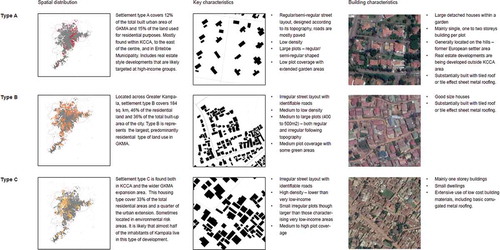
Figure A1. Housing typology descriptions. Source: Spatial Assesment of Kampala, Uganda by.SITU-Transitions (2018)

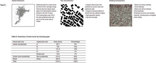
Figure A4. Cluster analysis for household attributes. Source: author, based on SITU-Transitions research data

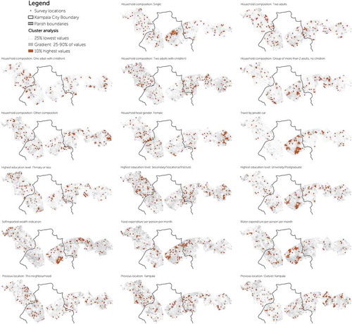
Figure A5. Cluster analysis for housing attributes. Source: author, based on SITU-Transitions research data

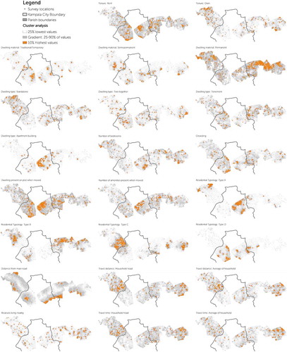
Table B1. Descriptive Statistics

		Obs	Distribution of categorical indicator (Frequency, %)
Variable/indicator name	Type of ind a		0	1	2	3	4	5	6	7	Mean	S.D.	Min	Max	Coding scheme
Household attributes
Socio-economic situation
Household composition	Cat	###		274 13.3%	277 13.5%	150 7.3%	718 34.9%	201 9.8%	437 21.2%			1.65	1	6	1 = Single, 2 = Two adults, 3 = One adult with child(ren), 4 = Two adults with child(ren), 5 = Group of >2 adults, no children, 6 = Other composition
Household head gender	Dum	###		1357 72.0%	527 28.0%							0.45	0	1	0 = Male-headed household, 1 = Female-headed household
Education level	Cat	###		520 25.4%	988 48.2%	540 26.4%						0.72	1	3	1 = Primary or less; 2 = Secondary/Vocational/Institute; 3 = University/Postgraduate
Self-reported wealth indication	Dum	###		1608 78.1%	450 21.9%							0.32	0	1	0 = no, 1 = yes
Food expenditure pp/m	Cont	###									####	####	0.2	75
Water expenditure pp/m	Cont	###									1.72	1.73	0	7
Private car	Dum	###		1805 88.1%	243 11.9%							0.32	0	1	0 = no, 1 = yes
Available information
Previous location	Cat	###		640 31.1%	793 38.5%	625 30.4%						0.78	1	3	1 = This neigbourhood, 2 = Within Kampala, 3 = Outside Kampala
Housing attributes
Tenure	Dum	###		505 28.7%	1254 71.3%							0.45	1	2	0 = Own, 1 = Rent
Plot & dwelling characteristics
Dwelling type	Cat	###		798 38.8%	322 15.6%	865 42.0%	73 3.5%					0.97	1	4	1 = Detached single family residential (standalone), 2 = Semi-Detached multi-family residential (two together), 3 = Horizontally attached multi-family unit (tenement), 4 = Apartment building
Dwelling material	Cat	###		1887 91.4%	128 6.2%	49 2.4%						0.38	1	3	1 = Permanent, 2 = Semi-permanent, 3 = Traditional/Temporary
Dwelling size
Number of bedrooms	Cou	###	11 0.5%	701 34.1%	532 28.9%	268 13.0%	161 7.8%	155 7.5%	114 5.5%	116 5.6%		1.83	0	7	7 = 7 or more
Crowding (No. of people/No. of rooms)	Cont	###									1.91	1.36	0	10
Plot conditions & amenities upon moving
Plot condition	Dum	###		392 19.3%	1644 80.7%							0.39	0	1	0 = Vacant, 1 = With development
No. of amenities	Cou	###	384 19.3%	286 14.4%	662 33.2%	464 23.3%	197 9.9%				1.90	1.24	0	4
Area characteristics
Residential typology	Cat	###		502 24.4%	637 31.0%	631 30.7%	288 14.0%					1.00	1	4	1 = Type A, 2 = Type B, 3 = Type C, 4 = Type D
Proximity
Distance to city center (m)	Cont	###									9775	5110	711	####
Distance to main road	Ord	###		105 5.1%	168 8.2%	228 11.1%	394 19.1%	820 39.8%	343 16.7%			1.37	1	6	1 = <100 m, 2 = 100–250 m, 3 = 250–500 m, 4 = 500–1000 m, 5 = 1000–2000 m, 6 = >2000 m
Distance to main location of household head	Ord	###		281 15.9%	787 44.5%	460 26.0%	240 13.6%					0.91	1	4	1 = Less than 1 km, 2 = 1 to 3 km, 3 = 4 to 8 km, 4 = More than 8 km
Average distance to main location of household members (in km)	Cont	###									2.86	2.05	0.5	9	Calculated as average distance for each household member using the middle of each category/number of household members
Travel time to main location of household head	Ord	###		193 11.0%	748 42.5%	639 36.3%	132 7.5%	50 2.8%				0.89	1	5	1 = Less than 10 minutes, 2 = 10 minutes – 30 minutes, 3 = 31 minutes – 1 hour, 4 = More than 1 hour – 2 hours, 5 = More than 2 hours
Average travel time to main location of household members (in min)	Cont	###									29.7	20.1	5	150	Calculated as average travel time for each household member using the middle of each category/number of household members
Relatives living nearby	Dum	###		1773 89.0%	220 11.0%							0.31	0	1	0 = no, 1 = yes

aType of indicator: Cat = categorical; Cont = Continuous; Cou = Count; Dum = Dummy; Ord = Ordinal

Table B2. Regression tables

	Tenure		Dwelling type (ref: standalone)							Dwelling material (ref: permanent)					Bedrooms		Crowding
			Likelihood Ratio Tests	Two together (semi-detached)		Tenement (horizontally attached)		Apartment building			Semi-permanent		Traditional/temporary
	Binary logistic		Multinomial logistic							Likelihood Ratio Tests	Multinomial logistic				Poisson		OLS
	Exp(B)	S.E.	Sig	Exp(B)	S.E.	Exp(B)	S.E.	Exp(B)	S.E.	Sig	Exp(B)	S.E.	Exp(B)	S.E.	Exp(B)	S.E.	Standardized Beta	t
Household composition (ref: single)	***		***
Two adults	0.505	0.449		1.490	0.305	3.214***	0.305	2.018	0.663		0.901	0.386	0.300	0.685	1.092	0.072	0.173***	0.112
One adult with child(ren)	0.377*	0.479		2.191*	0.380	2.661***	0.380	5.165	0.902		0.724	0.416	0.528	0.771	1.108	0.091	0.200***	0.140
Two adults with child(ren)	0.227***	0.410		1.471	0.250	2.228***	0.250	1.209	0.618		0.748	0.329	0.434	0.457	1.320***	0.062	0.518***	0.097
Group of >2 adults, no children	0.235**	0.446		0.932	0.327	1.261	0.327	0.683	0.708		1.225	0.427	1.143	0.596	1.684***	0.071	0.219***	0.127
Other composition with children	0.084***	0.420		0.800	0.282	1.144	0.282	0.864	0.657		0.732	0.368	0.355	0.598	1.781***	0.066	0.509***	0.109
Household head	0.713*	0.151	*	1.120	0.178	1.308	0.178	0.469	0.460	***	2.424***	0.216	0.672	0.457	0.995	0.036	0.038	0.067
Education (ref: primary or less)			**							*
Secondary/Vocational/Institute	0.743	0.173		1.828**	0.198	0.945	0.198	2.315	0.659		0.782	0.215	0.484*	0.343	1.133**	0.043	−0.148***	0.069
University/postgraduate	0.986	0.213		1.910**	0.242	0.915	0.242	5.375*	0.674		0.383*	0.373	0.090*	1.043	1.373***	0.049	−0.263***	0.088
Self-reported wealth situation	0.400***	0.161	*	1.048	0.190	0.578***	0.190	1.194	0.363	***	0.394*	0.411	0.207	1.024	1.199***	0.038	−0.077***	0.076
Food expenditure pppm (USD)	1.007	0.005	**	1.000	0.005	1.013**	0.005	1.018*	0.009	*	0.978**	0.008	0.980	0.012	1.001	0.001	−0.090***	0.002
Water expenditure pppm (USD)	1.141**	0.046	**	1.125*	0.048	1.119**	0.048	1.182*	0.084	*	0.812**	0.079	0.847	0.131	1.017	0.009	−0.053*	0.018
A family member travels by personal car	0.184***	0.224	***	0.274***	0.279	0.080***	0.279	1.266	0.404		0.486	0.760		0.000	1.459***	0.046	−0.161***	0.104
Previous location (ref: this neighborhood)
Within Kampala	0.708*	0.150		1.039	0.172	0.939	0.172	2.004	0.434		0.847	0.237	0.768	0.404	1.000	0.036	−0.017	0.065
Outside Kampala	0.842	0.168		0.982	0.189	0.963	0.189	2.208	0.458		1.079	0.240	0.916	0.405	1.020	0.039	−0.006	0.071
Constant/Intercept	19.781***	0.453	***	*	0.324	*	0.324	***	0.885	***	***	0.401	*	0.580	1.341***	0.075	***	0.121
N	1612		1820							1816					1820		1814
	Plot condition		Amenities		Residential typology (ref: Type A)
					Likelihood Ratio Tests	Type B		Type C		Type D
	Binary logistic		Poisson		Multinomial logistic
	Exp(B)	S.E.	Exp(B)	S.E.	Sig	Exp(B)	S.E.	Exp(B)	S.E.	Exp(B)	S.E.
Household composition (ref: single)	***				*
Two adults	0.833	0.413	0.919	0.068		1.850*	0.269	1.538	0.266	2.386**	0.329
One adult with child(ren)	0.698	0.458	0.944	0.088		1.414	0.368	1.633	0.344	1.917	0.42
Two adults with child(ren)	0.311***	0.348	0.891	0.059		2.023**	0.233	1.935**	0.227	2.373**	0.291
Group of >2 adults, no children	0.286**	0.387	0.866	0.08		1.664	0.292	0.999	0.309	1.961	0.382
Other composition with children	0.130***	0.356	0.720***	0.07		2.569***	0.268	2.215**	0.266	3.406***	0.334
Household head	0.642**	0.152	0.96	0.044		1.151	0.175	1.531*	0.173	1.343	0.208
Education (ref: primary or less)
Secondary/Vocational/Institute	0.767	0.181	1.06	0.045		1.293	0.178	1.306	0.175	0.908	0.201
University/postgraduate	0.905	0.22	1.303***	0.055		1.356	0.222	1.272	0.222	0.734	0.269
Self-reported wealth situation	0.549***	0.162	0.94	0.049		0.856	0.18	0.829	0.188	0.648	0.248
Food expenditure pppm (USD)	0.999	0.005	1.003**	0.001		0.997	0.004	0.989*	0.005	0.995	0.006
Water expenditure pppm (USD)	1.212***	0.048	1.025*	0.011		0.942	0.044	1.039	0.044	1.045	0.054
A family member travels by personal car	0.320***	0.21	0.807**	0.069	***	0.369***	0.223	0.161***	0.266	0.055***	0.55
Previous location (ref: this neighborhood)	*
Within Kampala	0.733*	0.155	0.95	0.042		0.801	0.167	0.758	0.168	0.554**	0.202
Outside Kampala	1.043	0.176	0.984	0.045		0.797	0.181	0.765	0.182	0.661	0.214
Constant/Intercept	21.475***	0.394	1.815***	0.076			0.294		0.29		0.362
N	1804		1767		1820
	Distance to City Center		Distance to main road		Travel distance HHH		Average travel distance all household members		Travel time HHH		Average travel time all household members		Relatives nearby
	OLS		Ordinal		Ordinal		OLS		Ordinal		OLS		Binary logistic
	Standardized Beta	t	Estimate	S.E.	Estimate	S.E.	Standardized Beta	t	Estimate	S.E.	Standardized Beta	t	Exp(B)	S.E.
Household composition (ref: single)													**
Two adults	−0.017	485.991	−0.143	0.175	0.26	0.188	−0.024	0.194	0.228	0.189	−0.026	1.96	1.986*	0.334
One adult with child(ren)	0.015	611.877	−0.206	0.219	0.479*	0.239	−0.079**	0.244	0.628**	0.24	−0.055	2.454	0.868	0.434
Two adults with child(ren)	0.073	421.573	−0.155	0.152	0.600***	0.164	−0.086*	0.17	0.627***	0.165	−0.043	1.713	1.201	0.315
Group of >2 adults, no children	−0.014	550.944	−0.282	0.198	0.148	0.213	−0.010	0.22	0.312	0.215	0.007	2.212	2.751**	0.358
Other composition with children	0.054	474.913	−0.301	0.171	0.650***	0.185	−0.065	0.191	0.746***	0.186	0.018	1.922	1.85	0.335
Household head	−0.016	292.299	−0.217*	0.105	−0.634***	0.113	−0.011	0.115	−0.550***	0.114	0.043	1.16	1.664**	0.174
Education (ref: primary or less)
Secondary/Vocational/Institute	0.057	301.408	0.032	0.108	0.067	0.116	0.063*	0.118	0.071	0.117	0.031	1.193	1.169	0.206
University/postgraduate	0.017	384.265	−0.220	0.138	0.331*	0.146	0.122***	0.151	0.357*	0.147	0.068*	1.519	1.452	0.249
Self-reported wealth situation	0.053*	332.689	0.366**	0.12	0.235	0.126	0.043	0.13	0.387**	0.128	0.062*	1.31	0.634*	0.231
Food expenditure pppm (USD)	0.006	7.942	−0.006*	0.003	0.002	0.003	0.046	0.003	0.002	0.003	0.031	0.031	1.003	0.005
Water expenditure pppm (USD)	−0.120***	77.919	−0.012	0.028	0.039	0.03	0.038	0.031	0.043	0.031	0.01	0.309	0.99	0.051
A family member travels by personal car	−0.028	451.809	0.008	0.162	0.771***	0.169	0.115***	0.177	0.528**	0.172	0.079**	1.785	0.949	0.294
Previous location (ref: this neighborhood)													*
Within Kampala	0.002	284.724	0.069	0.102	−0.093	0.108	−0.012	0.111	−0.009	0.109	0.007	1.122	0.592**	0.189
Outside Kampala	0.05	308.881	0.001	0.111	−0.218	0.119	−0.032	0.121	−0.024	0.12	0.031	1.224	0.876	0.19
Constant/Intercept	***	526.885					***	0.211			***	2.131	0.074***	0.377
N	1820		1820		1707		1780		1703		1781		1767

References

- Acheampong, R. A., & Anokye, P. A. (2013). Understanding households’ residential location choice in Kumasi’s peri-urban settlements and the implications for sustainable urban growth. Research on Humanities and Social Sciences, 3(9), 60–70. https://www.iiste.org/Journals/index.php/RHSS/article/view/6317
- Akampumuza, P., & Matsuda, H. (2017). Weather shocks and urban livelihood strategies: The gender dimension of household vulnerability in the Kumi district of Uganda. The Journal of Development Studies, 53(6), 953–970. https://doi.org/10.1080/00220388.2016.1214723
- Andersen, J. E., Jenkins, P., & Nielsen, M. (2015). Who plans the African city? A case study of Maputo: Part 2–agency in action. International Development Planning Review, 37(4), 423–443. https://doi.org/10.3828/idpr.2015.25
- Andreasen, M. H., Agergaard, J., & Møller-Jensen, L. (2017). Suburbanisation, homeownership aspirations and urban housing: Exploring urban expansion in Dar es Salaam. Urban Studies, 54(10), 2342–2359. https://doi.org/10.1177/0042098016643303
- Angel, S., Parent, J., Civco, D. L., & Blei, A. M. (2011). Making room for a planet of cities. Lincoln Institute of Land Policy. https://www.lincolninst.edu/publications/policy-focus-reports/making-room-planet-cities
- Arku, G., Luginaah, I., Mkandawire, P., Baiden, P., & Asiedu, A. B. (2011). Housing and health in three contrasting neighbourhoods in Accra, Ghana. Social Science & Medicine, 72(11), 1864–1872. https://doi.org/10.1016/j.socscimed.2011.03.023
- Bogdon, A. S., & Can, A. (1997). Indicators of Local Housing Affordability: Comparative and Spatial Approaches. Real Estate Economics, 25(1),43-80. doi:10.1111/reec.1997.25.issue-1
- Bruch, E. E., & Mare, R. D. (2012). Methodological issues in the analysis of residential preferences, residential mobility, and neighborhood change. Sociological Methodology, 42(1), 103–154. https://doi.org/10.1177/0081175012444105
- Cassiers, T., & Kesteloot, C. (2012). Socio-spatial inequalities and social cohesion in European cities. Urban Studies, 49(9), 1909–1924. https://doi.org/10.1177/0042098012444888
- Clark, W. A. V., van Ham, M., & Coulter, R. (2014). Spatial mobility and social outcomes. Journal of Housing and the Built Environment, 29(4), 699–727. https://doi.org/10.1007/s10901-013-9375-0
- Coulter, R., & van Ham, M. (2013). Following people through time: An analysis of individual residential mobility biographies. Housing Studies, 28(7), 1037–1055. https://doi.org/10.1080/02673037.2013.783903
- Coulter, R., Van Ham, M., & Findlay, A. M. (2016). Re-thinking residential mobility: Linking lives through time and space. Progress in Human Geography, 40(3), 352–374. https://doi.org/10.1177/0309132515575417
- Diaz Olvera, L., Plat, D., & Pochet, P. (2013). The puzzle of mobility and access to the city in Sub-Saharan Africa. Journal of Transport Geography, 32(2013), 56–64. https://doi.org/10.1016/j.jtrangeo.2013.08.009
- Dieleman, F. M. (2001). Modelling residential mobility; a review of trends in research. Journal of Housing and the Built Environment, 16(3–4), 249–265. https://doi.org/10.1023/A:1012515709292
- Dikeç, M. (2001). Justice and the Spatial Imagination. Environment and Planning A: Economy and Space, 33(10), 1785–1805. https://doi.org/10.1068/a3467
- Eliasson, J. (2010). The influence of accessibility on residential location. In F. Pagliara, J. Preston, & D. Simmonds (Eds.), Residential location choice (pp. 137–164). Springer Verlag. https://doi.org/10.1007/978-3-642-12788-5_1
- Goebel, A., Dodson, B., & Hill, T. (2010). Urban advantage or Urban penalty? A case study of female-headed households in a South African city. Health & Place, 16(3), 573–580. https://doi.org/10.1016/j.healthplace.2010.01.002
- Hedman, L., van Ham, M., & Manley, D. (2011). Neighbourhood choice and neighbourhood reproduction. Environment and Planning A: Economy and Space, 43(6), 1381–1399. https://doi.org/10.1068/a43453
- Ioannides, Y. M., & Kan, K. (1996). Structural estimation of residential mobility and housing tenure choice. Journal of Regional Science, 36(3), 335–363. https://doi.org/10.1111/j.1467-9787.1996.tb01107.x
- Kim, H., Woosnam, K. M., Marcouiller, D. W., Aleshinloye, K. D., & Choi, Y. (2015). Residential mobility, urban preference, and human settlement: A South Korean case study. Habitat International, 49(2015), 497–507. https://doi.org/10.1016/j.habitatint.2015.07.003
- Kombe, W. J. (2005). Land use dynamics in peri-urban areas and their implications on the urban growth and form: The case of Dar es Salaam, Tanzania. Habitat International, 29(1), 113–135. https://doi.org/10.1016/S0197-3975(03)00076-6
- Lee, B. H. Y., & Waddell, P. (2010). Residential mobility and location choice: A nested logit model with sampling of alternatives. Transportation, 37(4), 587–601. https://doi.org/10.1007/s11116-010-9270-4
- Mabin, A. (1990). Limits of urban transition models in understanding South African urbanisation. Development Southern Africa, 7(3), 311–322. https://doi.org/10.1080/03768359008439523
- Manley, D., & Van Ham, M. (2012). Neighbourhood effects, housing tenure and individual employment outcomes. In M. van Ham, D. Manley, N. Bailey, L. Simpson & D. Maclennan (Eds.) Neighbourhood effects research: New perspectives (pp. 147-173). Springer. https://doi-org.eur.idm.oclc.org/10.1007/978-94-007-2309-2_1
- Potts, D. (2009). The slowing of sub-Saharan Africa’s urbanization: Evidence and implications for urban livelihoods. Environment and Urbanization, 21(1), 253–259. https://doi.org/10.1177/0956247809103026
- Roseman, C. C. (1971). Migration as a spatial and temporal process. Annals of the Association of American Geographers, 61(3), 589–598. https://doi.org/10.1111/j.1467-8306.1971.tb00809.x
- Rosenbaum, J. E., Reynolds, L., & Deluca, S. (2002). How do places matter? The geography of opportunity, self-efficacy and a look inside the black box of residential mobility. Housing Studies, 17(1), 71–82. https://doi.org/10.1080/02673030120105901
- Sabagh, G. (1969). Some determinants of intrametropolitan residential mobility: Conceptual considerations. Social Forces, 48(1), 88–98. https://doi-org.eur.idm.oclc.org/10.1093/sf/48.1.88
- Schirmer, P. M., Van Eggermond, M. A. B., & Axhausen, K. W. (2014). The role of location in residential location choice models: A review of literature. Journal of Transport and Land Use, 7(2), 3. https://doi.org/10.5198/jtlu.v7i2.740
- Sharkey, P. (2012). Residential mobility and the reproduction of unequal neighborhoods. Cityscape, 14(3), 9–31. www.jstor.org/stable/41958938
- SITU-Transitions. (2018). Spatial assessment of Kampala, Uganda [Research report]. IPE Tripleline.
- SITU-Transitions. (2019). SITU household survey report Uganda [Research report].
- Smith, B., & Olaru, D. (2013). Lifecycle stages and residential location choice in the presence of latent preference heterogeneity. Environment and Planning A: Economy and Space, 45(10), 2495–2514. https://doi.org/10.1068/a45490
- Spiegel, A. D. (1986). The fluidity of household composition in matatiele, Transkei: A methodological problem. African Studies, 45(1), 17–35. https://doi.org/10.1080/00020188608707648
- Taubenböck, H., Kraff, N. J., & Wurm, M. (2018). The morphology of the Arrival City - A global categorization based on literature surveys and remotely sensed data. Applied Geography, 92(2018), 150–167. https://doi.org/10.1016/j.apgeog.2018.02.002
- Uganda Bureau of Statistics (UBOS). (2017). The national population and housing census 2014 – Area specific profile series, Kampala, Uganda (p. 119). Uganda Bureau of Statistics. https://www.ubos.org/publications/constituency-profiles/
- Van Ommeren, J., & Van Leuvensteijn, M. (2005). New evidence of the effect of transaction costs on residential mobility. Journal of Regional Science, 45(4), 681–702. https://doi.org/10.1111/j.0022-4146.2005.00389.x
- Wentzel, M., Viljoen, J., & Kok, P. (2006). Contemporary South African migration patterns and intentions. In P. Kok, D. Gelderblom, J.O. Oucho & J. van Zyl (Eds.) Migration in South and southern Africa: Dynamics and determinants (pp. 171–204). HSRC Press. https://doi.org/10.13140/2.1.4812.8969
- Zondag, B., & Pieters, M. (2005). Influence of accessibility on residential location choice. Transportation Research Record: Journal of the Transportation Research Board, 1902(1), 63–70. https://doi.org/10.3141/1902-08
- Zorlu, A. (2009). Ethnic differences in spatial mobility: The impact of family ties. Population, Space and Place, 15(4), 323–342. https://doi.org/10.1002/psp.560